HAL Id: tel-01289267
https://tel.archives-ouvertes.fr/tel-01289267
Submitted on 16 Mar 2016
HAL is a multi-disciplinary open access
archive for the deposit and dissemination of sci-entific research documents, whether they are pub-lished or not. The documents may come from teaching and research institutions in France or abroad, or from public or private research centers.
L’archive ouverte pluridisciplinaire HAL, est destinée au dépôt et à la diffusion de documents scientifiques de niveau recherche, publiés ou non, émanant des établissements d’enseignement et de recherche français ou étrangers, des laboratoires publics ou privés.
Gabriela Montoya
To cite this version:
Gabriela Montoya. Answering SPARQL Queries using Views. Databases [cs.DB]. Université de Nantes, 2016. English. �tel-01289267�
Thèse de Doctorat
Gabriela M
ONTOYA
Mémoire présenté en vue de l’obtention du
grade de Docteur de l’Université de Nantes
sous le sceau de l’Université Bretagne Loire
École doctorale : Sciences et technologies de l’information, et mathématiques Discipline : Informatique et applications, section CNU 27
Unité de recherche : Laboratoire d’informatique de Nantes-Atlantique (LINA) Soutenue le 11 mars 2016
Answering SPARQL Queries using Views
JURY
Rapporteurs : M. Bernd AMANN, Professeur, Université de Pierre et Marie Curie (Paris 6)
M. Fabien GANDON, Directeur de Recherche, INRIA Sophia Antipolis Examinateurs : M. Philippe LAMARRE, Professeur, INSA Lyon
MmePascale KUNTZ, Professeur, Université de Nantes
MmeMaria-Esther VIDAL, Professeur, Universidad Simón Bolívar
Directeur de thèse : M. Pascal MOLLI, Professeur, Université de Nantes
Acknowledgements
This PhD thesis was funded by the CNRS (Unit UMR6241).
Experiments presented in Chapter 8were carried out using the Grid’5000 testbed, supported by a scientific interest group hosted by Inria and including CNRS, RENATER and several Universities as well as other organizations (see https://www.grid5000.fr).
1
Introduction
1.1
Context
The Semantic Web is an extension of the Web, where information has precise meaning, and machines are able to understand the information and perform sophisticated tasks for the users [12]. In order to achieve the potential of the Semantic Web, the World Wide Web Consortium (W3C) has defined standards [75]: (i) for the representation of information on the Semantic Web, the Resource Description Framework (RDF) [52]; (ii) for querying the Semantic Web, the SPARQL language [66]; and (iii) for defining richer representations that contemplate intrinsic aspects of the reality, it has defined the Web Ontology Language (OWL) [63]. The number of sources has greatly increased in the last years, e.g., from 2011 to 2014 the increase was of 271% [72], and different actors of the society have published semantic data: scientific publications, e.g. the DBLP Bibliography Database1, media,
e.g., the Jamendo music repository2, geography, e.g. the Norwegian geo-divisions3, government, e.g., the UK transport dataset4, life science, e.g., the UniProt dataset5, and social networking, e.g., foaf
1. http://dblp.l3s.de/d2r/, November, 2015. 2. http://dbtune.org/jamendo/sparql/, November, 2015. 3. http://data.lenka.no/sparql, November, 2015. 4. http://openuplabs.tso.co.uk/sparql/gov-transport, November, 2015. 5. http://sparql.uniprot.org/, November, 2015. 5
profiles6.
The Linked Data is a set of best practices for publishing and connecting structured data on the Web [13]. More than one thousand sources with semantic data have been crawled.7 For many
of these sources, there are infrastructures to execute SPARQL queries called SPARQL endpoints.8
These endpoints allow users to explore datasets, and existing federated SPARQL query engines, such as FedX [74], ANAPSID [2] and SPLENDID [32], can use these endpoints to process SPARQL queries that require data from several endpoints to produce answers, i.e., federated queries, without having to move the data.
Some exemplar Semantic Web applications are the Linked Data Search Engines such as Swoogle [25], Sindice [61], and Watson [23]. These engines allow applications to traverse the Semantic Web, and retrieve meaningful and relevant data. Other exemplar Semantic Web application is service match-making [51], where semantic annotations are used in an e-commerce scenario where seekers search advertisers that satisfy a given set of characteristics. Another exemplar Semantic Web application is link prediction [78], where existing links among entities are used to propose new potential links, and focus the expert efforts on testing these potential links. Some other examples of Semantic Web applications are the analysis of governmental reforms [16], and health monitoring in smart houses [67]. The advantages that the Semantic Web and Linked Data have, with respect to Databases and the traditional Web, are the openness and meaningfulness of data. Openness because, as in the Web for documents, any piece of data can be linked to existing data, and links among data can be followed to discover new data. Meaningfulness because, as in Databases for entities, if two pieces of data are linked, their link has a precise meaning, and several types of links are possible to appropriately represent different kinds of relations.
We are interested by two issues in the context of Semantic Web. First, even if there is a large number of Linked Data sources, many sources from the Web [37] cannot be queried in conjunction with Linked Data sources using SPARQL, and this significantly reduces the space of queries that can be answered. Second, the low data availability provided by SPARQL endpoints [81] that prevents Semantic Web applications from relying on these infrastructures.
To address our first issue, integration of Deep Web sources with Linked Data to answer
6. e.g.,http://www.w3.org/People/Berners-Lee/card.rdf, November, 2015.
7. According to the 2014 report about the state of Linking Data Cloud available at http:// linkeddatacatalog.dws.informatik.uni-mannheim.de/state/
SPARQL queries, there are two approaches. In the Data Warehousing approach [77], sources available in the Web can be transformed into RDF data using platforms such as Datalift [71], and their data can be linked with Linked Data sources using frameworks such as Silk [84]. However, this strategy to transform the Web sources into RDF has some limitations: (i) this transformation and linking should be done for all the known sources before executing any query; (ii) each time a source changes, transformation and linking of the whole source needs to be repeated to avoid stale answers. In the Mediators and Wrappers approach [85], mediators can be used to integrate data without having to move it from sources to the clients, therefore up to date data is queried. Among the mediator paradigms, the best suited for dynamic contexts, such as the Web, is the Local-as-View (LAV) paradigm [1]. Nevertheless, LAV traditional techniques used to produce query answers, query
rewritings, may be too expensive in the context of SPARQL queries and numerous sources [56]. We are interested by strategies that are able to produce query answers against a set of LAV views, but without using query rewritings, i.e., strategies that load the data available through these views into an RDF graph, and execute the query against this RDF graph. These strategies do move data from sources to the mediator, but only the data from the selected views and only during query execution. In this thesis, we address this issue, and in particular the following research question:
Research Question 1. In which order should the query relevant views be loaded into a graph, built
during query execution, in order to use this graph to answer the query, and outperform the traditional LAV query rewriting techniques in terms of number of answers produced by time unit?
To answer this research question, we propose the SemLAV approach. SemLAV integrates hetero-geneous data from Linked Data and Deep Web, following the Local-as-View (LAV) paradigm [1] to describe the setup. Relevant views are ranked according to their possible contribution to the answers, and they are loaded into a graph instance, built during query execution, to answer SPARQL queries. We have two contributions that address this first issue. Our first contribution is the formalization of the Maximal Coverage problem (MaxCov), it consists in selecting the k views to load in order to cover the greater number of rewritings. Our second contribution is the SemLAV relevant view selection and ranking algorithm, this algorithm sorts views according to the number of query subgoals that they cover, and ranks first the views that cover more query subgoals. It allows to load sources that may contribute more to the query answer first, and consequently to produce answers as soon as possible. Experimental results suggest that SemLAV outperforms traditional query rewriting
strategies. These contributions have been published in [56].
To address our second issue, the SPARQL endpoints poor availability, several strategies may be used. The Linked Data Fragments (LDF) [81] have been proposed to exploit client resources to relieve server resources and improve data availability. However, as each client has to perform most of the query processing, this strategy decreases the query performance in terms of number of answers produced by time unit, and amount of transferred data from servers to clients. A distributed query processing strategy to improve data availability is to give data consumers a more active role, and use their resources to replicate data, and consequently increase the data availability [45]. However, as Linked Data consumers are autonomous participants, the replication cannot closely follow the techniques used in distributed query processing, and new strategies to select and localize sources are needed. In this thesis, we are interested in improving data availability by using replication, and in particular the use of fragment replication. Replicating fragments leads to concerns about performance of query processing. For instance, if replicated fragments from popular sources are available through many endpoints, how are these endpoints going to be used to execute a federated query? A very simple solution may be to declare all these endpoints as part of the federation used by the federated query engine. However, this simple solution may incur in high execution time because redundant data would be transferred from endpoints to the federated query engine, and the federated query engine would have to execute the query joins. For example, executing a DBpedia query against a federation with one or two copies of DBpedia, leads to an increase of two orders of magnitude in the execution time for federated query engines FedX [74] and ANAPSID [2] as shown in Section 8.1. In order to properly exploit the benefits of replicated fragments, we propose a source selection strategy that is aware of fragment replication, and is able to enhance federated query processing engines. This idea of exposing replicated fragments through Linked Data endpoints is new, and so there are no existing techniques that are able to perform a source selection aware of data replication. Even if techniques to detect data overlapping based on data summaries exist [38, 70], applying them to scenarios with data replication will incur in expensive computations that are unnecessary in a replication scenario.
In this thesis, we address this issue, and want to answer the following research questions:
Research Question 2. Can the knowledge about fragment replication be used to reduce the number
of selected sources by federated query engines while producing the same answers?
of individual triple patterns, produce source selections that lead to transfer less data from endpoints to the federated query engine?
To answer these research questions, we propose the Fedra approach. Fedra selects the sources to be contacted to evaluate each triple pattern in order to produce the query answers, this selection aims to improve the query performance in terms of the number of transferred tuples during query execution.
We have two contributions that address this second issue. Our first contribution is the formal-ization of the Source Selection Problem with Fragment Replication (SSP-FR). Given a federation of SPARQL endpoints that have replicated fragments, and a SPARQL query, it consists in selecting the sources that have to be contacted to retrieve data for each query triple pattern, such that the num-ber of transferred tuples from sources to the federated query engine is reduced, and all the answers obtainable using the federation data are produced. Our second contribution is the Fedra source selection algorithm, this algorithm approximates the SSP-FR problem. It uses query containment and equivalence among the fragment definitions to prune sources that provide redundant data, and an heuristic for set covering [41] to reduce the number of different endpoints used to retrieve data for the triple patterns of a basic graph pattern. State-of-the-art federated query engines, ANAPSID [2] and FedX [74], have been extended with Fedra source selection strategy, and empirical results show
that Fedra enhances the federated query engines, and mostly reduces the number of selected sources and number of transferred tuples. These contributions have been published in [59].
1.2
Outline
This thesis is composed of two parts. Part I presents our contributions to address the issue of
integration of Deep Web sources with Linked Data to answer SPARQL queries, while
Part II presents our contributions to address the issue of the SPARQL endpoints poor
avail-ability. Chapter 2 presents background concepts related to the Semantic Web, and conjunctive
queries, that are used through the thesis. Readers familiar with the Semantic Web technologies and conjunctive queries terminology may want to skip Chapter2. In addition to this background chapter, each part has its own background sections: Section5.1 for Part I and Section 8.1 for Part II.
1.2.1
Part
I: Answering SPARQL queries using Linked Data and Deep
Web sources
— Chapter 3 gives an introduction to the Answering SPARQL queries using Linked Data and
Deep Web sources part.
— Chapter4presents state of the art for querying the Web of Data, Data Integration, and Query Rewriting.
— Chapter 5 defines the MaxCov problem, SemLAV query execution approach, algorithms, and experimental results.
1.2.2
Part
II: Answering SPARQL Queries against Federations with
Replicated Fragments
— Chapter 6 gives an introduction to the Answering SPARQL Queries against Federations with
Replicated Fragments part.
— Chapter 7 presents state of the art for Distributed Databases and Linked Data query process-ing, source selection strategies for federated queries, and strategies to overcome availability limitations in Linked Data.
— Chapter 8 defines the SSP-FR problem, the Fedra source selection algorithm, and some
experimental results.
1.3
Publications list
This work led to the following publications:
1. Gabriela Montoya, Hala Skaf-Molli, Pascal Molli, and Maria-Esther Vidal. Federated SPARQL Queries Processing with Replicated Fragments. In The Semantic Web - ISWC 2015 - 14th
International Semantic Web Conference, pages 36–51, Bethlehem, United States, October 2015
2. Gabriela Montoya, Luis Daniel Ibáñez, Hala Skaf-Molli, Pascal Molli, and Maria-Esther Vidal. SemLAV: Local-As-View Mediation for SPARQL Queries. Transactions on Large-Scale
3. Pauline Folz, Gabriela Montoya, Hala Skaf-Molli, Pascal Molli, and Maria-Esther Vidal. SemLAV: Querying Deep Web and Linked Open Data with SPARQL. In ESWC: Extended Semantic Web
Conference, volume 476 of The Semantic Web: ESWC 2014 Satellite Events, pages 332 – 337,
Anissaras/Hersonissou, Greece, May 2014. This work is a demonstration of the work in [56]. 4. Pauline Folz, Gabriela Montoya, Hala Skaf-Molli, Pascal Molli, and Maria-Esther Vidal.
Par-allel data loading during querying deep web and linked open data with SPARQL. In Thorsten Liebig and Achille Fokoue, editors, Proceedings of the 11th International Workshop on
Scal-able Semantic Web Knowledge Base Systems co-located with 14th International Semantic Web Conference (ISWC 2015), Bethlehem, PA, USA, October 11, 2015., volume 1457 of CEUR Workshop Proceedings, pages 63–74. CEUR-WS.org, 2015. This work proposes an optimization
of [56].
I also collaborated in two other papers that are not detailed in this dissertation:
— Gabriela Montoya, Luis Daniel Ibáñez, Hala Skaf-Molli, Pascal Molli, and Maria-Esther Vidal. Gun: An efficient execution strategy for querying the web of data. In Hendrik Decker, Lenka Lhotská, Sebastian Link, Josef Basl, and A Min Tjoa, editors, DEXA (1), volume 8055 of
Lecture Notes in Computer Science, pages 180–194. Springer, 2013. This work leaded to the
work in [56].
— Maria-Esther Vidal, Simon Castillo, Maribel Acosta, Gabriela Montoya, and Guillermo Palma. On the Selection of SPARQL Endpoints to Efficiently Execute Federated SPARQL Queries.
Transactions on Large-Scale Data- and Knowledge-Centered Systems, 2015. This paper extends
the source selection work done before starting this PhD thesis [60]. And presented this thesis work at the doctoral consortium paper:
— Gabriela Montoya. Answering SPARQL Queries using Views. ISWC-DC 2015 The ISWC 2015
2
Background
In this chapter we present background concepts related to the Semantic Web and conjunctive queries. In the following section, standards used to represent data in the Semantic Web, and query these data are presented.
2.1
Semantic Web
The World Wide Web Consortium (W3C)1 has developed standards to allow machines to
under-stand the semantics behind the data published on the Web, increasing their possible interactions, and enhancing their data processing capabilities. Data enhanced with semantics, Linked Data, rely on Se-mantic Web technologies such as RDF, SPARQL, OWL and SKOS. Data is stored using the common format RDF, queries are posed using the standard language SPARQL, and vocabularies can be built using ontologies (e.g., using OWL). The Resource Description Framework (RDF) [52] is a framework for representing information in the Web. The basic unit of information are RDF triples, henceforth called triples. Each triple consists of a subject, a predicate and an object. The predicate describes the subject with a given characteristic whose value is given by the object. For example, in Listing2.1, a film is described with two characteristics, first, its director, and second its name. Each resource
1. http://www.w3.org, July 2015.
is identified using IRIs, e.g., the director is identified by IRI http://dbpedia.org/resource/ The_Rules_of_the_Game, also the predicates or properties are identified by IRIs, e.g., the film director is identified by the IRI http://dbpedia.org/ontology/director. Objects may be IRIs, e.g., http://dbpedia.org/resource/Jean_Renoir, or literals, e.g., “The Rules of the Game”@en. Literals may be strings, numbers, dates, etc. Strings may be annotated using language tags, e.g., ’@en’ indicates that the string language is English.
Listing 2.1 – Two RDF triples that describe a film
<h t t p : / / d b p e d i a . o r g / r e s o u r c e / The_Rules_of_the_Game>
<h t t p : / / d b p e d i a . o r g / o n t o l o g y / d i r e c t o r > <h t t p : / / d b p e d i a . o r g / r e s o u r c e / J e a n _ R e n o i r > . <h t t p : / / d b p e d i a . o r g / r e s o u r c e / The_Rules_of_the_Game>
<h t t p : / / d b p e d i a . o r g / p r o p e r t y /name> " The R u l e s o f t h e Game" @en .
IRIs in Listing2.1are part of DBpedia vocabularies2. DBpedia resources have IRIs that start with
“http://dbpedia.org/resource/”, this common prefix is called namespace IRI, and it may be associated with a namespace prefix, for “http://dbpedia.org/resource/” we have the namespace prefix “dbr”, and the resource <http://dbpedia.org/resource/Jean_Renoir> may be written as dbr:Jean_Renoir using the namespace prefix. Listing 2.2 shows the same triples of Listing 2.1 using namespace prefixes.
Listing 2.2 – Two RDF triples that describe a film, with prefixes
PREFIX d b r :< h t t p : / / d b p e d i a . o r g / r e s o u r c e /> PREFIX dbo :< h t t p : / / d b p e d i a . o r g / o n t o l o g y /> PREFIX dbp :< h t t p : / / d b p e d i a . o r g / p r o p e r t y />
d b r : The_Rules_of_the_Game dbo : d i r e c t o r d b r : J e a n _ R e n o i r .
d b r : The_Rules_of_the_Game dbp : name " The R u l e s o f t h e Game" @en .
When the prefixes are well-known or clear from the context, their declaration may be omitted. A RDF graph is defined as a set of RDF triples. And a RDF dataset is composed by a set of RDF graphs.
Once data is represented using the RDF framework, it may be queried using the SPARQL lan-guage. For instance, if we want to know who is the director of “The Rules of the Game” film, we may obtain it using the query in Listing 2.3. This query is composed of two triple patterns. Each triple pattern is composed of a subject, a predicate and an object as an RDF triple is, but each of these components may be a variable. For example, the first triple pattern has as subject the variable ?film, and as object the variable ?director. Variables are denoted by strings that start with character
‘?’ or ‘$’, in this thesis we will use variables starting with character ‘?’. The two triple patterns in Listing2.3 compose a basic graph pattern. A basic graph pattern is a group of triple patterns, with no other operator between than ‘.’, this operator represents the conjunction, i.e., both triple patterns should be satisfied, and common variables among the triples represent a join condition of equality.
Listing 2.3 – SPARQL SELECT query that retrieves the director of a film
SELECT ? d i r e c t o r WHERE {
? f i l m dbo : d i r e c t o r ? d i r e c t o r .
? f i l m dbp : name " The R u l e s o f t h e Game" @en }
The answer to a SELECT query, as the one given in Listing2.3, is a set of mappings. A mapping is a pair (variable, value). This set of mappings indicates the values that the variables in the WHERE should be instantiated to in order to obtain triples that belong to queried dataset. For example, the query in Listing 2.3, evaluated against the dataset in Listing 2.1, has as answer { (director, http://dbpedia.org/resource/Jean_Renoir) }.
Listing 2.4 – SPARQL ASK query that checks if there are triples with the director of a given film
ASK {
? f i l m dbo : d i r e c t o r ? d i r e c t o r .
? f i l m dbp : name " The R u l e s o f t h e Game" @en }
Besides SELECT queries, there are three other query types in SPARQL: ASK, CONSTRUCT and DESCRIBE queries. ASK queries have a query pattern, like the one included in the WHERE clause of SELECT queries, and its answer is a boolean value. Its answer is true if and only if there is a set of mappings such that the query triple patterns with their variables instantiated to the values in the set of mappings correspond to triples that belong to the queried dataset. For example, the query given in Listing 2.4, evaluated against the dataset in Listing 2.1, has as answer true.
Listing 2.5 – SPARQL CONSTRUCT query that returns a graph with the directed films
CONSTRUCT {
? d i r e c t o r <h t t p : / / e x a m p l e . o r g / d i r e c t s > ? f i l m } WHERE {
? f i l m dbo : d i r e c t o r ? d i r e c t o r . }
@ p r e f i x n s 0 : <h t t p : / / e x a m p l e . o r g /> .
@ p r e f i x d b r : <h t t p : / / d b p e d i a . o r g / r e s o u r c e /> .
d b r : J e a n _ R e n o i r n s 0 : d i r e c t s d b r : The_Rules_of_the_Game .
Listing 2.7 – SPARQL CONSTRUCT query that returns a graph with the film directors
CONSTRUCT {
? f i l m dbo : d i r e c t o r ? d i r e c t o r } WHERE {
? f i l m dbo : d i r e c t o r ? d i r e c t o r }
Listing 2.8 – SPARQL CONSTRUCT query that returns a graph with the film directors, using abbreviation for CONSTRUCT queries with graph template and pattern that are equal
CONSTRUCT WHERE {
? f i l m dbo : d i r e c t o r ? d i r e c t o r }
Listing 2.9 – Answer to the SPARQL queries in Listings 2.7 and 2.8, evaluated against the dataset in Listing 2.1
@ p r e f i x dbo :< h t t p : / / d b p e d i a . o r g / o n t o l o g y /> . @ p r e f i x d b r : <h t t p : / / d b p e d i a . o r g / r e s o u r c e /> .
d b r : The_Rules_of_the_Game dbo : d i r e c t o r d b r : J e a n _ R e n o i r .
CONSTRUCT queries have a graph template and a graph pattern, the graph pattern as in SELECT queries is introduced after the WHERE keyword. CONSTRUCT queries return a RDF graph. The variables instantiations obtained from the graph pattern are used to instantiate the variables in the graph template, and the ground triples, i.e., triples with only IRIs or literals, obtained from the graph template are combined in a single RDF graph. Listing2.5 presents an example of a CONSTRUCT query with graph template and pattern that are different, its answer is presented in Listing2.6. Notice that the variables used in the graph template are also used in the graph pattern. Listing 2.7 shows an example where the graph template and pattern are equal, in such cases the query may be abbreviated as in Listing 2.8, the answer to this query, evaluated against the dataset in Listing 2.1, is presented in Listing2.9.
Listing 2.10 – SPARQL DESCRIBE query that returns a graph with a film description
Listing 2.11 – SPARQL DESCRIBE query that returns a graph with films and directors description
DESCRIBE ? f i l m ? d i r e c t o r WHERE {
? f i l m dbo : d i r e c t o r ? d i r e c t o r }
Listing 2.12 – Answer to the SPARQL queries in Listings2.10and2.11, evaluated against the dataset in Listing 2.1
@ p r e f i x dbo :< h t t p : / / d b p e d i a . o r g / o n t o l o g y /> . @ p r e f i x dbp :< h t t p : / / d b p e d i a . o r g / p r o p e r t y /> . @ p r e f i x d b r : <h t t p : / / d b p e d i a . o r g / r e s o u r c e /> .
d b r : The_Rules_of_the_Game dbo : d i r e c t o r d b r : J e a n _ R e n o i r .
d b r : The_Rules_of_the_Game dbp : name " The R u l e s o f t h e Game" @en .
Finally, DESCRIBE queries return a single RDF graph that contains triples that describe one or more resources. The exact triples to be used for the description depend on the SPARQL query processor used. Some examples of DESCRIBE queries are given in Listings2.10 and 2.11, they have the same answer when evaluated against the dataset in Listing2.1, and their answer is presented in Listing 2.12.
Besides joins, other operators may be present in SPARQL queries, e.g., UNION or OPTIONAL. Comprehensive descriptions of the SPARQL language are presented in [66] and [64].
For the first issue that we address in this thesis, the integration of Deep Web sources with Linked Data to answer SPARQL queries, many of the approaches and algorithms presented in the Chapter4
have been proposed for Conjunctive Queries. In the next section, basic notions about Conjunctive Queries are introduced in order to provide a common terminology to be used in Chapters 4and 5.
2.2
Conjunctive Queries
A conjunctive query has the form: Q( ¯X) :- p1( ¯X1), . . . , pn( ¯Xn), where pi is a predicate, ¯Xi is
a list of variables and constants, ¯X is a list of variables, Q is the query name, Q( ¯X) is the head
of the query, p1( ¯X1), . . . , pn( ¯Xn) is the body of the query, and each element of the body, pi( ¯Xi),
is a query subgoal. In a conjunctive query, distinguished variables are variables that appear in the head. A conjunctive query is safe if all the distinguished variables also appear in the body of the query. Variables that appear in the body, but not in the head are existential variables. Variables are denoted by strings that start with a uppercase letter as X1 and constants by strings starting with
a lowercase letter as a1. An answer to a conjunctive query is a tuple < v1, ..., vm > with a value
for each Xi ∈ ¯X for 1 ≤ i ≤ m, such that every pj( ¯Xj), 1 ≤ j ≤ n, evaluates to true when Xi is
replaced by vi.
Listing 2.13 – Conjunctive Query
q (X , Y) :− a r c ( X , Z ) , a r c ( Z , Y)
Listing 2.14 – Database
a r c ( a1 , a2 ) a r c ( a2 , a3 ) a r c ( a1 , a4 )
Listing 2.13 shows a conjunctive query that finds the paths of size two, and when it is executed against database in Listing 2.14, it produces <a1, a3>. Because arc(a1, a2) and arc(a2, a3) hold, then <a1, a3> is an answer to q, where the value a1 is associated to the variable X, and the value
a3 is associated to the variable Y.
2.3
Summary
Standards have been developed by the Semantic Web community, in order to allow applications, to understand and perform tasks over the semantic data available on the Web. The standard for representing data, RDF, represents data using triples, i.e., subject predicate object. The predicate describes the subject with a given characteristic whose value is given by the object. The standard for querying data, the SPARQL language, is based on graph matching, and its basic components are the triple patterns. The triple patterns, differently from triples, allow the use of variables as subject, predicate or object. The evaluation of a graph pattern consists in finding values for the variables in the graph pattern, such that the resulting triples, after replacing variables by values, are actual triples in the queried set of RDF triples.
A conjunctive query is composed of a head and a body. The head has the form q(X1, ..., Xn), with q the query name, and X1, ..., Xn a list of variables. The body is composed of query subgoals, each subgoal is composed of a predicate and a list of arguments, and each argument may be a variable or a constant. The evaluation of a conjunctive query is a set of tuples < v1, ..., vn >, such that v1, .., vn are constants that make the query subgoals, when variables X1, ..., Xn are replaced by these constants, facts in the database.
I
Answering SPARQL queries using Linked
data and Deep Web sources
3
Introduction
Processing queries over a set of autonomous and semantically heterogeneous data sources is a challenging problem. Particularly, a great effort has been made by the Semantic Web community to integrate datasets into the Linking Open Data (LOD) cloud [13] and make these data accessible through SPARQL endpoints which can be queried by federated query engines. However, there are still a large number of data sources and Web APIs that are not part of the LOD cloud. As consequence, existing federated query engines cannot be used to integrate these data sources and Web APIs. Supporting SPARQL query processing over these environments would extend federated query engines into the Deep Web.
Two main approaches exist for data integration: data warehousing and mediators. In data ware-housing, data are transformed and loaded into a repository; this approach may suffer from the fresh-ness problem [1], i.e., loaded data may produce stale answers to the queries if the source data have been updated. In the mediator approach, there is a global schema over which the queries are posed, and views that describe the relation between the global and source schema. Three main paradigms are proposed: Global-As-View (GAV), Local-As-View (LAV) and Global-Local-As-View (GLAV). In GAV mediators, relations of the global schema are described using views over the sources’ schema, and including or updating sources may require the modification of a large number of views [79].
Whereas, in LAV mediators, the sources are described as views over the global schema, and adding new data sources can be easily done [79]. Finally, GLAV is a hybrid approach that combines both LAV and GAV approaches. GAV is appropriate for query processing in stable environments. A LAV mediator relies on a query rewriter to translate a mediator query into the union of conjunctive queries against the views. Therefore, it is more suitable for environments where data sources fre-quently change. Despite of its expressiveness and flexibility, LAV suffers from well-known drawbacks: (i) existing LAV query rewriters only manage conjunctive queries, (ii) the query rewriting problem is NP-complete for conjunctive queries, and (iii) the number of conjunctive queries that compose the query rewriting may be exponential.
SPARQL queries exacerbate LAV limitations, even in presence of conjunctions of triple patterns. For example, in a traditional database system, a LAV mediator with 140 conjunctive views can generate rewritings composed of 10,000 conjunctive queries for a conjunctive queries with eight subgoals [44]. In contrast, the number of queries that compose rewritings for a SPARQL query can be much larger. SPARQL queries are commonly comprised of a large number of triple patterns and some may be bound to general predicates of the RDFS or OWL vocabularies, e.g.,rdf:type,owl:sameAs
or rdfs:label, which are usually used in the majority of the data sources. Additionally, queries can be comprised of several star-shaped sub-queries [83]. Finally, a large number of variables can be projected out. All these properties emphasize the exponential complexity of the query rewriting problem, even enumerating the conjunctive queries in the rewritings can be unfeasible. For example, a SPARQL query with 12 triple patterns that comprises three star-shaped sub-queries can be rewritten using 476 views in rewritings that composed of billions of conjunctive queries. This problem is even more challenging considering that statistics may be unavailable, and there are no clear criteria to rank or prune the queries that compose the generated rewritings [74]. It is important to note that for conjunctive queries, GLAV query processing tasks are at least as complex as LAV tasks [20].
In this work, we focus on the LAV approach, and propose SemLAV, the first scalable LAV-based approach for SPARQL query processing. Given a SPARQL query Q on a set M of LAV views, SemLAV selects relevant views for Q and ranks them in order to maximize query results. Next, data collected from selected views are included into a partial instance of the global schema, where Q can be executed whenever new data is included; and thus, SemLAV incrementally produces query answers. Compared to a traditional LAV approach, SemLAV avoids generating rewritings
which is the main cause of the combinatorial explosion in traditional rewriting-based approaches; SemLAV also supports the execution of SPARQL queries. The performance of SemLAV is no more dependent on the number of conjunctive queries that compose the rewritings, but it does depend on the number and size of relevant views. Space required to temporarily include relevant views in the global schema instance may be considerably larger than the space required to execute all the queries that compose the query rewriting one by one. Nevertheless, executing the query once on the partial instance of the global schema could produce the answers obtained by executing all the queries that compose the query rewriting. Overall SemLAV should provide better performance than traditional LAV approaches in terms of number of answers produced by time unit (throughput), and time of the first answer. Moreover, SemLAV is capable of answering queries with UNIONs or OPTIONALs while traditional LAV approaches are not. Furthermore, SemLAV performance will be negatively impacted in terms of memory usage only if the selected views are not selective, as in that case, it risks to fill up the available memory.
To empirically evaluate the properties of SemLAV, we conducted an experimental study using the Berlin Benchmark [14] and queries and views designed by Castillo-Espinola [21]. Results suggest that SemLAV outperforms traditional LAV-based approaches with respect to answers produced per time unit, and provides a scalable LAV-based solution to the problem of executing SPARQL queries over heterogeneous and autonomous data sources.
The contributions of this part are the following:
— Formalization of the problem of finding the set of relevant LAV views that maximize query results; we call this problem MaxCov.
— A solution to the MaxCov problem.
— A scalable and effective LAV-based query processing engine to execute SPARQL queries, and to produce answers incrementally.
3.1
Outline of this part
Chapter 4 presents state of the art for querying the Web of Data, Data Integration, and Query Rewriting. Chapter 5defines the MaxCov problem, SemLAV query execution approach, algorithms, and experimental results. Experimental results suggest that SemLAV outperform traditional query
4
State of the Art
4.1
Querying the Web of Data
In recent years, several approaches have been proposed for querying the Web of Data [2, 11,
35, 36, 46]. Some tools address the problem of choosing the sources that can be used to execute a query [36, 46]; others have developed techniques to adapt query processing to source availability [2,
36]. Finally, frameworks to retrieve and manage Linked Data have been defined [11, 36], as well as strategies for decomposing SPARQL queries against federations of endpoints [74]. All these approaches assume that queries are expressed in terms of RDF vocabularies used to describe the data in the RDF sources; thus, their main challenge is to effectively select the sources from a catalog of known sources (or discover and select in the case of [36, 46]), and efficiently execute the queries on the data retrieved from the selected sources.
4.2
Data Integration
A data integration system, can be defined in terms of the mediated schema, henceforth global schema, the sources, and the mappings between sources and the global schema.
Definition 1 (Data Integration System [19]). A data integration system I is a triple <G, S, M>
where
— G is the global schema, expressed in the relational model, possibly with constraints — S is the source schema, also expressed in the relational model.
— M is the mapping between G and S, constituted by a set of assertions of the form qS ⊆ qG,
where qS, qG are two queries of the same arity, over the source schema S and global schema G
respectively.
Querying heterogeneous data sources has been performed in Databases using two main ap-proaches: Data Warehousing [77], and Mediators and Wrappers [85].
4.2.1
Data Warehousing
In Data Warehousing the data is retrieved from the sources, transformed into the warehouse schema, and stored in a repository before executing any query. In this context, query optimization relies on materialized views that allow to speed up the execution time. Selecting the best set of views to be materialized is a complex problem that has been deeply studied in the literature [21,
33, 22, 42, 30]. Commonly approaches attempt to select this set of views according to an expected workload and available resources. These approaches exhibit good performance for the queries that can be rewritten using the materialized views, but not necessarily for the other queries. Further, the cost of the view maintainability process can be very high if the data frequently change, and it needs to be kept up-to-date to ensure answer correctness.
4.2.2
Mediators and Wrappers
In Mediators and Wrappers, the data do not have to be moved from the sources. Queries are posed using the global schema, independently of how data is really stored in the sources. Wrappers transform data from the source schemas into instances of the global schema, and mediators produce the query answers.
Mappings between source and the global schemas are used to rewrite the user query into source queries. Some approaches have been proposed to write the descriptions and associated rewriting algorithms, the three main mediator paradigms that have been proposed to integrate dissimilar
data sources are: Global-As-View (GAV) [49], Local-As-View (LAV) [49], and Global-Local-As-View (GLAV) [29].
Sources may provide sound, complete or exact information with respect to the global schema instances obtainable from their data [48]. If their data correspond to a subset of the global schema, they are sound. If their data correspond to a superset, they are complete. And if their data correspond to both a subset and superset, they are exact. In the context of autonomous sources, like the Web, the sources are only assumed to be sound.
To illustrate the different approaches, consider an integration system that provides information about books. First, the system uses only two sources. Source s1, gives book titles and authors, while source s2 provides reviewers and reviews from the read books.
The global schema is composed by the relations: book(title), author(title, author), hasRead(person, author), bookCategory(title, category), authorCategory(author, category), and reviews(document, re-view).
The query in Listing 4.1 asks for authors of books in the same category that they have read books.
Listing 4.1 – Conjunctive query that asks for authors who have written and read books of the same category
q ( A1 ) :− h a s R e a d ( A1 , A2 ) , a u t h o r ( T1 , A1 ) , a u t h o r ( T2 , A2 ) , b o o k C a t e g o r y ( T1 , C ) , b o o k C a t e g o r y ( T2 , C )
GAV mediators
Definition 2 (Global As View (GAV) approach [49]). In the GAV approach, for each relation R in
the mediated schema, we write a query over the source relations specifying how to obtain R’s tuples from the sources
In terms of Definition 1, each element g in G is associated to a query qS over S by one assertion
in mapping M, i.e., qS ⊆ g.
Listing 4.2 – GAV mappings when only s1 and s2 have been included in the system
book (T) ⊇ s 1 (T , A) a u t h o r (T , A) ⊇ s 1 (T , A)
h a s R e a d ( P , A) ⊇ s 1 (T , A ) , s 2 ( P , R , T) r e v i e w s (D, R) ⊇ s 2 ( P , R , D)
In the example, the book, author, hasRead, and reviews relations may be written as views over the sources as in Listing 4.2. If a third source with the category of the books is added to the system, then it has to be considered that these new sources may have some common data with the sources that already belong to the system, and that new mappings, or modifications of existing mappings may have to be made. In the example, s3 can be used with s1 to make the new mappings given in Listing 4.3
Listing 4.3 – GAV mappings added after s3 is included in the system
b o o k C a t e g o r y (T , C ) ⊇ s 3 (T , C )
a u t h o r C a t e g o r y (A , C ) ⊇ s 1 (T , A ) , s 3 (T , C )
Moreover, if a new source, s4, with book information is included, the mappings given in Listing4.2
and4.3 have to be modified, as shown in Listing 4.4. Multiple assertions for the same global schema element are included to provide alternative source queries, instead of only one assertion with a more complex query.
Listing 4.4 – GAV mappings after s4 is included in the system
book (T) ⊇ s 1 (T , A) book (T) ⊇ s 4 (T , A) a u t h o r (T , A) ⊇ s 1 (T , A) a u t h o r (T , A) ⊇ s 4 (T , A) r e v i e w s (D, R e v i e w ) ⊇ s 2 ( P , R e v i e w , D) h a s R e a d ( P , A) ⊇ s 1 (T , A ) , s 2 ( P , R e v i e w , T) h a s R e a d ( P , A) ⊇ s 4 (T , A ) , s 2 ( P , R e v i e w , T) b o o k C a t e g o r y (T , C ) ⊇ s 3 (T , C ) a u t h o r C a t e g o r y (A , C ) ⊇ s 1 (T , A ) , s 3 (T , C ) a u t h o r C a t e g o r y (A , C ) ⊇ s 4 (T , A ) , s 3 (T , C )
Including or updating data sources may require the modification of a large number of map-pings [79], but answering query q is naturally done by unfolding the global schema relations present in the query, and substituting them by the source views.
Definition 3 (Query Unfolding [26]). Given a query Q and a query subgoal gi( ¯Xi), gi( ¯Xi) ∈
body(Q), where gi corresponds to a mapping: gi( ¯Y ) :- s1( ¯Y1), . . . , sn( ¯Yn), the unfolding of gi in Q
is done using a variable mapping τ from variables in ¯Y to variables in ¯Xi, replacing gi( ¯Xi) by
s1(τ ( ¯Y1)), . . . , sn(τ ( ¯Yn)) in Q. Variables that occur in the body of gi but not in ¯Xi are replaced by
For instance, the query in Listing 4.1, q, can be rewritten, using the mappings in Listings 4.2
and 4.3, as shown in Listing 4.5. For query subgoal hasRead(A1,A2) and mapping hasRead(P, A) ⊇ s1(T, A), s2(P, R, T), the variable mapping τ is defined as: τ (P ) = A1, τ (A) = A2, τ (T ) = T0,
τ (R) = R0, with T’ and R’ two fresh variables.
Listing 4.5 – Conjunctive query q and its rewriting, r, in terms of the sources from Listings 4.2
and 4.3
q ( A1 ) :− h a s R e a d ( A1 , A2 ) , a u t h o r ( T1 , A1 ) , a u t h o r ( T2 , A2 ) , b o o k C a t e g o r y ( T1 , C ) , b o o k C a t e g o r y ( T2 , C ) r ( A1 ) :− s 1 (T ’ , A2 ) , s 2 ( A1 , R ’ , T ’ ) , s 1 ( T1 , A1 ) , s 1 ( T2 , A2 ) , s 3 ( T1 , C ) , s 3 ( T2 , C )
LAV mediators
Definition 4 (Local As View (LAV) approach [49]). In the LAV approach, the contents of a source
are described as a query over the mediated schema relations.
In terms of Definition 1, each element s in S is associated to a query qG over G by one assertion
in mapping M, i.e., s ⊆ qG.
Listing 4.6 – LAV mappings when only s1 and s2 have been included in the system
s 1 (T , A) ⊆ book (T ) , a u t h o r (T , A)
s 2 ( P , R e v i e w , D) ⊆ book (D) , h a s R e a d ( P , A ) , a u t h o r (D, A ) , r e v i e w s (D, R e v i e w )
In the example, views s1 and s2 are defined in Listing 4.6. If s3 and s4 are added as before, only mappings involving s3 or s4 need to be added, and the existing mappings remain unchanged as shown in Listing 4.7.
Listing 4.7 – LAV mappings after s3 and s4 have been included in the system
s 1 (T , A) ⊆ book (T ) , a u t h o r (T , A)
s 2 ( P , R e v i e w , D) ⊆ book (D) , h a s R e a d ( P , A ) , a u t h o r (D, A ) , r e v i e w s (D, R e v i e w ) s 3 (T , C ) ⊆ book (T ) , b o o k C a t e g o r y (T , C ) , a u t h o r (T , A ) , a u t h o r C a t e g o r y ( A , C ) s 4 (T , A) ⊆ book (T ) , a u t h o r (T , A)
In the LAV approach, new data sources can be easily integrated [79]; further, data sources that publish entities of several concepts in the global schema, can be naturally defined as LAV views.
Answering q using the LAV mappings may be more complex, as they do not provide for each relation in q a source view to replace it. Instead of unfolding as it is the case for GAV mappings, query rewritings are used for LAV mappings. The following definitions about query containment and equivalence are used to formalize the notion of query rewriting.
Definition 5 (Query Containment and Equivalence [26] [34]). Given two queries Q1 and Q2 with
the same number of arguments in their heads, Q1 is contained in Q2, Q1 v Q2, if for any database instance D the answer of Q1 over D is contained in the answer to Q2 over D, Q1(D) ⊆ Q2(D). Q1 is equivalent to Q2 if Q1 v Q2 and Q2 v Q1.
However, it is not practical to check the containment condition for any database instance D, and instead of that, the containment check is based on the existence of a containment mapping between the queries and a theorem that establishes the equivalence of containment and the existence of a containment mapping.
Definition 6 (Containment Mapping [26]). Given two queries Q1 and Q2, ¯X and ¯Y the head
variables of Q1 and Q2 respectively, and ψ a variable mapping from Q1 to Q2, ψ is a containment mapping if ψ( ¯X) = ¯Y and for every query subgoal g( ¯Xi) in the body of Q1, ψ(g( ¯Xi)) is a subgoal of
Q2.
Theorem 4.2.1 (Containment [26]). Let Q1 and Q2 be two conjunctive queries, then there is a
containment mapping from Q1 to Q2 if and only if Q2 v Q1.
Using the notions of containment and equivalence, the definitions of equivalent and maximally-contained rewritings are formalized. Notice that it is not always possible to find an equivalent rewriting, in particular given the assumption that sources are sound but not necessarily complete. Existing algorithms presented in Section4.2.3 aim to find the maximally-contained rewriting.
Definition 7 (Equivalent Rewriting [34]). Let Q be a query and M = {v1, . . . , vm} be a set of views
definitions. The query Q0 is an equivalent rewriting of Q using M if: — Q0 refers only to views in M , and
— Q0 is equivalent to Q.
Definition 8 (Maximally-Contained Rewriting [34]). Let Q be a query, M = {v1, . . . , vm} be a set
of views definitions, and L be a query language1. The query Q0 is a maximally-contained rewriting of Q using M with respect to L if:
— Q0 is a query in L that refers only to the views in M , — Q0 is contained in Q, and
— there is no rewriting Q1 ∈ L, such that Q0 v Q1 v Q and Q1 is not equivalent to Q0.
Listing 4.8presents the two queries, r1 and r2, that rewrite q. The containment mapping ψ that can be used to show the containments r1 v q and r2 v q is defined as ψ(A1) = A1, ψ(A2) = A0,
ψ(T 1) = T 1, ψ(T 2) = T 2, ψ(C) = C. r1 and r2 are contained rewritings of q, but they are
not maximally-contained rewritings as they can be combined to produce the maximally contained rewriting of q: r1S
r2.
Listing 4.8 – Conjunctive query q and its two contained rewritings in terms of the sources from Listing 4.7
q ( A1 ) :− h a s R e a d ( A1 , A2 ) , a u t h o r ( T1 , A1 ) , a u t h o r ( T2 , A2 ) , b o o k C a t e g o r y ( T1 , C ) , b o o k C a t e g o r y ( T2 , C ) r 1 ( A1 ) :− s 2 ( A1 , R ’ , T2 ) , s 1 ( T1 , A1 ) , s 3 ( T1 , C ) , s 3 ( T2 , C )
r 2 ( A1 ) :− s 2 ( A1 , R ’ , T2 ) , s 4 ( T1 , A1 ) , s 3 ( T1 , C ) , s 3 ( T2 , C )
GLAV mediators
Global-Local-As-View (GLAV), a generalization of LAV and GAV, has been proposed in [29]. GLAV allows the definition of mappings where views on the global schema are mapped to views of the data sources.
In terms of Definition 1, queries qS over S are associated to queries qG over G by assertions in
mapping M, i.e., qS ⊆ qG.
Listing 4.9 – Mappings in the Global Local As View approach
s 1 (T , A ) , s 2 ( P , R e v i e w , T) ⊆ h a s R e a d ( P , A ) , r e v i e w s (T , R e v i e w ) s 4 (T , A ) , s 2 ( P , R e v i e w , T) ⊆ h a s R e a d ( P , A ) , r e v i e w s (T , R e v i e w )
The mappings given in the previous sections are also GLAV mappings because they are GAV or LAV mappings. Moreover, mappings in Listing 4.9 are GLAV mappings, but they are neither LAV nor GAV mappings.
Recently, Knoblock et al. [43] and Taheriyan et al. [76] proposed Karma, a system to semi-automatically generate source descriptions as GLAV views on a given ontology. Karma makes GLAV views a solution to consume open data as well as to integrate and publish these sources into the LOD cloud. GLAV views are suitable not only to describe sources, but also to provide the basis for the dynamic integration of open data and Web APIs into the LOD cloud. Further, theoretical results presented by Calvanese et al. [20] establish that for conjunctive queries against relational schemas,
GLAV query processing techniques can be implemented as the combination of the resolution of the query processing tasks with respect to the LAV component of the GLAV views followed by query unfolding tasks on the GAV component.
4.2.3
LAV Query Rewriting Techniques
The problem of rewriting a query into queries over the data sources is a relevant problem in integration systems [50]. A great effort has been made to provide solutions able to produce query rewritings in the least time possible and to scale up to a large number of views. Several approaches have been defined, e.g., the Bucket algorithm [50], the MiniCon algorithm [65, 34], MCDSAT [10], and GQR [44].
The Bucket Algorithm
The Bucket algorithm [50,34] is comprised of two parts. In the first part, for each query subgoal a bucket is created, and each bucket is filled with the views such that one of its view subgoals can cover the bucket query subgoal. Then, in the second part, the buckets are used to build contained rewritings. These rewritings are created by taking one view from each bucket. Then, their validity as rewriting is checked. A query is a valid rewriting if it is contained in the query, or may be contained in the query by adding predicates. A view subgoal sgv is said to cover one query subgoal sgq if the
following conditions are satisfied:
— There is a variable mapping ψ such that ψ(sgv) = ψ(sgq)
— The mapping ψ applied to the variables in the view head makes the predicates appearing in the query and the view mutually satisfiable. If a query variable is in the position i of sgq, and
it is distinguishable, then if there is a variable in the position i of sgv, it is also distinguishable.
Algorithm 1 presents the first part of the Bucket algorithm. In this algorithm, the functions
head(Q) and body(Q) are used to retrieve the head and body of a conjunctive query Q; the predicate distinguishable(var, Q) is used to indicate that the variable var appears in head(Q); the function predicate(p(X)) returns the predicate p in the query subgoal p(X); the function argument(i, q) returns
the i-th argument in subgoal q; and the function newVariable(Q, V) returns a new variable name unused in the query Q or the set of views V.
Algorithm 1 CreateBuckets Algorithm [50, 34]
Require: V : set of View; m : integer; Q: ConjunctiveQuery (with m subgoals)
1: procedure createBuckets(V, Q)
2: for all i ∈ 1 ≤ i ≤ m do
3: Bucketi← ∅ 4: end for
5: for all q ∈ body(Q) do
6: for all v ∈ V do
7: for all w ∈ body(v) do
8: if predicate(q) = predicate(w) then
9: if y = argument(k, w) ∧ distinguishable(y, v) then
10: ψ(y) = argument(k, q)
11: else
12: ψ(y) = newVariable(Q, V)
13: end if
14: if satisfiable(body(Q) ∧ (∀ p : p ∈ body(v) : ψ(p))) then
15: if (∀ a, i : distinguishable(a, Q) ∧ a = argument(i, q) : distinguishable(argument(i, w),v)) then
16: Bucketi← BucketiS{ ψ(head(v)) }
17: end if 18: end if 19: end if 20: end for 21: end for 22: end for 23: end procedure
First, a bucket for each query subgoal is initialized as empty (lines 2-4). Then, the views that may be used to cover a query subgoal are added in the query subgoal bucket (lines 5-22). For each query subgoal, each view subgoal is considered if they share the same predicate (line 8), and the mapping is built according to the condition of distinguishable of the variable in the view subgoal. If it is distinguishable, then the variable in the view subgoal is mapped to it, but if it is not, a new variable is mapped (lines 9-13). Then if the query subgoals and the view subgoals, with the variable replacement induced by the mapping, are mutually satisfiable (line 14),2 and the distinguishable
variables in the query are mapped to distinguishable variables in the view (line 15), then the view head with the variable replacement induced by the mapping is included in the bucket (line 16).
Proposition 1. The time complexity of Algorithm 1 is O(n × m × k × l), where n is the number of
query subgoals, m is the number of views, k is the maximum number of view goals, l is the maximum number of arguments per query or view subgoal
Listing 4.10 – Conjunctive query that asks for authors that have read books from authors that write books in the same category than they do
q ( A1 ) :− h a s R e a d ( A1 , A2 ) , a u t h o r ( T1 , A1 ) , a u t h o r ( T2 , A2 ) , b o o k C a t e g o r y ( T1 , C ) , b o o k C a t e g o r y ( T2 , C )
Listing 4.11 – LAV mappings
s 1 (T , A) ⊆ book (T ) , a u t h o r (T , A)
2. For conjunctive queries as defined in Section 2.2 without inferences, these expressions are always mutually satisfiable, but the inclusion of constraints like Var > value may made them not mutually satisfiable.
s 2 ( P , R , D) ⊆ book (D) , h a s R e a d ( P , A ) , a u t h o r (D, A ) , r e v i e w s (D, R)
s 3 (T , C ) ⊆ book (T ) , b o o k C a t e g o r y (T , C ) , a u t h o r (T , A ) , a u t h o r C a t e g o r y ( A , C ) s 4 (T , A) ⊆ book (T ) , a u t h o r (T , A)
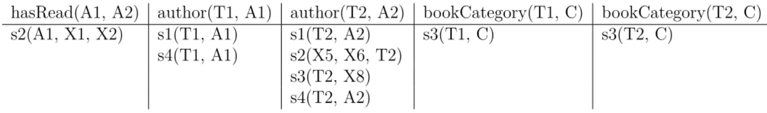
For query given in Listing 4.10, and views in Listing 4.11, the algorithm builds five buckets, one for each query subgoal as in Table 4.1.
For the second subgoal, author(T1, A1), the view s1(T1, A1) has been included as the mapping
ψ(A) = A1, ψ(T ) = T 1, makes s1 second subgoal author(T, A), equal to the query subgoal, and
distinguishable variable A1 in the query corresponds to distinguishable variable A in the view. But view s3(T1, X7) has not been included in this bucket because the variable A, distinguishable in the query, can only correspond to an existential variable in the view.
Table 4.1 – Buckets for query in Listing 4.10, and views in Listing4.11
hasRead(A1, A2) author(T1, A1) author(T2, A2) bookCategory(T1, C) bookCategory(T2, C) s2(A1, X1, X2) s1(T1, A1) s1(T2, A2) s3(T1, C) s3(T2, C)
s4(T1, A1) s2(X5, X6, T2) s3(T2, X8) s4(T2, A2)
In the second part of the Bucket algorithm [50, 34], the Cartesian product of the built buckets is considered. Each element of this Cartesian product is a possibly contained rewriting, having one element from each bucket to cover the corresponding query subgoal. Each possibly contained rewrit-ing should satisfy two conditions to be a valid contained rewritrewrit-ing: (i) they should be satisfiable; (ii) they should be contained in the query. Join predicates can be added to the possible rewritings in order to make them contained in the query.
Listing4.12 gives the eight possible contained rewritings. Rewriting r1 includes the first element of each bucket to cover the query subgoals, rewriting r2 includes the second element of the bucket for the third query subgoal, and the first element for all the other buckets. In r2 the same view (s2 ) is used to cover the first and third subgoals, while the r1 two different views, s2 and s1, are used to cover the first and third subgoals.
Listing 4.12 – Cartesian product of the buckets in Table4.1, these queries are the possibly contained query rewritings
r 1 ( A1 ) :− s 2 ( A1 , X1 , X2 ) , s 1 ( T1 , A1 ) , s 1 ( T2 , A2 ) , s 3 ( T1 , C ) , s 3 ( T2 , C ) r 2 ( A1 ) :− s 2 ( A1 , X1 , X2 ) , s 1 ( T1 , A1 ) , s 2 ( X5 , X6 , T2 ) , s 3 ( T1 , C ) , s 3 ( T2 , C ) r 3 ( A1 ) :− s 2 ( A1 , X1 , X2 ) , s 1 ( T1 , A1 ) , s 3 ( T2 , X8 ) , s 3 ( T1 , C ) , s 3 ( T2 , C ) r 4 ( A1 ) :− s 2 ( A1 , X1 , X2 ) , s 1 ( T1 , A1 ) , s 4 ( T2 , A2 ) , s 3 ( T1 , C ) , s 3 ( T2 , C )
r 5 ( A1 ) :− s 2 ( A1 , X1 , X2 ) , s 4 ( T1 , A1 ) , s 1 ( T2 , A2 ) , s 3 ( T1 , C ) , s 3 ( T2 , C ) r 6 ( A1 ) :− s 2 ( A1 , X1 , X2 ) , s 4 ( T1 , A1 ) , s 2 ( X5 , X6 , T2 ) , s 3 ( T1 , C ) , s 3 ( T2 , C ) r 7 ( A1 ) :− s 2 ( A1 , X1 , X2 ) , s 4 ( T1 , A1 ) , s 3 ( T2 , X8 ) , s 3 ( T1 , C ) , s 3 ( T2 , C ) r 8 ( A1 ) :− s 2 ( A1 , X1 , X2 ) , s 4 ( T1 , A1 ) , s 4 ( T2 , A2 ) , s 3 ( T1 , C ) , s 3 ( T2 , C )
All the possibly contained rewritings given in Listing 4.12 are satisfiable as there are no two predicates in the same query that can produce any contradiction. However, not all of them are contained in the query. The first query in Listing 4.12, r1, that uses view s2 to cover the first subgoal and view s1 to cover the third subgoal, is not contained in the query, q, given in Listing4.10. The condition imposed on the first and third query subgoals with the shared variable A2, cannot be satisfied by view subgoals in s2 and s1, because query variable A2 has been mapped to a non distinguishable variable in s2. On the other hand, r2, that uses s2 to cover the first and third query subgoals, can be contained in the query if the join predicates X2 = T2 and A1 = X5 are added to
s2. Adding the constraints imposed by these join predicates can be also done by replacing variables X2 and X5 by T2 and A1, furthermore, after replacing the variables one of the occurrences of view s2 can be safely removed. Notice that the difference among the queries given in Listing 4.12, may be subtle, as it is the case for r1 and r2. s2 is already present in r1 and it is only used to cover the first query subgoal, while in r2 it is used to cover both the first and third query subgoals.
From the eight possible contained rewritings given in Listing4.12, only the queries r2 and r6 are contained in q. Valid rewritings, after variable replacing and simplification, are given in Listing4.13. The maximally contained rewriting is r2 S
r6.
Listing 4.13 – q’s valid contained rewritings, r2 and r6, obtained from the queries given in Listing4.12
q ( A1 ) :− h a s R e a d ( A1 , A2 ) , a u t h o r ( T1 , A1 ) , a u t h o r ( T2 , A2 ) , b o o k C a t e g o r y ( T1 , C ) , b o o k C a t e g o r y ( T2 , C ) r 2 ( A1 ) :− s 2 ( A1 , X1 , T2 ) , s 1 ( T1 , A1 ) , s 3 ( T1 , C ) , s 3 ( T2 , C )
r 6 ( A1 ) :− s 2 ( A1 , X1 , T2 ) , s 4 ( T1 , A1 ) , s 3 ( T1 , C ) , s 3 ( T2 , C )
The MiniCon Algorithm
The MiniCon algorithm [65, 34] is an optimization of the Bucket algorithm that avoids the last verification step by a more complex first step. The MiniCon algorithm uses MiniCon Descriptors (MCDs) instead of buckets. The number of combinations of MCDs is considerably lower than for the buckets, and all the resulting rewritings are contained in the query by construction. For each query subgoal, if a view subgoal sgv covers a query subgoal sgq, all the query subgoals that share variables
with sgq are considered together, and further checking is done to assess that these query subgoals
may be covered by view subgoals in a compatible way. Then, a MCD is created and it includes the view head with the proper mapping, and the covered subgoals. To formally define MCDs, the term
head homomorphism is used. A head homomorphish h for view V is a variable mapping from the
variables in V to the variables in V , that is the identity on existential variables, but may make two distinguished variables equal.
Definition 9 (MiniCon descriptions [65]). An MCD C for a query Q over a view V is a tuple of the
form (hC, V ( ¯Y )C, ϕC, GC) where hC is a head homomorphism on V, V ( ¯Y )C is the result of applying
hC to V, i.e., ¯Y =hC( ¯A), where ¯A are the head variables of V, ϕC is a partial mapping from Vars(Q)
to hC(Vars(V)), GC is a subset of the subgoals in Q which are covered by some subgoal in hC(V)
using the mapping ϕC (note: not all such subgoals are necessarily included in GC).
If GC has the minimum size such that the conditions are satisfied, then a set of MCDs with
disjoint subgoals can be built, and the combination of MCDs is straightforward. Query rewritings are obtained by combining MCDs such that all the query subgoals are covered. In order to reduce the number of MCDs combinations, the MiniCon algorithm obtains MCDs that satisfy Property 1.
Property 1 (Property 1 [65]). Let C be an MCD for Q over V. Then C can only be used in a
non-redundant rewriting of Q if the following conditions hold:
C1 For each head variable x of Q which is in the domain of ϕC, ϕC(x) is a head variable in hC(V).
C2 If ϕC(x) is an existential variable in hC(V), then for every g, subgoal of Q, that includes x: (1)
all the variables in g are in the domain of ϕC ; and (2) ϕC(g) ∈ hC(V )
When Property 1 is ensured, then rewriting construction is easily done thanks to Property 2.
Property 2 (Property 2 [65]). Given a query Q, a set of views V, and the set of MCDs C for Q
over the views in V, the only combinations of MCDs that can result in non-redundant rewritings of Q are of the form C1,...,Cl, where:
D1 GC1 S . . . S GCl = Subgoals(Q), and D2 for every i 6= j, GCi T GCj = ∅
Algorithm2presents the first part of the MCD algorithm. Similarly to the Bucket algorithm, for each query subgoal, each view and its goals are considered to cover the query subgoal (lines 3-12).
Algorithm 2 MiniCon first part: form MCDs [65]
Require: Q : ConjunctiveQuery; V : set of View (defined as ConjunctiveQuery) Ensure: C: set of MCD
1: function formMCDs(Q, V)
2: C ← ∅
3: for all q ∈ body(Q) do
4: for all v ∈ V do
5: for all w ∈ body(v) do
6: if There is a mapping ϕ and head homomorphism on V, h, such that ϕ(q) = h(w) then
7: h ← the least restrictive homomorphism h such that ϕ(q) = h(w)
8: C ← CS{ (hC, V ( ¯Y )C, ϕC, GC) : h ⊆ hC∧ ϕ ⊆ ϕC ∧ (hC, V ( ¯Y )C, ϕC, GC) is minimal for Property1}
9: end if 10: end for 11: end for 12: end for 13: return C 14: end function
Head homomorphism h and mapping ϕ are looked up (line 6), and their extensions that satisfying Property 1cover the least number of query subgoals, are used to form the MCDs (line 8).
Proposition 2. The time complexity of Algorithm2 is O(nn× m × kn× ln), where n is the number of
query subgoals, m is the number of views, k is the maximum number of view goals, l is the maximum number of arguments per query or view subgoal.
The first part of the MiniCon algorithm has higher time complexity than the first part of the Bucket algorithm, as the variables from the set of query subgoals that share existential variables should be mapped to a set of view subgoal variables to satisfy C2 from Property1. But the overall complexity for both algorithms is the same: O((n×m×k)n), where n is the number of query subgoals,
m is the number of views, k is the maximum number of view goals, l is the maximum number of
arguments per query or view subgoal (and l is dominated by k) [65].
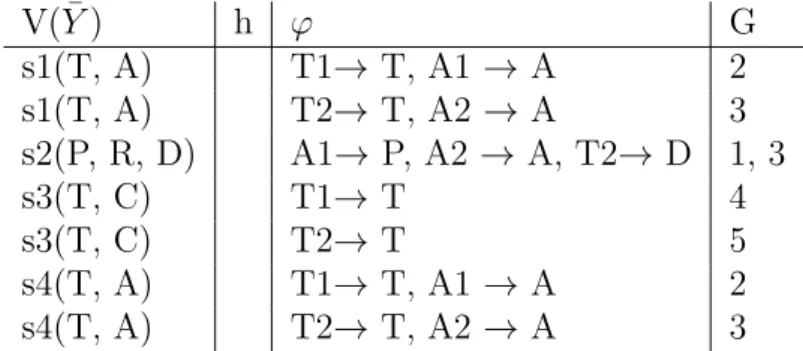
Table 4.2 – MCDs for query in Listing 4.10 and views in Listing 4.11, for h and ϕ identity part has been omitted, i.e., h(X) = X (ϕ(X)=X) for any other variable in the domain of h (ϕ)
V( ¯Y ) h ϕ G s1(T, A) T1→ T, A1 → A 2 s1(T, A) T2→ T, A2 → A 3 s2(P, R, D) A1→ P, A2 → A, T2→ D 1, 3 s3(T, C) T1→ T 4 s3(T, C) T2→ T 5 s4(T, A) T1→ T, A1 → A 2 s4(T, A) T2→ T, A2 → A 3
For the query given in Listing 4.10, and the views in Listing4.11, the MiniCon algorithm builds four MCDs, as depicted in Table 4.2. For view s4, two MCDs have been built, one for the fourth subgoal and another for the fifth subgoal, as variable C in view s4 is distinguishable and joins on
that variable can be enforced without having to cover both subgoals in the same MCD. Notice that no MDC has been built for view s3 and the third subgoal. View s3 is not included for the third subgoal because variable A2 is existential in the view and the view does not cover all the query subgoals that involve the variable A2.
Listing 4.14 – Valid contained rewritings, r1 and r2, obtained from the combination of MCDs in Table 4.2
q ( A1 ) :− h a s R e a d ( A1 , A2 ) , a u t h o r ( T1 , A1 ) , a u t h o r ( T2 , A2 ) , b o o k C a t e g o r y ( T1 , C ) , b o o k C a t e g o r y ( T2 , C ) r 1 ( A1 ) :− s 2 ( A1 , X1 , T2 ) , s 1 ( T1 , A1 ) , s 3 ( T1 , C ) , s 3 ( T2 , C )
r 2 ( A1 ) :− s 2 ( A1 , X1 , T2 ) , s 4 ( T1 , A1 ) , s 3 ( T1 , C ) , s 3 ( T2 , C )
Listing 4.14 presents the only two valid contained rewritings obtainable from the MCDs in Ta-ble 4.2, these rewritings are equivalent to the rewritings given in Listing 4.13, and obtained using the Bucket algorithm.
MCDSAT and SSD-SAT
MCDSAT [10] is a logic based method to produce MiniCon Descriptors (MCDs) and rewritings as translations of models for logical theories. These theories, called MCD theory and extended theory, model the rules that any MCD or rewriting must satisfy. These theories are compiled into d-DNNFs [24], i.e., deterministic, decomposable negation normal form, for which model counting can be done in polynomial time. This query rewriter benefits from existing d-DNNFs compilers to produce rewritings faster than the traditional MiniCon implementation [10].
Izquierdo et al [40] extend the MCDSAT rewriter with constants and preferences to identify the combination of semantic services that rewrite a user request. The expressive power of this extension is greater but also is the complexity of the logical theories.
Graph-based Query Rewriting (GQR)
Graph-based Query Rewriting (GQR) [44] models query and view subgoals as graphs. These graphs abstract from variable names, and a preprocessing step is performed over the views to com-pactly represent all the views with few graphs. Then, when a query is posed, for each query subgoal relevant graphs are selected, and graphs are incrementally combined in order to produce larger graphs that cover more query subgoals. The view graphs correspond to partial rewritings, and differently from previous rewriters, rewritings may be produced incrementally as the partial rewritings are
![Figure 7.1 – Distributed Query Processing, Figure 6.3 at [62]](https://thumb-eu.123doks.com/thumbv2/123doknet/7799745.260811/67.892.258.622.92.525/figure-distributed-query-processing-figure-at.webp)
