Dionne : HEC Montréal, 3000 Chemin de la Côte-Sainte-Catherine, Montréal, Québec, Canada H3T 2A7. Phone : +514 340-6596; Fax : +514 340-519; and CIRPÉE
georges.dionne@hec.ca
Maalaoui Chun : KAIST, Graduate School of Finance, 87 Hoegiro, Dongdamoongu, Seoul, South Korea, 130-722. Phone : +822 958-3424; Fax : +822 958-3180
olfa.maalaoui@gmail.com
Presidential address of Georges Dionne at the Canadian Economics Association Meetings, Montreal, June 1, 2013. Georges Dionne thanks École Polytechnique in France for its hospitality during the writing of different versions of this article. Both authors thank Albert Lee Chun, Mohamed Jabir, and Claire Boisvert for their generous help. Comments from Linda Allen, David Green and an anonymous referee were very useful to improve the previous versions.
Forthcoming at the Canadian Journal of Economics
Cahier de recherche/Working Paper 13-22
Default and Liquidity Regimes in the Bond Market during the
2002-2012 Period
Georges Dionne
Olfa Maalaoui Chun
Abstract:
Using a real-time random regime shift technique, we identify and discuss two different
regimes in the dynamics of credit spreads during 2002-2012: a liquidity regime and a
default regime. Both regimes contribute to the patterns observed in credit spreads. The
liquidity regime seems to explain the predictive power of credit risk on the 2007-2009
NBER recession, whereas the default regime drives the persistence of credit spreads
over the same recession. Our results complement the recent dynamic structural models
as well as monetary and credit supply effects models by empirically supporting two
important patterns in credit spreads: the persistence and the predictive ability toward
economic downturns.
Keywords: Credit spread, credit default swaps, real-time regime detection, market risk,
liquidity cycle, default cycle, credit cycle, NBER economic cycle
I. Introduction
This paper focuses on the identification of liquidity and default regimes in the bond market during the 2002-2012 period, which covers the recent financial crisis and the 2009 NBER eco-nomic recession. The recent literature has assumed a strong link between the business cycle and the credit cycle (e.g. Hackbarth, Miao, and Morellec, 2006; Chen, 2010; Bhamra, Kuehn, and Strebulaev, 2010; Giesecke, Longstaff, Schaefer, and Strebulaev, 2011; Bhamra, Fisher, and Kuehn 2011; Dionne et al., 2011). Yet empirical evidence supports only the presence of an imperfect overlap between the credit cycle and the economic cycle. The credit cycle en-compasses the entire recessionary period but often extends beyond the end of the recession. Nonetheless, the observed patterns of the credit cycle have to be explained using its main two drivers: the default cycle and the liquidity cycle. It would be interesting to know how these cycles behave during periods of financial distress and recession. Specifically, our main objective is to explain regime shifts in the credit risk factor of bond spreads by thoroughly analyzing these shifts in the default factor and in the liquidity factor.1
Maalaoui Chun, Dionne and François (2013) show that corporate bond spreads describe a long-lasting level regime that contains but outlasts NBER recessions. They also argue that regime shifts (especially for high-yield bonds with short maturities) are often detected before the effective starting date of the NBER economic recession. An important component in the credit regime stems from high default premiums observed during recessions. The empirical evidence also suggests that credit regimes contain a factor that qualifies as a forward-looking measure of financial and economic downturns.
In addition, the authors link their credit regimes to two economic indicators: the Senior Loan Officer Opinion (SLO) Survey, which captures capital market liquidity, and the Fed fund rate, which captures the state of monetary policy. The detected credit regime is almost always affected by credit supply effects but has feedback effects with monetary policy actions. Thus, the dynamics of the credit regime may result from changing liquidity conditions in the bond market.
Longstaff, Schaefer, and Strebulaev (2011) find that, since the railroad crisis in 1873-1875, historical patterns of default have constituted important economic phenomena that often repeat themselves. Longstaff, Mithal, and Neis (2005, LMN) support the idea that the default risk is the most important part of the corporate credit spread, using data before the financial crisis (2000-2001). However, Dick-Nielsen, Feldhutter, and Lando (2012, DFL) reach a different conclusion for the recent subprime crisis. They argue that since the onset of the subprime crisis, most of the credit spread has been due to the illiquidity of the bond market. This confirms the need to re-examine the relationship between default and liquidity risk in the bond market by modeling these risks distinctly and linking them to the credit risk premium (Han and Zhou, 2008).
We estimate the default risk of corporate bonds using information from credit default swap (CDS) contracts. The CDS contracts have the advantage of being more liquid than corporate bonds and thus embed new information concerning changes in the creditworthiness of the issuer more efficiently.2
Thus, a CDS premium is a timely reflector of the credit worthiness of the firm that issued the bond. Further, given that CDS are contracts rather than securities, the premium of a CDS contract is much less sensitive to effects of liquidity and market risks and effects of convenience yield than are corporate bond prices. Thus, CDS contracts are attractive from the point of view of estimating default risk. We closely follow LMN in constructing the individual default risk measure for each firm in our sample. Our study covers the period from 2002 to 2012, a much larger window than the 2000-2001 period in LMN (2005) or the 2005-2009 period in DFL (2012). As opposed to only considering the single 5-year CDS contract, following Chun and Yu (2013) we also analyze the whole term structure of CDS contracts for each firm when filtering out the firm-specific default risk measure.
To measure the liquidity premium we use the most comprehensive source of high fre-quency bond transactions provided by TRACE. We follow Han and Zhou (2008) and Dick-Nielsen, Feldhutter, and Lando (2012) in measuring the liquidity component for each firm in our sample using several measures of liquidity. Relative to these contributions, our study covers the entire 2007-2009 financial crisis, the recent 2007-2009 NBER recession, as well as the aftermath period of the crisis (2009-2012), This allows us to study the characteristics of corporate bonds during an important period of recovery and debt restructuring. Finally, using the real-time regime detection technique of Maalaoui Chun, et al (2013), we extract distinct regimes of default and liquidity risk for the sample of firms in our study and contrast them with the credit risk regimes.
Our results show that, for corporate bonds, a first liquidity risk shift occurred at the begin-ning of the financial crisis period (07-2007) and a second more important shift occurred near the middle of the crisis period (06-2008). This second high-liquidity regime persists until the end of the financial crisis in 03-2009. This means that the first liquidity regime shift predates the NBER recession (12-2007 to 06-2009), as is the case with the date of the first corporate credit risk shift (09-2007). In fact, it is this first liquidity risk shift that seems to drive the predictive power of the credit risk shift on the 2007-2009 NBER recession.
Regarding the default risk regimes, an important regime shift occurred in June 2008, well after the beginning of both the financial crisis and the NBER recession starting date. The persistence of the default risk factor following both periods is much stronger than the persis-tence of the liquidity risk factor, which is in line with results found in the recent theoretical literature on dynamic structural default risk models (Hackbarth, Miao, and Morellec, 2006; Chen, 2010; and Bhamra, Kuehn, and Strebulaev, 2010). Our results also support monetary
2Detailed discussions on the differences between CDS premiums and corporate bond spreads can be found in
and credit supply effects models of Bhamra, Fisher and Kuehn (2011), Bernanke and Gertler (1989), King(1994), and Kiyotaki and Moore (1997).
The remainder of this paper is organized as follows. The next section reviews the credit risk literature by emphasizing two major components of credit risk – default risk and liquidity risk. Section III briefly outlines the model used to extract default risk from the information in CDS contracts. It also outlines the model used to measure liquidity risk and the regime shift detection technique. Section IV describes the TRACE data for bond transactions as well as the Markit data that includes all North American Financial CDS data for CDS contracts. Section V presents the results. Section VI concludes the paper. Technical details are reported in the Appendix.
II. Literature review
II.1 Credit risk models
Credit risk in this paper is referred to as the yield spread, i.e. the difference between the yield of a defaultable bond and the yield of the government bond with the same maturitiy (Duffee, 1998). This difference, also called a credit spread in the literature, measures the risk premium associated with the credit risk. This means that corporate bond investors ask for a higher yield on a corporate bond because they are exposed to additional risks and costs that do not affect a government bond (or any other equivalent benchmark; see for instance Hull et al., 2004). We assume that the government bond yield does not contain any premium related to currency devaluation, public debt or public deficit and liquidity (Ejsing, Grothe and Grothe, 2012). In other words, we do not cover the risk of sovereign debt. However, bonds issued by firms, financial institutions and the government can all be affected by market risk (Fama and French, 1993).
Two important research questions in the recent financial literature are : 1) What portion of corporate yield spreads is directly attributable to default risk? and 2) How much of the corporate yield spread stems from other factors such as liquidity risk, tax, risk aversion, mar-ket risk, and macroeconomic risk? (Elton et al., 2001; Colin-Dufresne et al., 2001; Lando and Skodeberg, 2002; Huang and Huang, 2003; Driessen, 2005; Chen, Collin-Dufresne and Gol-stein, 2009; Dionne et al., 2010; among others). These issues are of fundamental importance from an investment perspective because corporate debt is one of the largest asset classes in financial markets (Longstaff et al., 2005). They are also important from a macroeconomic point of view because yield spreads are closely linked to business and monetary cycles. If credit spreads predict business cycles, it would be interesting to determine which its com-ponents is driving this predictive power. Finally, during the recent financial crisis, liquidity risk became important, especially in the banking industry. During that period, liquidity risk was significant for many financial assets (such as asset-backed commercial paper (ABCP) in Canada), and central banks had to use special policy measures to inject liquidity into the
financial system. Finally, the new international regulatory framework for banks (Basel III, 2010) emphasizes the role of liquidity risk in computing regulatory capital.
Since the beginning of the 2000s, the finance literature has distinguished between default risk and credit risk. Default risk is the risk that a bond issuer will not be able to pay the agreed coupons and principal during the life of the corporate bond. Default risk contains three main elements: 1) the probability of default (PD) and the related bond rating migration (BRM); 2) the expected value of the bond at default (EAD); and 3) the loss given default (LGD), which is the fraction of EAD that will not be recovered by the bondholder after default.
Before the 2000s, credit risk was considered as synonym to default risk. Yet, research has shown that credit risk cannot be explained only by historical default related variables. The default risk represents only a fraction of corporate credit spread which instantaneously represent the premium according to structural models. Even by adding additional candidates further suggested by more recent structural models, the literature has been able to explain around 25% to 85% of the yield spread, depending on the bond rating, the period considered, the nature of the data available, and the set of factors considered including the business cycle (Elton et al., 2001; Colin-Dufresne et al., 2001; Huang and Huang, 2003; Lando and Skodeberg, 2002; Dionne et al., 2010; Maalaoui-Chun, et al, 2010; Cenesizoglu and Essid, 2012). This phenomenon is now labeled as the Credit Risk Puzzle.
Liquidity risk has been documented as one of the important determinants of corporate bond credit spreads (e.g. Longstaff, Mithal, and Neis, 2005). Yet, the lack of transaction bond data necessary to measure this risk limited the empirical support of this hypothesis. During the recent financial crisis many structured financial products such as asset-backed commercial paper (ABCP) and collateralized debt obligations (CDO) became highly illiquid supporting the idea that liquidity risk is an important risk in the credit market.
The macroeconomic risk factor is also an important determinant of credit spread. A statis-tical link between business cycles and credit spread levels and volatility has been observed, however the causality between the business cycle and the credit cycle is not well established. For instance, as documented by Maalaoui-Chun, et al (2013), and Ng, (2013), there is no per-fect concordance between business cycles and credit cycles. Credit cycles last often longer than business cycles. When recessions officially end, corporate yield spreads remain high for many months, meaning there is persistence in credit cycles. More importantly, because cor-porate bond spreads start to increase before economic recessions they can even be viewed as predictors of recessions.
Early contributions on decomposing credit spreads have been limited by the availability of bond data. Today, detailed data on bond transactions at high frequency become available. In addition, a larger set of credit derivatives is traded actively in financial markets providing researchers with alternative data sources to examine the dynamics of corporate yield spreads more closely.
of default and non-default components in corporate yield spreads. They assume that the CDS premium is an appropriate measure of default risk. A CDS is like an insurance contract that compensates the investor for losses arising from the default of a corporate bond. In such contracts, the owner of a corporate bond is the party buying protection by paying the seller of a CDS (usually an investment bank or an insurer) a fixed premium each period (usually a quarter) until either the bond defaults or the swap contract matures. In return, if the underlying firm defaults on its debt, the protection seller is obliged to buy the defaulted bond back from the CDS buyer at its par value. The protection seller usually loses a fraction (LGD) of the par value of the defaulting bond.3
LMN (2005) find that more than fifty percent of corporate yield spread is due to default risk. This result holds for all studied rating categories and is robust to the definition of the riskless curve. In particular, using credit spreads over Treasury yields, the default component represents 51% of the spread for AAA and AA rated bonds, 56% for A-rated bonds, 71% for BBB-rated bonds, and 83% for BB-rated bonds. These results contrast with those in Elton et al. (2001) and Huang and Huang (2003), who report that default risk accounts for only about 25% of the spread for investment-grade bonds, but they are similar to the findings of Dionne et al. (2010, 2011).
Using Treasury bond yields as a benchmark to compute credit spreads, LMN (2005) find evidence of a significant non-default component for every firm in the sample. This non-default component ranges from about 20 to 100 basis points. They argue that the non-default com-ponent of corporate bond spread is time varying and strongly related to measures of bond-specific illiquidity as well as to macroeconomic measures of bond market illiquidity, such as the size of the bid/ask spread and the principal amount outstanding of corporate bonds.
Dick-Nielsen, Feldhutter and Lando (DFL, 2012) show how the increase in corporate bond spreads during the subprime crisis can be attributed to escalating bond illiquidity. As a mea-sure of illiquidity, they used an equally weighted sum of four liquidity variables normalized to a common scale and identified from principal component analysis. The four liquidity vari-ables are measured quarterly and include the Amihud’s measure of price impact, a measure of roundtrip cost of trading and the variability of the two measures. To analyze variations in credit spreads they considered different control variables such as default risk, taxes, and the general economic environment. Yet, they did not use CDSs sold on these bonds to measure default risk. The main conclusion in DFL work is that liquidity risk become very important after the subprime crisis especially for investment grade bonds. For speculative grade bonds, the total spread explained by liquidity risk was 24% during the pre-subprime period and 23% during the post-subprime crisis. However, for investment grade bonds, the ratio increased significantly between the two periods ranging from 3% to 8% during the pre-subprime period (according to the ratings) to 23% to 42% during the post-subprime crisis. The exception is AAA
3There are other equivalent settlement methods in the market that we do not discuss in our analysis (Lando,
bonds, which varied from 3% to 7% between the two periods. They attribute this exception to a fly-to-quality phenomenon. They also obtained different results when considering bonds with different maturities with the largest variations between the pre and post subprime observed for bonds with 10 to 30 years of maturity.
DFL also looked at the effect of the nature of the bond underwriter and the industry origin on bond illiquidity. Specifically, they analyzed the illiquidity of bonds underwritten by Bear Stearns and Lehman Brothers and compared them with the illiquidity of bonds underwrit-ten by other banks. They found a small effect for Bear Stearns, which was acquired by J.P. Morgan. However, they document a big jump in the illiquidity index of bonds underwritten by Lehman Brothers during the period around the default of the bank followed by some per-sistence after the bankruptcy date (September 15, 2008). By comparing the illiquidity index of bonds of industrial firms with the index of bonds of financial firms, they find that bonds of financial firms were more liquid before the onset of the financial crisis in July 2007 and became less liquid after that date. In conclusion, these authors observed that bond spreads increased considerably during the financial crisis and found that bond illiquidity contributed significantly to that widening.
Chiaramonte and Casu (2013) analyze the determinants of CDS spreads during the period 01-01-2005 to 30-06-2011, including the financial crisis of 01-07-2007 to 31-03-2009. The model is limited to bank-specific balance sheet ratios as possible determinants of the spreads. Their results indicate that Tier 1 capital and leverage are not significant over the period of analysis, while liquidity indicators are significant only during and after the financial crisis period. Liquidity is measured by two ratios: 1) Net loans/ deposits and short-term funding (%), and 2) Liquid assets/deposits and short-term funding (%). Interestingly, during the financial crisis only the first definition of liquidity is significant reflecting the high leverage in the credit market. However, in the post-crisis period both definitions of liquidity become significant. According to these results, the authors argue that liquidity risk become a major concern since Basel III.
Recent papers have analyzed the speed of convergence to stable liquidity conditions in the stock market. For instance, following a liquidity shock, how many quote updates are neces-sary for transaction costs or market depth to return to their pre-shock levels? (Degryse et al. 2005; Wuyts, 2012; Foucault et al., 2005). In the same spirit, Beaupain and Durré (2013) analyze the resilience in the money market.4 They examine the determinants of the spread between the overnight interest rate and the European Central Bank (ECB) policy rate. By definition, this spread is affected only by market liquidity conditions. In resilient markets, liquidity shocks should be absorbed without affecting prices. Further, resilient markets at-tract market participants and favor trading thus speeding up convergence to stable liquidity conditions in periods of liquidity distress. Beaupain and Durré (2013) main results identify
4According to Kyle (1985) liquidity is related to 1) tightness (transaction costs), 2) depth and 3) resiliency of
liquidity, market activity and the institutional setting of the ECB’s refinancing operations as significant determinants of the observed resiliency regimes. They also show how the speed of mean reversion of market liquidity affects the yield curve in the euro zone. Finally, these results highlight the interplay between the money market and the central banks and their role in efficiently providing banks with stable liquidity conditions in both normal and stress periods around the financial crisis.5
II.2 Liquidity risk and default risk during the 2007-2009 financial crisis
To interpret our statistical results we briefly chronicle the major events during the recent fi-nancial crisis. Difficulties started in the United States when housing prices began to decrease in 2006 following a rapid increase in interest rates intended to reduce inflation. Many home owners who contracted subprime loans went bankrupt. Because these loans were transferred to financial markets via securitization, banks did not screen and monitor these risks carefully. Loans were allowed without down payments and with little analysis of borrowers’ credit ca-pacity and income. Moreover, the excessive use of short-term funding and the increased use of CDSs concentrated risk within a few big financial institutions (Bernanke, 2013; Saunders and Allen, 2010).
The US government and the Federal Reserve did not control the financial system ade-quately during that mortgage crisis period. No concrete action was taken to reinforce banks’ monitoring and managing of their different risks, and to compel them to hold adequate capi-tal. The Federal Reserve also did not fully play its role in ensuring the stability of the financial system. The source of the problem was mainly related to the non-transparency of the struc-tured financial markets and poor risk management of strucstruc-tured financial products (Dionne, 2013). Nobody knew where structured assets such as ABCP and CDOs were sold via OTC (Over-The-Counter Transactions); and who would incur the losses, thus creating great uncer-tainty in financial markets (Acharya et al 2013; Bernanke, 2013; Saunders and Allen, 2010).
Many regulatory failures accelerated the crisis. The rollover of ABCP, issued by Special Investment Vehicles, was supposed to be financed and guaranteed by commercial banks. How-ever, such guaranties did not exist because they were not required by the regulation. In fact, many ABCP issues were not adequately documented (Chant, 2008, 2013). Moreover, dur-ing the crisis, banks sustained severe losses and the market value of their equity collapsed. These banks continued to pay dividends instead of keeping capital because, according to the regulatory standards, they were well capitalized (Acharya, 2013).
Banks were rapidly exposed to liquidity risks during the financial crisis (Acharya et al
5Stulz (2010) reviews the role of CDSs during the financial crisis. Allen et al, (2011) show that during the crisis,
there was no variation in short-term spreads for Canadian financial institutions, although the 5-year CDS spreads varied substantially during the same period. They conclude that CDSs may not be appropriate instruments for providing information in very short periods of time. On the other hand, Chen et al, (2011) show there is strong interactions between interest rate risk and default risk measured by the term structure of CDSs with US data in a period preceding the financial crisis (2003-2007). See also Zorn et al. (2009) who document the interventions of the Canadian federal government in response to the financial crisis.
2012). The liquidity crisis started during the summer of 2007. Banks were committed to credit lines that borrowers and structured product issuers could use at any time. Indeed, many firms and consumers used their credit line opportunity to reduce the effects of the crisis on their own portfolios. As a result, banks had less money for new lending. The repo market also failed during the financial crisis. Banks that used the repo market to finance purchases of structured products had two options: sell good quality securities in a down market or find expensive sources of credit to replace the repo market . These activities are the early indicators of a liquidity shortage in the financial market. Finally, the financial crisis accelerated when investors exercised the option not to roll over the short-term debt (Acharya, 2013).
The liquidity crisis turned into a default crisis in 2008. The nearly bankrupt bank Bear Stearns was sold to J.P. Morgan Chase with the help of the Federal Reserve. After failing to obtain a government bailout, the Lehman Brothers bank went bankrupt on September 15, 2008. That same day Merrill Lynch, another bank in financial difficulty, was acquired by Bank of America. The American Insurance Group (AIG), one of the biggest insurers in the world, was heavily involved in the CDS market and also had liquidity problems. It took several bailouts from the Federal Reserve to prevent its failure, yet this drove the economy into a deeper systemic downturn. A few days later, Washington Mutual was acquired by J.P. Morgan Chase bank, and Wachovia was taken over by Wells Fargo. During that period the Federal Reserve had to play its role of lender of last resort and provide liquidity to the financial market to stabilize the crisis (Bernanke, 2013).
Thus, in line with Saunders and Allen (2010), the period of the recent financial crisis can be decomposed into three major phases on which we base our empirical results. The first period characterizes the credit crisis in the mortgage market (06-2006 to 06-2007), the second period covers the period of the liquidity crisis (07-2007 to 08-2008), and the third period refers to the default crisis period (09-2008 to 03-2009). In this study we are mainly concerned with the second and third periods.
III. Models
In this section we present three models that will be used to decompose credit spread shifts into default shifts and liquidity shifts during the 2002-2012 period. We first present the default spread model where the spread is measured by the CDS premium of the corporate bonds, as in Longstaff et al (2005) and Chun and Yu (2013). Then we follow Dick-Nielsen et al’s (2012) methodology to obtain an empirical measure of the bond illiquidity component of corporate bond spreads. Finally, we present the regime shift model of Maalaoui Chun et al (2013) that will be used to compare the regime shift periods of credit, default and liquidity risk in relation to the last financial crisis (07-2007 to 03-2009) and NBER recession (12-2007 to 07-2009).
III.1 The default premium of the debt issuer
Default risk is the risk of reduction in bond market value caused by changes in the quality of bond issuers. This risk represents the fraction of the change in corporate bond yield spread as-sociated with default risk. This fraction can be measured by the CDS premium on a corporate bond.6
A CDS is a financial instrument that provides insurance against the default of a reference security (the bond) or the reference credit (the issuer of the bond). A simple illustration of the CDS contract involves a protection buyer (the buyer of CDS protection) and a protection seller (the seller of CDS protection). The protection buyer buys protection against the default of the reference bond or of its issuer by taking a long position on the CDS contract. The protection buyer pays a periodic CDS premium to the protection seller until either the default of the reference entity occurs or the CDS contract reaches maturity.7
If default of the reference entity occurs before the maturity of the CDS contract, the pro-tection seller buys the defaulted bond from the propro-tection buyer at its face value. As noted by LMN in practice it is very common to assume that the CDS premium equals the default component of the bond issuer’s credit spread.8Using the reduced-form approach developed by
Duffie and Singleton (1999, 2003), we represent the firm-specific intensity of default implied by the observed premium in a CDS contract.
The risk-neutral default intensity of the corporate bond follows a square-root diffusion (Cox-Ingersoll-Ross, 1985, CIR) process :
d it= i i it dt + i
q
i
tdZti: (1)
where iis the intensity of the Poisson process governing the default of the reference issue i; Zi is a standard Brownian motion, and i; i; i are CIR parameters capturing the dynamics
of the default intensity of the reference issue i. We follow Chun and Yu (2013) and use the Kalman Filter approach to infer for each reference issue i the CIR parameters corresponding to the whole observed term structure of CDS premia.9 We assume that the default-free
inter-est rate that we denote rtis independent of it. As documented in LMN, this assumption has
little effect on the empirical results, and it greatly simplifies the model. Suppose firm i may default at time i. Thus, at this time i; the bondholder recovers a fraction (1 wi) of the par
6Another method of measuring default risk is to compute its components (default probability (DP), exposure
at default, (EAD) and loss given default (LGD)) directly by using bond data (Elton et al, 2001; Lando et al, 2002; Dionne et al, 2010).
7The International Swaps and Derivatives Association has defined six credit events that trigger settlement
un-der the CDS contract. These events include bankruptcy of the reference entity, failure to pay interest or principal when due, debt restructuring unfavorably affecting the credit holder, obligation default, obligation acceleration, and repudiation/moratorium.
8We do not consider counterparty risk of CDS writers although some of them had solvency problems during
the recent financial crisis. Since we are mainly interested in the study of regime shifts, this should not affect our results significantly.
9
value of the bond. Suppose the protection buyer makes quarterly payments of si s4i on the
CDS at times 0; t1; ; tn until the maturity of the contract or the default event, whichever
comes first. Thus, we can write the present value of the premium leg of the CDS P (si; T ) as
follows: P (si; T ) = E tn X ti=1 e R0tirsds1 f i>tigsi ! : (2)
The independence assumption between rtand itallows us to rewrite Equation (2) as:
P (si; T ) = si tn X ti=1 E e R0tirsds E e R0ti itds ; (3) = si tn X ti=1 D(ti)E e Rti 0 itds ;
where D (ti) is the discount factor, i.e. the price of a nondefaultable zero-coupon bond with
maturity ti and face value of $1. In case of default at time i, the recovery on the reference
entity per unit of par value is (1 wi) so that the protection seller pays wi in default. The
value of the protection leg can then be expressed as follows:
P (wi; T ) = E e R i 0 rsds1 f i tngwi ; (4) = wi Z tn 0 E e R0irsds E te Rt 0 sds dt = wi Z tn 0 D(ti)E te Rt 0 sds dt;
where 1 is the default indicator. Following LMN, we rewrite Equation (3) and Equation (4) in terms of the diffusion parameters in Equation (1). It follows that:
P (si; T ) = si tn X ti=1 D (ti) Ai(ti) eBi(ti) i 0; (5) P (wi; T ) = wi Z tn 0 D (ti) Gi(ti) + Hi(ti) i0 eBi(t) i 0dt;
where Ai(ti), Bi(ti), Gi(ti), and Hi(ti) are expressed in terms of the CIR parameters ( i; i; i)
in Equation (1) and their functions A, B, G, H are given in the Appendix.
Given that the CDS contract has zero net value at inception, we can express the CDS premium si in terms of the default intensity i0 by equating the values of the two legs in the
CDS contract si= wiPnti=1D (ti) Gi(ti) + Hi(ti) i 0 eBi(ti) i 0 Pn ti=1D (ti) Ai(ti) e Bi(ti) i0 : (6)
where all parameters are as defined above.10 If i0is not stochastic, si = i0 wi, the expected
loss of the corporate bond. Otherwise, siis the weighted present value of i0 wi and is lower
than i0 wibecause of the negative correlation between i0and eBi(ti)
i
0 The expression in (6)
allows us to estimate the firm specific default intensity i0 using the whole term structure of observed CDS premia.
III.2 The liquidity premium of the issuer
The literature maintains that the concept of liquidity has several dimensions, which cannot be summarized using a single measure of illiquidity. We follow DFL and construct the eight illiquidity measures defined in their study and use principal component analysis to specify a common illiquidity factor that will be used to approximate the liquidity premium of corporate bonds.11
The Amihud illiquidity measure This measure is defined by Amihud (2002) as the aver-age ratio of the daily absolute return to the dollar daily trading volume. It characterizes the daily price impact of the order flow, i.e., the price change per dollar of daily trading volume. For each individual bond i, we compute the daily Amihud measure as follows:
Amihudit= 1 Nt Nt X j=1 1 Qij;t Pj;ti Pj 1;ti Pj 1;ti ; (7)
where Nt is the number of returns in each day t, Pj;ti (in $ of $100 par) denotes the jth
trans-action price of bond i in day t and Qi
j;t (in $ million) the jth trading volume of bond i in day
t. This measure reflects how much prices move due to a given value of a trade. Thus, a very illiquid bond would have a very high Amihud measure. To construct the Amihud daily mea-sures, we first apply the Han and Zhou (2008) filters. Specifically, we exclude transaction prices less than $1 and higher than $500. We exclude prices that are 20% higher than the median price of the same day or the previous day. We also exclude prices that are 20% lower than the median price of the same day or the previous day. After applying this filter, we verify that we have at least three transactions for each bond to obtain the daily Amihud measure. To obtain the monthly measures we take the median of daily measures.
10When default occurs between two payment dates, the protection leg value should be adjusted to account for
the accrued payment.
11
These illiquidity measures are commonly used in the literature. See Chen, Lesmond, and Wei (2007), Amihud (2002), Han and Zhou (2008), Feldhüter (2008), among many others.
The Imputed Roundtrip Cost This second measure of illiquidity, introduced by Feldhüter (2009), is constructed to capture transaction costs in imputed roundtrip trades (IRC). The imputed roundtrip cost (IRC) is defined as
IRC = Pmax Pmin Pmax
(8)
where Pmax and Pmin denote the maximum and minimum trading prices during a unique
roundtrip trade. The idea behind this measure is as follows. When during the same day a bond with the same volume trades two or three times but does not trade again at the same volume on that day, the trade is considered part of an imputed roundtrip trade. Thus, in the imputed roundtrip trade, the difference between the highest and lowest transaction prices reflects the transaction fees of the dealer or the bid-ask spread for that trade. For each day, we estimate the IRC as the average of daily estimates of IRC for different transaction volumes.
The Amihud liquidity risk and the IRC liquidity risk These two liquidity risks are measured through the standard deviation of the Amihud measure and the imputed roundtrip cost (IRC) respectively. The two measures capture the variability of bond illiquidity, yet pro-vide a sense of possible future illiquidity levels. We construct the daily liquidity risk measures using a rolling window of 21 trading days. To obtain monthly measures, we take the average across the month.
The Roll measure of the bid-ask spread Before November 2008, there was no indicator for whether the observed transaction price was a bid or an ask price. As a substitute, we use the implicit bid-ask spread measure following Roll (1984) over the 2002-2012 period. Un-der certain assumptions, the Roll measure infers the effective bid-ask spread directly from transaction prices:12
Rollit= 2 q
cov( Pi
t; Pt 1i ): (9)
where P denotes changes in transaction prices. The daily Roll measure is calculated using a rolling window of 21 trading days with at least four transactions in the window to be sure the measure is well-defined.
The average holding time of a bond We measure trading intensity using the daily turnover:
turnovert= total trading volumet
amount outstanding (10)
The turnover captures the trading intensity, which specifies assets that trade more fre-quently and thus are more liquid. The inverse of turnover (turnovert) can be interpreted as
12
The Roll measure is based on the assumption of market efficiency. It also assumes that the probability distribution of observed price changes within a very short period is stationary (i.e. two months).
the average holding time of a bond, which is another measure of illiquidity.
Bond’s zero trading days Another measure of non trading intensity is the ratio of the number of zero trading days over the total number of days during a period. Thus, a higher ratio indicates that the corporate bond is less liquid. We obtain the daily zero-trading days measure using a rolling window of 21 trading days.
bond zerot= number of bond zero trades within the rolling window
number of days in the rolling window (11)
Firm’s zero trading days Another measure of non-trading intensity is the firm’s zero trad-ing days, which counts the days in which none of the firm bond issues is traded in that day. Similar to the bond zero trades measure, we obtain the daily firm zero trades measure using a rolling window of 21 trading days.
firm zerot=
number of firm bonds zero trades within the rolling window
number of days in the rolling window (12)
The liquidity premium We construct a liquidity premium using the relevant loadings ob-tained from principal component analysis of the above illiquidity definitions. Specifically, the liquidity premium (or illiquidity factor) is a linear combination of illiquidity loads obtained from principal component analysis. We define each measure as litj; where i defines the cor-porate bond, t defines the day, and j defines the liquidity definition. Each measure is then normalized and leads to ljit = l
j it j
j ; with j and j defining the mean and the volatility of
the liquidity measure j across the different bonds and days. Finally, we define the daily mea-sure of the bond specific illiquidity factor as a linear combination of the normalized illiquidity measures. &it = J X j=1 ljit;
where J is the number of liquidity measures that will be retained from the principal com-ponent analysis.
III.3 Default and liquidity regime detection
The econometrics literature on structural changes provides a wide range of techniques for detecting break dates in time series.13 In this article we use the technique of Maalaoui Chun, et al (2013), which has the advantage of detecting possible break points in real time or when new data arrives. The non-parametric technique is a data-driven analysis in that it detects random regime shifts and can be classified among random regime models. It does not require
13See for instance Gordon and Pollak (1994), Bai and Perron (1998), (2003), Chib (1998), Chen, Choi, and Zhou
(2005), Perron and Qu (2006), Pesaran, Pettenuzzo, and Timmermann (2006), Davis, Lee, and Rodriguez-Yam (2008), Giordani and Kohn (2008), Maheu and McCurdy (2009), and Bai (2010).
any a priori assumptions about the timing or the number of detected regimes, and it does not require the regime to switch back to its previous level. Another feature of this technique is its ability to detect economic shocks affecting the level and the volatility of time series distinctly from one another. We can thus detect new regimes in the data and attempt to link these regimes to economic phenomena that remain unexplained.
Consider that data on a risk premium is represented by the following time series fYt; t =
1; :::; ng. Suppose Ytis described by an autoregressive model:
Yt ft= (Yt 1 ft 1) + "t; (13)
where ftcaptures a potentially time-varying mean, is the autocorrelation coefficient, and
"t N (0; 2). If time t = c is a breakpoint where the distribution of the data changes, then
the mean level ftcan be expressed as:
ft=
(
1; t = 1; 2; :::; c 1; 2; t = c; c + 1; :::; n:
(14)
where the null hypothesis for a shift at time c is performed using a two-sample t-test. The presence of a positive autocorrelation coefficient in equation (14), can generate false regime detections in the data. When the underlying data contain a stationary first-order autoregres-sive process with a positive autocorrelation coefficient, such a process is known as a red noise process. Thus, the removal of red noise, which involves estimating the AR(1) coefficient, is an important preliminary step that facilitates the accurate detection of regime shifts in the data. After the AR(1) coefficient is accurately estimated and the red noise is removed, the filtered time series is then processed with the regime shift detection method. (See Maalaoui Chun et al., 2013, for more details).
To detect a level regime, we start by defining the sample mean Zcur of the first sequence
of the data of length m.14 Let be the difference between the mean values of two subsequent
sequences that would be statistically significant at the level mean according to the Student
t-test:
= t2m 2mean q
2s2m=m; (15)
where m is the initial cut-off length of regimes similar to the cut-off point in low-pass filtering, s2mis the sample variance, and t2m 2
meanis the value of the two-tailed t-distribution with (2m 2)
degrees of freedom at the given probability level mean. During the test, the sample mean of
the current regime Zcur is known but the mean value of the new regime Znew is unknown:
The shift in the level occurs if the current value tested Zcur is outside the critical threshold
14
We previously check that the filtered data do not suffer from statistical issues related to the distribution of the data in each regime, heteroskedasticity of the residuals and square residuals. These issues are further discussed in Maalaoui Chun et al (2013).
i
Z#crit; Z"crith,
Z"crit= Zcur+ ; (16)
Z#crit= Zcur ;
where Z"critis the critical mean if the shift is upward and Z#critis the critical mean if the shift is downward. However, if the current value Zcur is inside the range
i
Z#crit; Z"crith, then we reject the null for a shift at tcur and we conclude that the current regime has not changed.
In this case, the value Zcur is included in the current regime and the test continues with the
next value. However, if the current value Zcuris greater than Z"critor less than Z#crit, the time
tcur is marked as a potential change point and the subsequent data are used to confirm or
reject this hypothesis using the Regime Shift Index (RSI) that represents a cumulative sum of normalized anomalies relative to the critical mean Zcrit:
RSI = 1 msm
j
X
i=tcur
Zi Zcrit ; j = tcur; tcur+ 1; :::; tcur+ m 1: (17)
If at any time during the testing period from tcur to tcur+ m 1 the RSI turns negative
when Zcrit = Z"crit or positive when Zcrit = Z#crit, the null hypothesis for a shift at tcur is
rejected. We include the value Zcurin the current regime and continue the test with the next
value at tcur = tm+ 2. Otherwise, time tcur is declared a change point and is significant at
least at the confidence level mean: The subsequent regime then becomes the current regime
and the test continues with the new data point.
IV. Data
In this research we use two main data sets.
The TRACE database: This database became available only in July 2002. The TRACE database reports high frequency data and contains information about almost all trades in the secondary over-the-counter market for corporate bonds, accounting for 99% of the total trading volume. Our data from TRACE cover the period from July 2002 to December 2012.15 We employ the filter proposed by Dick-Nielsen (2009) to correct for reporting errors, which are shown to include a substantial bias in liquidity measures to reflect a more liquid bond market.16 In addition, as Dick-Nielsen (2009) noted, duplicates of the so-called agency trans-actions may introduce a downward bias in the Turnover measure when compared with the values reported in the FINRA TRACE fact book. Given that we use Turnover in our liquidity
15Although the full dissemination of bond transaction prices is completed in October 2004, we include
transac-tion prices before that date if we can match the bond with a CDS contract.
16
For instance, Dick-Nielsen (2009) shows that the magnitude of the median error ranges between 7.4% and 14.6% respectively for the average daily turnover and the quarterly Amihud measure.
measures, we also filter out agency transaction duplicates.
The CDS database: Data for CDS contracts are obtained from Markit. We thus have a rich dataset on CDS spreads for a wide range of firms and banks and over the entire term structure. Maturities are from 6 months to 10 years. The data have a daily frequency and cover the period from 2002 to 2012. We use the whole term structure to extract the -intensity of each issuer. Trading days are defined by the time schedule of the NYSE.
V. Estimation results and discussion
V.1 Statistics for credit risk
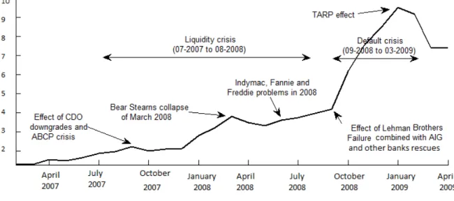
Figure 1 reports the evolution of credit spreads from January 2007 to April 2009. It also indicates the main developments associated with the financial crisis during that period.17 We note the three periods of the financial crisis identified by Saunders and Allen (2010): 1) Mortgage market crises before 07-2007; 2) Liquidity crisis (07-2007 to 08 2008); and 3) Default crisis (09-2008 to 03-2009).
We observe two important jumps in credit spreads dynamics during the financial crisis period that are associated with the periods of liquidity and default crises (07-2007 to 03-2009). The first jump starts during the Fall of 2007 and is associated with the freeze of ABCPs and the CDO downgrades. In March 2008, the bank Bear Stearns experienced difficulties and Lehman Brothers failed in September 2008, which corresponds to the starting date of the second jump. AIG was rescued in the same period, as were other banks. The corporate bond spreads continued to increase until the end of 2008, when the Federal Reserve started to inject liquidity in the market. In the reminder of the paper we will identify the financial crisis as the sub-period from 07-2007 to 03-2009 to concentrate on liquidity and default crises.
[Insert Figure 1 about here]
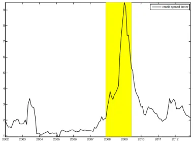
The recession during 2001 (03-2001 to 11-2001) generated a long recovery period in the industrial market after the end of that recession. Many high technological firms had great difficulties recovering their previous growth. This is why corporate credit spreads were still high during 2002 and 2003, representing a strong persistence period in credit risk (see Figure 2). In fact, corporate credit spreads were higher during the period following the 2001 recession than during the recession itself (see Maalaoui Chun et al, (2013) for more details). Then, credit spreads were low until the middle of 2007, and began to increase sharply in the second period of the financial crisis identified as the liquidity crisis (07-2007 to 08-2008) by Saunders and Allen (2010). It seems that the 2006-2007 credit crisis in the mortgage market before the liquidity crisis of 2007-2008 had little impact on the corporate bond market and that the 2005 increase in interest rates had not effect on corporate bond spreads.
17
A similar figure is illustrated in Saunders and Allen (2010), yet they use the Kansas City of Financial Distress Index which looks very similar to our bond spread measure.
Panel B of Figure 2 presents the evolution in the time series of credit spreads around the 2007-2009 financial crisis period while Panel A presents the same time series around the NBER recession. Again, we observe two important jumps in credit spreads during the liquidity and default crisis periods. The first one precedes the start of the NBER recession from 12-2007 to 06-2009 and the second one is during the recession. It seems that that credit risk had predictive power on the recession. Is this due to default risk or liquidity risk in the banking system? We shall answer this question later. Finally, there is another important per-sistence effect after the 2009 economic recession, and our regime shift detection model should be able to separate the default risk effect from the liquidity risk effect in this persistence.
[Insert Figure 2 about here]
V.2 Credit risk regimes
For our regime detection, we use an initial cut-off length of six data points (m = 6), and a Huber parameter of two (h = 2) which controls for outliers in credit spreads series. We also prewhitened the data before applying the regime detection technique to reduce the possibility of detecting false regimes. All the detected regimes are significant at least at the 95% confi-dence level ( = 0:05). Shift points for credit spreads are reported in Table 1, Panel A and can be summarized as follows.
[Insert Table 1 about here]
A first positive shift is detected in Septemebr 2007, three months before the official start of the NBER recession and two months following the official starting date of the financial crisis. The level of credit spreads increased from 1.60% to 3.66%. A second shift occured in October 2008 increasing the level to 7.95%. This second shift seems to reflect the starting official date of the default crisis in September 2008. The two positive credit spread regimes last for 13 months (first regime) and seven months (second regime). In May 2009, we detect a first negative regime. The level of credit spreads decreased from 7.95% to 4.40% but considered still high relative to its level before the crisis period (1.60%). This first negative shift came two months after the official end of the default crisis in March 2009. A second negative shift occured in January 2010 and the level of credit spreads is reduced to 2.48%, again still higher than the initial level of 1.60%.
Our results are consistent with two important aspects of the credit spreads documented in the literature: the predictive aspect and the persistence aspect of credit spreads toward recessions. As noted earlier, the increase in the level of credit spreads preceeded the recession, and the high level regime persisted long time after the recession (Figure 3, Panel A) and the financial crisis period (Figure 3, Panel B). To understand the origins of these two aspects in the data, we break down these credit risk shifts into default and liquidity regime shifts. This allows us to obtain a more detailed interpretation of the driving forces of both crises.
[Insert Figure 3 about here]
V.3 Statistics and detection of default risk regimes
Table 2 reports summary statistics for the daily CDS premiums of different maturities (6 months to 10 years), the recovery rates (1 wi), and the corresponding credit spreads (CS).
[Insert Table 2 about here]
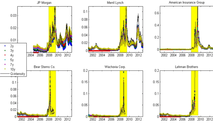
Figure 4 presents the CDS premiums of bonds issued by different investment banks and AIG around the NBER recession. The series of Lehman Brothers ends with its bankruptcy date, and those of Bear Stearns and Wachovia end with their acquisition dates by J.P. Morgan and Wells Fargo respectively. Merrill Lynch continues to operate under its original name even if it merged with Bank of America, and AIG still operates under its original name after being bailed out by the US government in September 2008. It is interesting to observe that even if all spreads increased significantly during the recession, none moved significantly before the recession. The liquidity risk crisis period identified by Saunders and Allen (2010) therefore does not seem to have affected these default premiums significantly. The variation in premi-ums may be related to the default risk of these institutions, and their relative value seems to support that observation. It is interesting to observe that the premiums of JP Morgan are much lower than those of the other institutions, and those of AIG were particularly high at the end of the recession period even after it was rescued by the US Government.
[Insert Figure 4 about here]
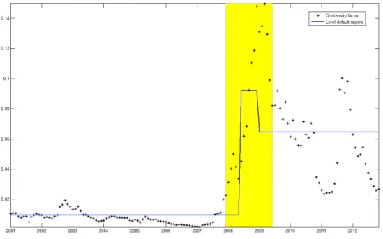
We illustrate the dynamics of the default risk factor from January 2001 to December 2012 in Figure 5. We plot the default factor obtained as an average of the Q-intensity of default obtained from our CDS data of all the firms in our sample for which CDS products were sold (129 firms including the six institutions in Figure 4). The shaded regions represent the NBER recession period (12-2007 to 06-2009) in Panel A and the financial crisis period (07-2007 to 03-2009) in Panel B. We obtained the Q-intensity for each firm by fitting the CDS data for different maturities (six months to ten years for each issuer in the dataset) into the LMN setting. For our regime detection, we use an initial cut-off length of six data points (m = 6) and a Huber parameter of two (h = 2) after prewhitening the data on the default factor. All the detected regimes are significant at least at the 95% confidence level ( = 0:05).
Both the statistics of the Q-intensity factor and the level default regime clearly indicate that default risk was not important before June 2008. Interestingly, the first positive shift we detect is in June 2008 as shown in Table 1, Panel B. The default risk increased from 0.01% to 0.09%. This high default risk regime lasts for seven months. A second shift is detected thereafter in January 2009. Although the shift is negative lowering the default risk from 0.09% to 0.06%, it is still considered very high relative to the initial level of 0.01% before
the crisis. The second high level regime lasts for 48 months. Therefore, the default risk exhibits a persistent pattern towards the NBER recession. This persistence in the default risk is consistent with the theoretical results of recent literature on dynamic structural models (Hackbarth, Miao, and Morellec, 2006; Chen, 2010; and Bhamra, Kuehn, and Strebulaev, 2010). The same persistence is also documented in monetary and credit supply effects models of Bhamra, Fisher and Kuehn (2011), Bernanke and Gertler (1989), King(1994), and Kiyotaki and Moore (1997).
[Insert Figure 5 about here]
V.4 Statistics and detection of liquidity risk regimes
Table 3 reports the summary statistics of the eight liquidity measures considered in this study: Amihud, IRC, Amihud Risk, IRC Risk, Roll, Turnover, Bond Zero trade, and Firm Zero trade. Table 4 reports the correlation coefficients between these measures. Noticebly, the higher correlations are between the Roll measure and the IRC (0.77) and IRC risk (0.73) measures. The correlations between the Amihud and Amihud Risk measures with the Roll measure and with IRC and IRC Risk measures are low.
[Insert Table 3 and 4 about here]
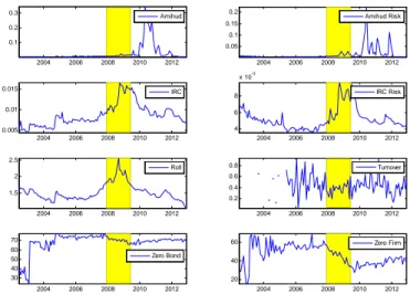
Figure 6 presents the evolution of our eight illiquidity measures during the 2002-2012 pe-riod along with the NBER recession (Panel A) and the financial crisis (Panel B) pepe-riods. The most important observed jumps are for Amihud, IRC and Roll measures of illiquidity. These measures combine information on transaction volumes and bid-ask spreads in the bond mar-ket during these periods. The volatility measures of IRC and Amihud risk are also sensitive to the financial crisis and recession periods. It is interesting to observe a disctinct pattern in the different liquidity measures. The IRC and IRC volatility exhibit two important jumps around the crisis periods –one before the NBER recession and one in the middle of the reces-sion. These jumps capture the increase in bond transaction costs and the start of the liquidity shortage episode. Interestingly, the Amihud and Amihud Risk jumps are observed outside of both the NBER recessionary period and the financial crisis period. These Amihud jumps are likely to reflect a different episode of high liquidity distress after the official crisis periods.
[Insert Figure 6 about here]
Results of the principal component analysis of the illiquidity variables are shown in Ta-ble 5. Panel A presents the eigenvalues of the eight principal components corresponding to the eight illiquidity indicators presented in Section III.2. Panel B shows their corresponding eigenvectors. Results indicate that the first principal component explains 42% of total de-pendence. This first component includes the IRC measure, the IRC Risk measure, and the Roll measure, consistent with the correlation matrix in Table 4. We use the results of this
first principal component to construct our measure for the liquidity factor. Specifically, the liquidity factor is obtained as the average of the IRC, the IRC risk, and the Roll measures.
[Insert Table 5 about here]
As for the default factor, we apply the regime detection technique to the liquidity factor. We also use an initial cut-off length of six data points (m = 6) and a Huber parameter of two (h = 2) after prewhitening the data on the liquidity factor. Results of the liquidity regime are illustrated in Figure 7. The plot spans from July 2002 to December 2012. The shaded region represents the NBER recession period in Panel A and the financial crisis period in Panel B. All the detected regimes are significant at least at the 95% confidence level ( = 0:05). We report the detected shift points in Table 1, Panel C.
[Insert Figure 7 about here]
The first positive shift in the liquidity factor is detected in July 2007 at the beginning of the financial crisis (July 2007) and few months before the beginning of the NBER recession (December 2007). This first positive shift reflects the beginning of a regime of high level of liquidity risk. A second positive shift is detected in June 2008 and the liquidity risk increased from 0.61% to 0.73% as measured by our liquidity factor. These two high regimes of liquidity distress last for 61 months (first regime) and 11 months (second regime). Interestingly, we also detect a first negative regime in Mars 2009, the official end date of the financial crisis (Saunders and Allen, 2010), yet few months before the NBER official end date (June 2009). The first negative shift reduced the level of liquidity risk from a high level of 0.73% to another high level of 0.52%. Thus the bond market was in a high liquidity distress regime both during the entire periods of NBER recession and financial crisis and also about two more years (19 months) after these periods. The high liquidity risk regime ended with the shift detected in February 2012, more than two years after the Federal Reserve intervention. After this second negative shift the liquidity risk factor returned to its level before the crisis (0.42% in 2012 compared to 0.47% in 2002).
To sum up, our results confirm that the financial crisis started with a liquidity shortage but this shortage was amplified in the middle of the financial crisis. Our results partially support the decomposition of the financial crisis between a liquidity risk period from July 2007 to August 2008 and a default risk period from September 2008 to March 2009. Specifically, our results suggest that the liquidity period starts from July 2007 but ends in February 2012 following the second negative shift in the level of the liquidity risk factor. The default risk period detected by the regime shift model lasts from June 2008 to January 2009, a period that is very close to Saunders and Allen’s (2010) default period. Finally, we notice that the liquidity risk crisis preceded the NBER recession period while the default crisis period started after the beginning of the NBER recession period. Therefore, we conclude that the predictive aspect of credit spreads on the 2009 NBER recession stems from the liquidity risk instead of default risk.
I
VI. Conclusion
This paper analyzes credit risk regimes in the corporate bond market during the period 2002-2012 that includes the last financial crisis and the last NBER recession. Our goal is to explain the sources of corporate bond regime shifts by analyzing two of their components in detail: default and liquidity regime shifts.
By superimposing credit regimes on liquidity regimes and default regimes, we link, con-trast and discuss the most important credit-related cycles in the bond market and study their behavior at the onset of economic recessions. Our analysis highlights the nature of the credit regime component, which serves as a forward-looking measure of financial and economic downturns. Specifically, we document the question of whether it is possible to attribute this characteristic of credit spreads to predict economic recessions to a shift in the liquidity risk or a shift in the default risk of the bond market. Our results offer new insights into developing dynamic structural equilibrium models for credit risk as well as for modeling the empirical dynamics of the credit risk premium. To our knowledge, no previous work has directly linked the credit regime to both default and liquidity regimes.
Our results show that two liquidity risk shifts occurred during the financial crisis period of 07-2007 to 03-2009: one at the beginning of the financial crisis period (07-2007) and a second more important one occurred in the middle of the crisis period (06-2008). This means that the first liquidity regime shift occurred before the NBER recession (12-2007 to 06-2009). This first liquidity regime shift seems to explain the predictive power of credit risk on the 2007-2009 NBER recession.
Regarding the default risk regimes, an important regime shift occurred in June 2008, well after the beginning of both the financial crisis and NBER recession starting dates. Yet the persistence effect of the default risk factor after both periods seems much stronger than the persistence effect of the liquidity risk factor, which is consistent with the recent theoretical literature on dynamics structural default risk models.
These preliminary results are very encouraging. They indicate that our new regime shift detection methodology adequately captures the shifts in credit, default and liquidity risks. They also show that rating and pricing models of corporate bonds must integrate a liquidity factor in their analysis, and not only a default factor. Finally they confirm the objective of Basel III to include liquidity risk in the computation of regulatory capital
Many extensions of our analysis are worth doing. We consider four of them here. First, it would be interesting to know the proportions of default risk and liquidity risks in the to-tal yield spread. The recent paper by Dick-Nielse, Feldhütter and Lando (2012) shows that liquidity risk may have represented up to 40% of the credit spread before and after the sub-prime crisis (2005-2009). Although they controlled for default risk in their analysis, they did not explicitly analyze the proportion of default risk in the total credit spread.
Second, it would be interesting to separate the CDSs sold by the institutions in financial difficulty from other sellers to see how the CDS premium is explained not only by the default
risk of the bond issuer but also by the default risk of the protection seller. It would also be important to verify if the CDS premiums contain liquidity risk. Finally, our model does not consider systemic risk. Recently, Allen et al (2012) showed that aggregate systemic risk exposure of the banking sector can predict microeconomic downturns. Extending our regime shift detection model to dependent risks would represent a major extension of our approach.
VII. Appendix: Estimation details of the default model
Following Longstaff, Mithal, and Neis (2005), the default time i follows a CIR process with
intensity i t: d it= i i it dt + i q i tdZti: (18)
Then , the value of the premium leg can be expressed as follows:
P (si; T ) = si tn X ti=1 E e R0tirsds E e R0ti i tds ; (19) = si tn X ti=1 D(ti)E e Rti 0 itds ; = si tn X ti=1 D (ti) Ai(ti) eBi(ti) i 0;
and, the value of the protection leg can be expressed as follows:
P (wi; T ) = E e R i 0 rsds1 f i tngwi ; (20) = wi Z tn 0 E e R0irsds E te Rt 0 sds dt = wi Z tn 0 D(ti)E te Rt 0 sds dt; = wi Z tn 0 D (ti) Gi(ti) + Hi(ti) i0 eBi(t) i 0dt;
where D (ti) is the discount factor, (1 wi) is the recovery on the reference entity per unit
parameters ( ; ; ) : A (t) = e ( + ) 2 t 1 1 e t 2 2 ; (21) B (t) = 2 + 2 2 (1 e t); G (t) = e t 1 e ( + )2 t 1 1 e t 2 2+1 ; H (t) = e ( + )+ 2 2 t 1 1 e t 2 2+2 ; and = q 2 2+ 2; = + : (22)
Note that H (t) = A (t) B0(t) and G (t) = A0(t).
References
[1] Acharya, Viral (2013) ’Understanding Financial Crises: Theory and Evidence from the Crisis of 2007-8.’ NBER Reporter 1
[2] Acharya, Viral, Philipp Schnabl, and Gustavo Suarez (2013) ’Securitization without Risk Transfer,’ Journal of Financial Economics 107, 515-536
[3] Acharya, Viral, Yakov Amihud, and Sreedhar T. Bharath (2012) ’Liquidity Risk of Corpo-rate Bond Returns: A Conditional Approach.’ Journal of Financial Economics, forthcom-ing. Available at SSRN: http://papers.ssrn.com/sol3/papers.cfm?abstract_id=1612287
[4] Allen, Jason, Ali Hortaçsu, and Jakub Kastl (2011) ’Analyzing Default Risk and Liquidity Demand during a Financial Crisis: The Case of Canada.’ Working Paper 2011-17, Bank of Canada
[5] Allen, Linda, Turan G. Bali, and Yi Tang (2012) ’Does Systemic Risk in the Financial Sector Predict Future Economic Downturns?’ Review of Financial Studies 25, 3000-3036
[6] Amihud, Yakov (2002) ’Illiquidity and Stock Returns: Cross-Section and Time-Series Effects.’ Journal of Financial Markets 5 , 31-56
[7] Bai, Jushan (2010) ’Common Breaks in Means and Variances for Panel Data.’ Journal of Econometrics 157, 78-92
[8] Bai, Jushan, and Pierre Perron (1998) ’Estimating and Testing Linear Models with Mul-tiple Structural Changes.’ Econometrica 66, 47-78
[9] Bai, Jushan, and Pierre Perron (2003) ’Computation and Analysis of Multiple Structural Change Models.’ Journal of Applied Econometrics 18, 1-22
[10] Basle III (2010) ’Basel III: ’A Global Regulatory Framework for More Resilient Banks and Banking Systems,’ Bank for International Settlements Working Series.
[11] Beaupain, Renaud, and Alain Durré ( 2013) ’Central Bank Reserves and Interbank Mar-ket Liquidity in the Euro Area.’ Journal of Financial Intermediation 22, 259-284
[12] Bernanke, Ben S. (2013) The Federal Reserve and the Financial Crisis - Lectures. Prince-ton University Press
[13] Bernanke, Ben S., and Mark Gertler (1989) ’Agency Costs, Net Worth, and Business Fluctuations.’ American Economic Review 79, 14-31
[14] Bhamra, Harjoat S., Adlai J. Fisher, Lars-Alexander Kühn (2011) ’Monetary Policy and Corporate Default.’ Journal of Monetary Economics 58, 480-494
[15] Bhamra, Harjoat S., Lars-Alexander Kühn., and Ilya A. Strebulaev (2010) ’The Levered Equity Risk Premium and Credit Spreads: A Unified Framework.’ Review of Financial Studies 23, 645-703
[16] Buraschi, Andrea, Fabio Trojani, and Andrea Vedolin (2011) ’Economic Uncertainty, Dis-agreement, and Credit Markets.’ Working paper, London School of Economics
[17] Cenesizoglu, Tolga, Badye Essid (2012) ’The Effect of Monetary Policy on Credit Spreads.’ Journal of Financial Research 35, 581-613
[18] Chant, John F. (2013) ’Is the Regulation of Financial Institutions Meeting Its Public Policy Objectives?’ Mimeo
[19] Chant, John F. (2008) ’The ABCP Crisis in Canada: The Implications for the Regulation of Financial Markets.’ Canada Expert Panel on Securities Regula-tion: http://www.expertpanel.ca/eng/reports/research-studies/the-abcp-crisis-in-canada-chant.html
[20] Chen, Gongmeng, Yoon K. Choi, and Yong Zhou (2005) ’Nonparametric Estimation of Structural Change Points in Volatility Models for Time Series.’ Journal of Econometrics 126, 79-114
[21] Chen, Hui (2010) ’Macroeconomic Conditions and the Puzzles of Credit Spreads and Cap-ital Structure.’ Journal of Finance 65, 2171-2212
[22] Chen, Nai-Fu (1991) ’Financial Investment Opportunities and the Macroeconomy.’ Jour-nal of Finance 46, 529-554
[23] Chen, Long, Pierre Collin-Dufresne, and Robert S. Goldstein (2009) ’On the Relation between the Credit Spread Puzzle and the Equity Premium Puzzle.’ Review of Financial Studies 22, 3367-3409
[24] Chen, Long, David A. Lesmond, and Jason Wei (2007) ’Corporate Yield Spreads and Bond Liquidity.’ Journal of Finance 62, 119-149
[25] Chen, Ren-Raw, Xiaolin Cheng, and Liuren Wu (2011) ’Dynamic Interactions Between Interest-Rate and Credit Risk: Theory and Evidence on the Credit Default Swap Term Structure,’ Review of Finance, Advance Access Publication, 1-39
[26] Chiaramonte, Laura, and Barbara Casu (2012) ’The Determinants of Bank CDS Spreads: Evidence from the Financial Crisis.’ European Journal of Finance, DOI: 10.1080/1351847X.2011.636832
[27] Chib, Siddhartha (1998) ’Estimation and Comparison of Multiple Change Point Models.’ Journal of Econometrics 86, 221-241
[28] Chun, Albert Lee, and Fan Yu (2013) ’Monolines and the Municipal Bond Market.’ Work-ing Paper, Claremont McKenna College
[29] Collin-Dufresne, Pierre, Robert S. Goldstein, and J. Spencer Martin (2001) ’The Deter-minants of Credit Spread Changes.’ Journal of Finance 56, 2177-2208
[30] Cox, John C., Jonathan E. Ingersoll, and Stephen A. Ross, (1985) ’A Theory of the Term Structure of Interest Rates.’ Econometrica 53, 385–407
[31] Davis, Richard A., Thomas C.M. Lee, and Gabriel A. Rodriguez-Yam (2008) ’Break De-tection for a Class of Nonlinear Time-Series Models.’ Journal of Time Series Analysis 29, 834-867
[32] Degryse, Hans, Frank de Jong, Maarten van Ravenswaaij, and Gunther Wuyts (2005) ’Agressive Orders and the Resiliency of a Limit Order Market.’ Review of Finance 9, 201-242
[33] Dick-Nielsen, Jens (2009) ’Liquidity Biases in TRACE.’ Journal of Fixed Income 19, 43-55
[34] Dick-Nielsen, Jens, Peter Feldhütter, and David Lando (2012) ’Corporate Bond Liquidity Before and After the Onset of the Subprime Crisis.’ Journal of Financial Economics 103, 471-492
[35] Dionne, Georges (2013) ’Risk Management: History, Definition and Critique.’ Risk Management and Insurance Review, forthcoming. Available at SSRN: http://papers.ssrn.com/sol3/papers.cfm?abstract_id=2231635
[36] Dionne, Georges, Geneviève Gauthier, Khemais Hammami, Mathieu Maurice, and Jean-Guy Simonato (2011) ’A Reduced Form Model of Default Spreads with Markov-Switching Macroeconomic Factors.’ Journal of Banking and Finance 35, 1984-2000
[37] Dionne, Georges, Khemais Hammami, Geneviève Gauthier, Mathieu Maurice, and Jean-Guy Simonato (2010) ’Default Risk in Corporate Yield Spreads.’ Financial Management 39, 707-731
[38] Driessen, Joost (2005) ’Is Default Event Risk Priced in Corporate Bonds?’ Review of Financial Studies 18, 165-195
[39] Duan, Jin-Chuan, and Jean-Guy Simonato (1998) ’Estimating and Testing Exponential Affine Term Structure Models by Kalman Filters, Review of Quantitative Finance and Accounting 13, 111-135
[40] Duffee, Gregory R. (1998) ’The Relation between Treasury Yields and Corporate Bond Yield Spreads.’ Journal of Finance 53, 2225-2241
[41] Duffie, Darrell, and Kenneth J. Singleton (1999) ’Modeling Term Structures of Default-able Bonds.’ Review of Financial Studies 12, 687-720.
[42] Duffie, Darrell, and Kenneth J. Singleton (2003) Credit Risk - Pricing, Measurement, and Management. Princeton Series in Finance