HAL Id: hal-02328554
https://hal.archives-ouvertes.fr/hal-02328554
Submitted on 14 Dec 2020
HAL is a multi-disciplinary open access
archive for the deposit and dissemination of
sci-entific research documents, whether they are
pub-lished or not. The documents may come from
teaching and research institutions in France or
abroad, or from public or private research centers.
L’archive ouverte pluridisciplinaire HAL, est
destinée au dépôt et à la diffusion de documents
scientifiques de niveau recherche, publiés ou non,
émanant des établissements d’enseignement et de
recherche français ou étrangers, des laboratoires
publics ou privés.
Accurate measurement of the longitudinal thermal
conductivity and volumetric heat capacity of single
carbon fibers with the 3ω method
Ketaki Mishra, Bertrand Garnier, Steven Le Corre, Nicolas Boyard
To cite this version:
Ketaki Mishra, Bertrand Garnier, Steven Le Corre, Nicolas Boyard. Accurate measurement of the
longitudinal thermal conductivity and volumetric heat capacity of single carbon fibers with the 3ω
method. Journal of Thermal Analysis and Calorimetry, Springer Verlag, 2019,
�10.1007/s10973-019-08568-z�. �hal-02328554�
1
Accurate measurement of the longitudinal thermal conductivity and volumetric heat capacity of single carbon fibers with the 3ω method
Ketaki Mishra (a) *, Bertrand Garnier (a), Steven Le Corre (a), Nicolas Boyard (a)
a CNRS, LTeN UMR 6607, Université de Nantes, Rue Christian Pauc, 44306 Nantes Cedex 3, France. Corresponding author : ketaki.mishra@univ-nantes.fr, 0240683180
Abstract:
An experimental setup for 3𝜔 method with a constant current source and two differential amplifiers was built to measure the thermal conductivity and the volumetric heat capacity of single polyacrylonitrile (PAN)-based carbon fiber. In complement to a well known analytical thermal model, a numerical one was developed that can check the validity of the analytical one and can also take into account the effect of convective heat loss on the measurements. A detailed sensitivity analysis of the unknown parameters was presented that would finally help in the better design of the setup for 3𝜔 method. The tests were performed under vacuum and atmospheric pressure for chromel wire as a reference sample and under vacuum for two types of polyacrylonitrile-based carbon fiber. Detailed measurements were performed displaying the influence of convective loss and the thermal contact resistance between fiber and copper electrodes on the estimation of thermal properties of carbon fiber.
Keywords: 3𝜔 method; thermal conductivity; carbon fibers; sensitivity analysis; thermal contact resistance.
1. Introduction
In the current engineering scenario, carbon fibers reinforced composites have found a great place in many high-performance industries such as aviation, automotive, textile, etc. With the advances in the material technology, many researchers focused their interest in finding out the effective thermal properties of the composite material at different scales starting from macro to micro. Although a lot of research work can be found at macroscale [1][2][3], less studies were dedicated to the estimation of thermal properties at microscale such as at the level of single fiber.
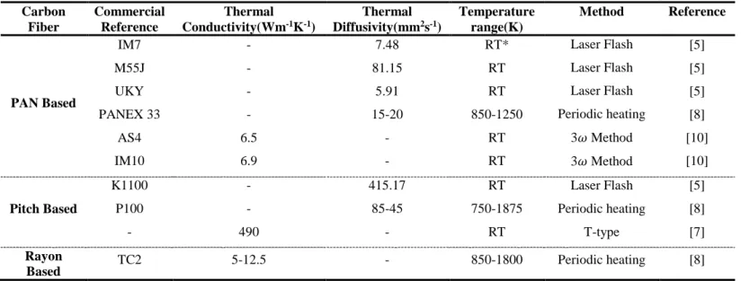
In the literature, some methods use a bundle of fibers to approximate the thermal properties of single fiber such as Angström method or Thermal potentiometer [4] or Laser flash method [5]. There are also a few techniques that work directly on single fibers such as AC calorimetry [6], T-type probe method [7], pulse laser-assisted thermal relaxation technique [8]. A brief detail of these techniques is presented in Table1. Some thermal conductivity values measured using these techniques are shown in Table 2 for different types of carbon fibers. These techniques mainly focus on the estimation of single thermal property such as either thermal conductivity or specific heat or thermal diffusivity during one experiment. Contrary to these techniques, the 3𝜔 method is a strong benchmark that has the capability of measuring these thermal properties simultaneously. Furthermore, the applicability of the 3𝜔 method is large, it was used for solids at micro[9] to macro scales[10], liquids and gases[11][12]. Less focus was given in adopting the 3𝜔 method for measuring the thermal properties of single carbon fiber.
This technique consists in heating the sample with an alternating current at a frequency . The current leads to temperature fluctuations at 2𝜔, ultimately resulting in fluctuations of the voltage at both 𝜔 and 3𝜔 as it will be discussed in details further. The variation of the 3𝜔 voltage with the frequency contains the information about the
2
thermal properties such as thermal conductivity and volumetric heat capacity of the sample. It is therefore important to eliminate the 1 𝜔 voltage by certain improvement in the setup such as a Wheatstone bridge [9] or an analog balance bridge circuit [13].
Table 1 Literature survey on different methods used for thermal property measurement of carbon fiber
This not only increases the stability of the 3𝜔 voltage but also increases the accuracy in the estimation of thermal properties [15]. In the literature, there are multiple experimental configurations based on the type of sources such as constant current [13] or constant voltage source [16]. The milestone research work was provided in the paper of Lu [9] where he discussed the simultaneous measurement of the thermal conductivity and volumetric heat capacity of single platinum wire and carbon nanotube bundles acting itself as heater and sensor. This paper provided the basic analytical thermal model that can enable the estimation of thermal properties and many detailed experimental tips while performing the 3𝜔 method experiments under vacuum. It also dealt with radial heat losses due to radiation and convection by choosing proper approximation. None of the previous research showed the sensitivity of the measured voltage with respect to the thermal properties as function of the working frequency range that directly depends on the length of the sample used. The lack of sensitivity could explain the variation of measurement of thermal properties with change in the length for the same sample [13].
This paper is aimed at providing a detailed analysis of the implementation of a 3𝜔 method for carbon fibers, giving design tips for a proper choice of sample dimensions and frequency range and quantifying the precision of the measurements. After presenting the principle and the analytical modeling of the 3𝜔 method [9] applied to the measurement of the thermal properties for wires or fibers, we show a complementary numerical formulation of the heat transfer equation that enables to account for lateral heat losses. On the basis of those tools, a sensitivity analysis of the measured voltage with respect to the thermal conductivity and volumetric heat capacity over a wide frequency range (10-2-104 Hz) is then presented. It highlights the importance of choosing a proper length of the sample with higher sensitivity that can ultimately improve the accuracy of the measurements. This leads to a proper experimental design which is detailed afterwards. Lastly, the thermal conductivity and volumetric heat capacity
Method Heating Method Temperature sensor Sample Type Reference
Angstrom Method Constant DC current
heater (Joule Heating) Thermocouples Fiber Bundle [4]
Laser Flash Method Short Laser Pulse IR sensor Fiber Bundle [5]
Thermal Potentiometer
Constant DC heater
(Joule Heating) Thermocouples Fiber Bundle [4]
AC Calorimetery Halogen Lamp Thermocouple Single Fiber [6]
T-Type Probe Method
Constant DC heater
(Joule Heating) Hot wire Single Fiber [7]
Periodic heating
technique Argon Laser Beam IR sensor Single Fiber
[8]
3𝛚 Method AC power supply heater (Joule Heating)
Sample dependent.
3
are measured for a chromel wire and two types of PAN-based carbon fibers and the effect of thermal contact resistance between sample and its holder is discussed.
Table 2 Longitudinal thermal conductivity and thermal diffusivity values of carbon fiber from literature.
(*RT= Room temperature)
2. Analytical Model
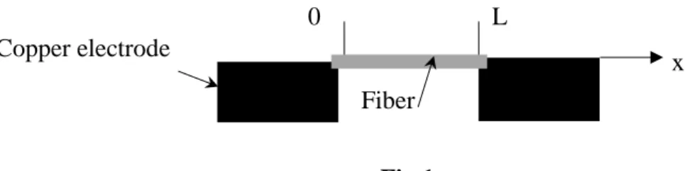
The schematic diagram of the sample over the copper electrodes is depicted in Fig. 1. The fiber, assumed straight and of length L, is connected to two electrodes of constant temperature and submitted to an alternating current with a given frequency. The measurement of the voltage between the two electrodes over a certain range of frequencies is then used to identify the thermal properties, by using a thermal model, which can be either analytical or numerical.
This section provides a brief introduction of the analytical model for the 3𝜔 voltage response of a self-heating fiber depending on the imposed frequency (𝜔). The model assumes that the specimen is a uniform cylinder placed between two heat sinks (copper electrode) with perfect contact at the joints (Fig. 1). An alternating electrical current (𝐼0𝑠𝑖𝑛 (𝜔𝑡)) with a frequency 𝜔 passed through the sample that has an electrical resistance 𝑅 and length 𝐿.
Fig 1 Schematic diagram of the fiber sample with copper holders
Lu [9] has developed an analytical model for 1D heat conduction with a source term along the fiber that can predict the 3𝜔 voltage through the sample. The partial differential equation for solving the corresponding heat conduction problem is as follows:
𝜌𝐶𝑝 𝜕 𝜕𝑡𝑇(𝑥, 𝑡) − 𝑘 𝜕2 𝜕𝑥2𝑇(𝑥, 𝑡) = 𝐼02𝑠𝑖𝑛2𝜔𝑡 [𝑅0(1 + 𝛼𝑒(𝑇(𝑥, 𝑡) − 𝑇0)] (1)
with the following boundary and initial conditions:
{
𝑇(0, 𝑡) = 𝑇0
𝑇(𝐿, 𝑡) = 𝑇0
𝑇(𝑥, 0) = 𝑇0
(2)
where 𝜌 is the density, 𝐶𝑝 is the heat capacity, 𝑘 is the thermal conductivity, 𝜔(2𝜋𝑓) is the angular frequency, 𝑓
is the frequency, 𝑇 is the temperature of the sample at position x and time t, 𝑇0 is the ambient temperature, 𝐼0is
Carbon Fiber Commercial Reference Thermal Conductivity(Wm-1K-1) Thermal Diffusivity(mm2s-1) Temperature range(K) Method Reference PAN Based IM7 M55J UKY PANEX 33 AS4 IM10 - - - - 6.5 6.9 7.48 81.15 5.91 15-20 - - RT* RT RT 850-1250 RT RT Laser Flash Laser Flash Laser Flash Periodic heating 3𝜔 Method 3𝜔 Method [5] [5] [5] [8] [10] [10] Pitch Based K1100 P100 - - - 490 415.17 85-45 - RT 750-1875 RT Laser Flash Periodic heating T-type [5] [8] [7] Rayon
4
the amplitude of the current, 𝑅0 is the electrical resistance of the fiber at 𝑇0, 𝛼𝑒 is the temperature coefficient of
this electrical resistance. By applying impulse theorem the temperature distribution through the sample can be derived as [9]: 𝑇(𝑥, 𝑡) − 𝑇0= ∆0∑ [1 − (−1)𝑛] 2𝑛3 ∗ 𝑠𝑖𝑛 ( 𝑛𝜋𝑥 𝐿 ) [1 − ( 𝑠𝑖𝑛(2𝜔𝑡 + 𝜙𝑛) √1 + 𝑐𝑜𝑡2𝜙 𝑛 )] ∞ 𝑛=1 (3) where 𝑐𝑜𝑡𝜙𝑛=2𝜔𝛾𝑛2, 𝛾 = 𝜌𝐶𝑝𝐿2
𝜋2 𝑘 is the thermal time constant for axial thermal transfer and 𝛥0=2𝐼0
2𝑅𝐿
𝜋𝑘𝑆 is the
maximum DC temperature accumulation at the center of the specimen. Eq. 3 is obtained under the following condition that enables the proposed truncation Eq.3 of the solution.
𝛿0=
𝐼02𝑅′𝐿
𝑛2𝜋2𝑘𝑆≪ 1
(4)
where 𝑅′= 𝑅
0𝛼𝑒 and S is the cross sectional area. The temperature fluctuating at a frequency of 2𝜔 gives rise to
a resistance fluctuation at the same frequency and can be expressed as: 𝛿𝑅 = 𝑅′∆0∑ [1 − (−1)𝑛]2 2𝜋𝑛4 [1 − ( 𝑠𝑖𝑛(2𝜔𝑡 + 𝜙𝑛) √1 + 𝑐𝑜𝑡2𝜙 𝑛 )] ∞ 𝑛=1 (5)
where 𝜙𝑛 is the value of the phase constant. The expression of resistance fluctuation can then be added to the
initial resistance 𝑅0 of the sample to obtain the total resistance(𝑅0+ 𝛿𝑅). This value of total resistance is then
multiplied with the applied alternating current 𝐼0𝑠𝑖𝑛(𝜔𝑡) to obtain the voltage drop across the sample,
𝑉 = 𝐼𝑅 = 𝐼(𝑅0+ 𝛿𝑅) = 𝑓(𝜔) + 𝑔(3𝜔) (6)
The voltage has two components, one depending on frequency 𝜔 and the other one on 3𝜔 . The 3𝜔 part contains the information about the thermal properties as it is the fluctuating temperature dependent part of the overall voltage drop. The average (Root Mean Square) voltage at 3𝜔 frequency can be written as follows [9]:
𝑉3𝜔 𝑟𝑚𝑠≈ − 4𝐼𝑟𝑚𝑠 3 𝐿𝑅𝑅′
𝜋4𝑘𝑆√1 + (2𝜔𝛾)2
(7)
The RMS values of voltage at frequency 3𝜔 (𝑉3𝜔 𝑟𝑚𝑠) is therefore a function of frequency and other parameters
that are constants to be measured beforehand. Thus fitting this model with the experimental results enables to estimate the unknown parameters which are thermal conductivity and volumetric heat capacity of the sample under study. Successful implementation of this model obviously requires an accurate measurement of all the parameters governing Eq. 7 such as RMS current (𝐼𝑟𝑚𝑠), length (𝐿), temperature coefficient of resistance (𝛼𝑒), cross sectional
surface area of the sample (S).
In the same work [9], the condition for neglecting the heat losses due to radiation is also given. It states that conductive power should be much higher than the power dissipated due to radiation.
𝛿1=
16𝜖𝜎𝑇03𝐿2
𝜋2𝑘𝐷 ≪ 1
(8)
where 𝜖 is the fiber emissivity and 𝜎 the Stefan Boltzmann constant and D is the diameter of the sample under study.
5
3. Numerical modelPrevious researches on 3𝜔 method were restrictive to experiments in a vacuum chamber. This motivated the development of a numerical model that could not only work under vacuum but also approximate the effect of convective losses. This section shows a brief description of the numerical model for estimating the 3𝜔 response of one fiber in the configuration depicted in Fig. 1 after passing an alternating current. In the case of constant thermophysical parameters, the heat transfer phenomena can be described by the following 1D partial differential equation: ∑ 𝑐 ∞ 𝑛=1 𝜌𝐶𝑝 𝑘 𝜕 𝜕𝑡𝑇(𝑥, 𝑡) − 𝜕2 𝜕𝑥2𝑇(𝑥, 𝑡) + 𝑚2(𝑇(𝑥, 𝑡) − 𝑇𝑜) = 𝑄 𝑘 (9)
where 𝑚2= 4ℎ 𝑘𝐷⁄ with h the heat transfer coefficient of air that surrounds the sample. Q is the average volumetric heat source due to the alternating current. By choosing ∆𝑇(𝑥, 𝑡) = 𝑇(𝑥, 𝑡) − 𝑇𝑜 , the above equation
can be transformed to ∑ 𝑐 ∞ 𝑛=1 𝜌𝐶𝑝 𝑘 𝜕 𝜕𝑡∆𝑇(𝑥, 𝑡) − 𝜕2 𝜕𝑥2∆𝑇(𝑥, 𝑡) + 𝑚2(∆𝑇(𝑥, 𝑡)) = 𝑄 𝑘 (10)
Implementing one of the deductions from the analytical model that the temperature is fluctuating at 2𝜔 frequency and so as the volumetric heat source (2𝑅𝐼𝑟𝑚𝑠2
𝑆𝐿
⁄ ~𝑓(2𝜔)), the terms ∆𝑇 and 𝑄 can be sought in the following periodic form:
∆𝑇 = 𝑅𝑒(𝑇̃𝑒𝑗2𝜔𝑡), 𝑄 = 𝑅𝑒(𝑄̃𝑒𝑗2𝜔𝑡) (11)
where 𝑇̃ and 𝑄̃ are the complex expressions of the temperature drop and volumetric power respectively. Re designates the real part of a complex expression. Eq. 10 can be transformed by implementation of Eq. 11 to:
𝜕2𝑇̃ 𝜕𝑥2= − 𝑄̃ 𝑘+ ( 𝑗2𝜔ρC𝑝 𝑘 + 𝑚2) 𝑇̃ (12)
The spatial boundary conditions present in Eq. 2 can be transformed to Eq. 13 { 𝑇̃ = 0, 𝑥 = 0
𝑇̃ = 0, 𝑥 = 𝐿
(13)
A 1D mesh representative of the sample was generated and a central finite difference approach was used to solve the Eq. 12 by implementation of the boundary conditions of Eq. 13 . The discrete matrix representation of the Eq. 12 and 13 is [ 𝑇̃2 𝑇̃3 ⋮ ⋮ ⋮ 𝑇̃𝑁−1] = [ 𝛽 0 … … 0 𝛽 0 … 0 0 𝛽 … 0 ⋮ ⋮ ⋱ ⋱ ⋱ 0 ⋮ ⋮ 0 ⋱ ⋱ ⋱ 0 0 0 0 𝛽] −1 [ ⋮ ⋮ ⋮ ] with { 𝛾 =𝛥𝑥12 = − [𝛥𝑥22+𝑗2𝜔𝜌𝐶𝑝 𝑘 + 𝑚 2] 𝛿 = −𝑄̃𝑘 (14)
6
The complex form of the temperature rise at all nodes (𝑇̃2, 𝑇̃3… 𝑇̃𝑁−1) can be estimated by solving this linear
system. The modulus of the average of this temperature rises over all nodes (N) gives the average longitudinal temperature rise 𝑇𝑎𝑣 of the sample:
𝑇𝑎𝑣= ‖∑ 𝑇̃𝑖 𝑁
1
‖ /𝑁 (15)
The overall voltage response measured in 3𝜔 method is the modular 𝑉3𝜔 𝑟𝑚𝑠 of the sample and thus the numerical
𝑉3𝜔 𝑟𝑚𝑠 can be expressed as follows:
𝑉𝑟𝑚𝑠= 𝐼𝑟𝑚𝑠(𝑅0+ 𝑅0𝛼𝑒𝑇𝑎𝑣) = 𝑓(𝜔) + 𝑔(3𝜔) (16)
𝑉3𝜔 𝑟𝑚𝑠 = 𝐼𝑟𝑚𝑠𝑅0𝛼𝑒𝑇𝑎𝑣 (17)
This step is repeated for estimating 𝑉3𝜔 𝑟𝑚𝑠 for the desired frequencies. The effect of convective loss during the
measurements under atmospheric condition can be approximated by implementation of heat transfer coefficient[17] in the term ‘m’ present in Eq. 14.
4. Comparison between analytical and numerical models
The comparison between analytical and numerical models was proceeded by testing the 3𝜔 voltage fluctuations over a test case for chromel wire (diameter 13 µm) and carbon fiber (diameter 7 µm) , all with a 1.5 mm length. An alternating current of 6mA and 1mA was assumed to pass through the chromel wire and carbon fiber respectively. The values of thermal properties were obtained from the literature or from the wire or fiber suppliers (Table 5 and Table 6). The computed values of 𝑉3𝜔 𝑟𝑚𝑠 under vacuum, by using analytical and numerical
(with h=0) models iare compared in Fig. 2. It showed a good agreement between the 𝑉3𝜔 𝑟𝑚𝑠 values. The difference
lies mostly at lower frequencies (𝑓 < 0.1𝐻𝑧). with a 𝑉3𝜔 𝑟𝑚𝑠 value less than 1.6% of maximum 𝑉3𝜔 𝑟𝑚𝑠. An analogous comparison between the two thermal models was also performed for the case of carbon fiber leading to similar results (discrepancy smaller than 1.6% of the maximum value of 𝑉3𝜔 𝑟𝑚𝑠). Additionally, for each test, the
validity condition of Eq. 4 for the analytical model is well checked with values of 0 as 4×10⁻⁴ for chromel and as
4×10⁻² for carbon fiber.
Fig 2 Numerical and analytical models comparison and effect of convective losses (13.6m chromel wire)
To demonstrate the influence of convective losses, one have chosen an approximate value of heat transfer coefficient using a correlation for natural air convection around a horizontal cylinder [17] with an assumption of max 1K [9] increase in temperature. The radiation losses can be neglected as the criterion of Eq.8 is always respected for the chromel wire (1~0.025) and also carbon fibers (1~0.079). It can be observed from Fig 2 2 that
the convective heat transfer leads to a huge drop of the 𝑉3𝜔 𝑟𝑚𝑠value. Fitting of the analytical model was performed
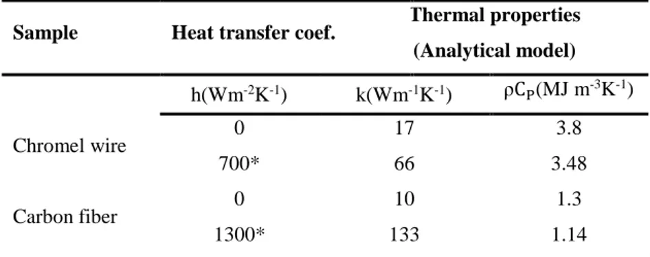
on this case in order to quantify the effect of convective heat loss on the estimation of thermal conductivity and volumetric heat capacity. Table 3 shows that the thermal conductivity value is increased by ~390% and the volumetric heat capacity value is decreased by ~8% for chromel wire if one uses the analytical model which does not take into account heat losses. These biases become more prominent in case of carbon fiber (Table 3) as its thermal conductivity is smaller and also as the approximated heat transfer coefficient almost doubled due to the smaller diameter of carbon fiber. This shows the importance of using vacuum while performing measurements for
7
the estimation of especially thermal conductivity of wire or fibers. For our experimental tests, we have chosen a secondary vacuum with a 10-6 mbar pressure resulting in an air thermal conductivity decrease of four orders of magnitude [18].
Sample Heat transfer coef. Thermal properties
(Analytical model) h(Wm-2K-1) k(Wm-1K-1) ρCP(MJ m-3K-1) Chromel wire 0 17 3.8 700* 66 3.48 Carbon fiber 0 10 1.3 1300* 133 1.14 *: computed using correlation for natural air convection around a horizontal cylinder [17]
Table 3 Thermal conductivity and volumetric heat capacity estimated with and without convective losses
and using the analytical model (Eq.7)
5. Sensitivity Analysis
For the design of new experiments for thermal properties measurement, it is very useful to perform sensitivity analysis of the measured quantities with respect to the unknown parameters. It allows to find the set of experimental conditions that will maximize the sensitivity coefficients and therefore will insure a greater accuracy of the estimated values. In our case, the sensitivity coefficients of the voltage 𝑉3𝜔 𝑟𝑚𝑠 with respect to k and Cp were
studied as function of the frequency and also the sample length.
Fig 3. Sensitivity analysis of the V3 rms voltage to the (a) thermal conductivity and (b) volumetric heat
capacity
As these sensitivity coefficients depend strongly on the sample length, one have considered their reduced expression (𝑋∗ 𝑚) defined as [19]: ∑ 𝑐𝑋∗ 𝑚= 𝑚 𝜕𝑉3𝜔 𝑟𝑚𝑠 𝑚𝑎𝑥 (𝑉3𝜔 𝑟𝑚𝑠)𝜕𝑚, with 𝑚 = 𝑘, 𝜌𝐶𝑝 ∞ 𝑛=1 (18)
The reduced sensitivity coefficients for chromel wire and two types of PAN fibers were computed for sample lengths ranging from 0.5 to 3.5 mm. The thermal conductivity and volumetric heat capacity values were obtained from the literature or from the supplier (Table 5 and Table 6). Fig 33 shows that the sensitivities of voltage 𝑉3𝜔 𝑟𝑚𝑠
with respect to k and Cp are high in a particular frequency range depending on the sample length. Therefore if
one considers a frequency range of 1 to 100 Hz (which provides reasonable measurement duration), the sample length should not exceed too much 1.5 mm.
8
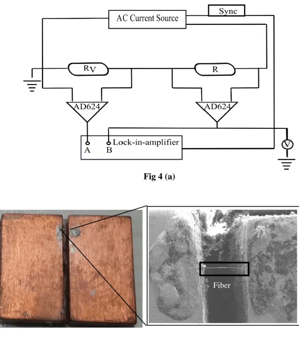
6. Experimental setup and samplesThe constant voltage source based circuit using a Wheatstone bridge has the disadvantage of the measurement of thermal properties for sample of only low electrical resistance, typically less than 400 . As the electrical resistance of carbon fibers are higher (around 500 for a length of 1.5mm), therefore two differential amplifiers (AD624) with a constant current source (Keithley 6221) were used for the detection of the voltage signal in the sample (R) and the variable resistance (RV) as shown in Fig. 4(a). The signal from these two resistances were
fed to the inputs A and B of the Lock in Amplifier (LIA Ametek 7265). The LIA was set to the configuration of A-B, a subtraction mode of the signal from the two AD624. The LIA was first set to 1𝜔 detection mode, which needs to be equal to 0 at each frequency involving RV= R and ultimately led to the cancellation of 1𝜔 signal. The
variable additional resistance was pure resistance with no significant temperature increase. Then the LIA was set to the 3𝜔 detection mode and thus the A-B mode provides the 3𝜔 signal only through the sample.
Fig 4 (a) Electrical setup for 3𝜔 measurement (b) Sample holder (c) Specimen attached to the electrode with silver paste (d) Cross section of the PAN carbon fiber(FT300B) obtained from scanning electron
microscopy
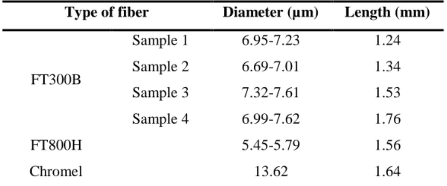
The thermal conductivity and volumetric heat capacity were estimated for the chromel wire and two PAN carbon fibers from Toray Industries, FT300B and FT800H. Single fiber/wire was placed between two copper plates as shown in Fig. 4(b) and (c) and covered carefully with silver paste and given sufficient time for the silver paste to dry Fig. 4 (c). The copper electrodes are acting as both heat sinks and electrical connectors. An accurate measurement of the parameters such as sample length and diameter, involved in the analytical and the numerical model was necessary. A Scanning Electron Microscope and a high-resolution optical camera were used to have an exact measurement of the sample diameter and length respectively. For this paper, the length of each sample was chosen in such a way that the working range frequency is 1-100 Hz thanks to the previous sensitivity analysis, making the 3 measurements quite fast (~30 min for 25 frequency values). Table 4 presents the lengths of the chromel wire and carbon fibers used for performing the 3𝜔 experiments. Later the sample was then placed in a chamber that can work as a secondary vacuum (10−6 mbar) at room temperature. In order to show the influence
of convective heat loss in the parameter estimation by the analytical model, the experiments were also performed at atmospheric pressure (103 mbar) for chromel wire.
Type of fiber Diameter (µm) Length (mm)
FT300B Sample 1 6.95-7.23 1.24 Sample 2 6.69-7.01 1.34 Sample 3 7.32-7.61 1.53 Sample 4 6.99-7.62 1.76 FT800H 5.45-5.79 1.56 Chromel 13.62 1.64
Table 4 Dimension of the samples used for 3𝜔 measurement
Despite the use of instruments with high accuracy, there are few uncertainties on known parameters such as length, diameter, current and etc. The model for the estimation of the overall uncertainty on the thermal conductivity and volumetric heat capacity through transient measurements was presented by Milosevic[20].
9
𝑆𝑓𝑖𝑛𝑎𝑙= [𝑋𝑇 𝑊 𝑋]−1 with 𝑊 = [𝜎𝑉23𝜔 𝑟𝑚𝑠+ ∑ (𝜎𝑚𝑝 𝜕𝑉3𝜔 𝑟𝑚𝑠 𝜕𝑚𝑝 ) 2 𝑝 ] −1 (19)where 𝑋 is the sensitivity coefficient matrix, 𝑊 is the variance covariance matrix, 𝜎𝑉3𝜔 𝑟𝑚𝑠is the variance of
measured 𝑉3𝜔 𝑟𝑚𝑠, 𝜎𝑚𝑝 is the variance of the known parameters p, 𝑆𝑓𝑖𝑛𝑎𝑙 is the matrix of variance and covariance. The values of 𝜎𝑚𝑝 can be estimated with the errors on the known parameters during measurements of 𝑉3𝜔 𝑟𝑚𝑠 for chromel wire represented as 𝑒I=0.1%, eR=0.5%, eαe=0.5%, eD=0.2%, 𝑒L=2.8%. During the measurements for carbon fiber, the error is similar to the chromel except in case of the diameter for which 𝑒𝐷 = 5.1% predicted from
Table 4. The diagonal terms of 𝑆𝑓𝑖𝑛𝑎𝑙 represent the variances m2 of the estimated parameters m (k or Cp) including
the effect of the uncertainty of the known parameters. For a 95% confidence band, the relative uncertainty em on
parameter m is obtained using em=1.96 m/m.
7. Experimental Results
7.1 Chromel wire
The validation of the experimental setup was achieved by choosing a wire with known properties. Therefore a 13.6m diameter chromel wire was tested. Its diameter was checked to be fairly constant with perfectly circular cross-section over the length. Fig. 5 shows the experimental test performed in vacuum and atmospheric condition for a frequency range of 1 to 100 Hz. Both experimental data were fitted by the analytical model to determine the thermal conductivity and volumetric heat capacity of the chromel wire. Table 5 shows the estimated values of the thermal conductivity and volumetric heat capacity for the chromel wire by using 3𝜔 method. The experiments conducted under vacuum showed very good agreement of the measured values for thermal conductivity and volumetric heat capacity with the reference values from the literature. The overall uncertainties in the measurement of thermal conductivity and volumetric heat capacity for chromel are ~2.9% and ~1.3% respectively (section 6). As expected from our initial remark with the influence of convective loss, the thermal conductivity estimated from the experiments performed under the atmospheric condition is very unrealistic and with a discrepancy of ~390% from the reference value [21]. In case of fitting by the numerical model for experiments in an atmospheric condition, the heat transfer coefficient was approximated to be ranging from 450-740 Wm-2K-1 for a temperature rise from 0.1 to 2K and using the correlations presented by Churchill and Chu [17] and also Morgan [25] which are valid for the obtained Rayleigh number during our experiments. The impact of the range of heat transfer coefficient is shown in the estimation of the thermal properties (Table 5) by the numerical model leading the estimated thermal conductivity not reliable under atmospheric condition. In addition, one should note that the used correlations were established for steady state regimes and not periodic ones.
10
Table 5 Thermal properties measured for chromel wire by fitting with the analytical model under vacuum
and atmospheric condition (* this range is due to the range of h value from the correlations [17] and [25] and also due to a 0.1 to 2K temperature rise)
7.2 Carbon fibers
The 3𝜔 method was then used to estimate the thermal properties for the two PAN carbon fibers. Fig. 6(a) shows the experimental 3𝜔 voltage fluctuations with a 1 to 100 Hz frequency range performed in a vacuum chamber. The thermal conductivity and volumetric heat capacity were measured for the four samples of FT300B with different lengths by fitting with the analytical model. Fiber FT800HB was tested for single length of the sample of 1.56 mm (Fig. 6(b)). The measured values of thermal conductivity and volumetric heat capacity for the carbon fibers are presented in Table 6 and compared with the data provided by the fiber supplier (Toray Industries). The uncertainties in the measurement of thermal conductivity and volumetric heat capacity are ~8.1% and ~4.9% respectively for these carbon fibers, as estimated from the uncertainty analysis shown in section 6.
Fig 6 Measured (•) and fitted (‒) V3voltages for (a) FT300B carbon fibers with multiple sample lengths, (b) FT800HB carbon fiber with a 1.56mm sample length
Table 6 Thermal properties estimation for carbon fibers
The experiments performed under atmospheric condition could give an approximate range of thermal property with the condition of proper estimation of theoretical heat transfer coefficient. This is impossible to achieve in case of carbon fiber due to the complex cross section as shown from the SEM image (Fig. 4(d)) and the reliability of the correlation for the estimation of heat transfer coefficient. Although the numerical model could be used for the estimation of heat transfer coefficient along with the thermal conductivity and volumetric heat capacity for an experiment performed under atmospheric condition, but it was observed that the thermal conductivity and heat transfer coefficient are highly correlated parameters, making impossible the correct estimation of these parameters simultaneously.
Thermal Properties Measured Reference[21][22]
Analytical Model Numerical Model
k( Wm-1K-1) Vacuum 18.15 18.27 17.3 Atmospheric 70.15 18.51-25.82 * ρCP( MJ m-3K-1) Vacuum 3.68 3.81 3.85 Atmospheric 3.62 3.81-3.83 * FT300B Reference [23] FT800H Reference [24] Thermal Properties
Sample 1 Sample 2 Sample 3 Sample 4 Supplier datasheet
Supplier datasheet k( Wm-1K-1) 10.11 10.03 10.17 10.28 10.47 34.88 35.13 ρCP( MJ m-3K-1) 1.35 1.38 1.37 1.37 1.39 1.37 1.36
11
7.3 Effect of thermal contact resistance between carbon fiber and copper electrodes
The analytical and numerical model works with an assumption of perfect thermal contact between the sample and copper electrodes, which is impossible to achieve in practice. Therefore an estimation of thermal contact resistance was done from the measured values of thermal conductivity with different lengths of the sample by the calculation of the overall thermal resistance (L/k) for each length. Fig. 7 shows the evolution of thermal resistance with length for the fiber FT300B.
Fig 7 Thermal resistance vs length for FT300B
The measured thermal resistances can be fitted with linear regression. The y intercept of this plot gives the thermal contact resistance when the fiber length is 0. The obtained value (8.83 10-6 m2KW-1 ) can be compared to the intrinsic thermal resistance of the fibers (L/k~10-4 m2KW-1). The overall effect of the thermal contact resistance for the 3𝜔 method is, therefore less than 7% of the thermal resistance (L/k). The inverse of the slope of the linear regression provides the final value of the thermal conductivity of the FT300B carbon fiber which is equal to 10.82 Wm-1K-1.
8. Conclusions
The analytical model for fiber developed by Lu [9] was found to be accurate enough to estimate the thermal conductivity and volumetric heat capacity of small metallic wire and carbon fibers. The importance of experimenting only under vacuum condition was proven by quantifying the influence of convective loss on the estimation of thermal conductivity using this analytical model and a numerical model able to take into account the heat losses. The effect on thermal conductivity is very high, especially for sample of low thermal conductivity. The volumetric heat capacity turned out to be not so affected by convective heat losses. A detailed sensitivity analysis for both thermal conductivity and volumetric heat capacity was done for getting results with higher accuracy. It indeed enabled the choice of an adequate frequency range and sample length. Based on the experimental configuration of differential amplifiers with a constant current source, the results for small chromel wire and carbon fibers obtained under vacuum showed high precision with respect to the reference values. The higher uncertainty in the measurement for carbon fibers is mainly due to the discrepancy of the diameter through the length of samples. The sum of the two thermal contact resistances at both fiber ends was also estimated to be less than 7% of the overall thermal resistance of the sample thus the influence on the measurement of thermal conductivity is small. Finally, the adaptation of the 3𝜔 method to the measurement of the thermal properties of carbon fibers presented here is proved to be efficient and reliable. Furthermore, the uncertainties were thoroughly calculated and provided an acceptable interval of confidence. Further work will be dedicated to the measurement of the radial thermal conductivity of carbon fibers.
Acknowledgements: The authors would like to thanks J. Aubril for the discussions and quality of his technical
12
References1. Sweeting RD, Liu XL. Measurement of thermal conductivity for fibre-reinforced composites. Compos Part A Appl Sci Manuf. 2004;35:933–8.
2. Manocha LM, Warrier A, Manocha S, Sathiyamoorthy D, Banerjee S. Thermophysical properties of densified pitch based carbon/carbon materials-I. Bidirectional composites. Carbon N Y. 2006;44:488–95.
3. Siddiqui MOR, Sun D. Development of Experimental Setup for Measuring the Thermal Conductivity of Textiles. Cloth Text Res J. 2018;36:215–30.
4. Gallego NC, Edie DD, Ntasin LN, Ervin VJ. Modeling the thermal conductivity of carbon fibers. Carbon N Y. 2000;38:1003–10.
5. Craddock JD, Burgess JJ, Edrington SE, Weisenberger MC. Method for Direct Measurement of On-Axis Carbon Fiber Thermal Diffusivity Using the Laser Flash Technique. J Therm Sci Eng Appl [Internet]. 2016;9:014502. 6. Yamane T, Katayama SI, Todoki M, Hatta I. Thermal diffusivity measurement of single fibers by an ac calorimetric method. J Appl Phys. 1996;80:4358–65.
7. Wang JL, Gu M, Zhang X, Song Y. Thermal conductivity measurement of an individual fibre using a T type probe method. J Phys D Appl Phys. 2009;42.
8. Pradere C, Batsale JC, Goyhénèche JM, Pailler R, Dilhaire S. Thermal properties of carbon fibers at very high temperature. Carbon N Y. 2009;47:737–43.
9. Lu L, Yi W, Zhang DL. 3 ω method for specific heat and thermal conductivity measurements. Rev Sci Instrum. 2001;72:2996–3003.
10. Liang J. Experimental measurement and modeling of thermal conductivities of carbon fibers and their composites modified with carbon nanofibers. PhD thesis University of Oklahoma, 2014. https://shareok.org/handle/11244/10398?show=full
11. Schiffres SN, Malen JA. Improved 3-omega measurement of thermal conductivity in liquid, gases, and powders using a metal-coated optical fiber. Rev Sci Instrum. 2011;82.
12. Gauthier S, Giani A, Combette P. Gas thermal conductivity measurement using the three-omega method. Sensors Actuators, A Phys [Internet]. Elsevier B.V.; 2013;195:50–5. http://dx.doi.org/10.1016/j.sna.2012.12.032 13. Wang ZL, Tang DW, Zhang WG. Simultaneous measurements of the thermal conductivity, thermal capacity and thermal diffusivity of an individual carbon fibre. J Phys D Appl Phys. 2007;40:4686–90.
14. Pradère C, Goyhénèche JM, Batsale JC, Dilhaire S, Pailler R. Thermal diffusivity measurements on a single fiber with microscale diameter at very high temperature. Int J Therm Sci. 2006;45:443–51.
15. Xing C, Jensen C, Munro T, White B, Ban H, Chirtoc M. Accurate thermal property measurement of fine fibers by the 3-omega technique. Appl Therm Eng. 2014;73:315–22.
16. Hou J, Wang X, Vellelacheruvu P, Guo J, Liu C, Cheng HM. Thermal characterization of single-wall carbon nanotube bundles using the self-heating 3ω technique. J Appl Phys. 2006;100.
17. Boetcher SKS. Natural convection transfer from horizontal cylinders. SpringerBriefs Appl Sci Technol. 2014;23–42.
18. Ediss GA. Effect of Vacuum Pressure on the Thermal Loading of the ALMA Cryostat. Natl Radio Astron Obs ALMA. 2006;Memo 554:1–3.http://legacy.nrao.edu/alma/memos/html-memos/alma554/memo554.pdf
19. Chapelle E, Garnier B, Bourouga B. Interfacial thermal resistance measurement between metallic wire and polymer in polymer matrix composites. Int J Therm Sci [Internet]. Elsevier Masson SAS; 2009;48:2221–7.
13
http://dx.doi.org/10.1016/j.ijthermalsci.2009.05.001
20. Milošević ND, Raynaud M, Maglić KD. Estimation of thermal contact resistance between the materials of double-layer sample using the laser flash method. Inverse Probl Eng. 2002;10:85–103.
21. Sundqvist B. Thermal diffusivity and thermal conductivity of Chromel, Alumel, and Constantan in the range 100-450 K. J Appl Phys. 1992;72:539–45.
22. Omega Engineering, Physical Properties of Thermo-element Materials, Available online https://www.omega.com/techref/pdf/z016.pdf.;
23. Data sheet Torayca T300B, Available online http://www.toraycfa.com/pdfs/T300DataSheet.pdf.. 24. Data sheet Torayca T800H, Available online https://www.toraycma.com/file_viewer.php?id=4463.
25. Morgan V. The overall convective heat transfer from smooth circular cylinders, Adv Heat Transf 11. 1975; 199–264. doi:10.1016/S0065-2717(08)70075-3

![Table 5 Thermal properties measured for chromel wire by fitting with the analytical model under vacuum and atmospheric condition (* this range is due to the range of h value from the correlations [17] and [25] and also due to a 0.1 to 2K temperature rise](https://thumb-eu.123doks.com/thumbv2/123doknet/11581190.298118/11.892.96.807.707.886/thermal-properties-measured-analytical-atmospheric-condition-correlations-temperature.webp)