Preferred surface luminances in offices, by evolution: a pilot study

READ THESE TERMS AND CONDITIONS CAREFULLY BEFORE USING THIS WEBSITE. https://nrc-publications.canada.ca/eng/copyright

Vous avez des questions? Nous pouvons vous aider. Pour communiquer directement avec un auteur, consultez la première page de la revue dans laquelle son article a été publié afin de trouver ses coordonnées. Si vous n’arrivez pas à les repérer, communiquez avec nous à PublicationsArchive-ArchivesPublications@nrc-cnrc.gc.ca.

Questions? Contact the NRC Publications Archive team at

PublicationsArchive-ArchivesPublications@nrc-cnrc.gc.ca. If you wish to email the authors directly, please see the first page of the publication for their contact information.

Archives des publications du CNRC

This publication could be one of several versions: author’s original, accepted manuscript or the publisher’s version. / La version de cette publication peut être l’une des suivantes : la version prépublication de l’auteur, la version acceptée du manuscrit ou la version de l’éditeur.

Access and use of this website and the material on it are subject to the Terms and Conditions set forth at

Preferred surface luminances in offices, by evolution: a pilot study

Newsham, G. R.; Marchand, R. G.; Veitch, J. A.

https://publications-cnrc.canada.ca/fra/droits

L’accès à ce site Web et l’utilisation de son contenu sont assujettis aux conditions présentées dans le site

LISEZ CES CONDITIONS ATTENTIVEMENT AVANT D’UTILISER CE SITE WEB.

NRC Publications Record / Notice d'Archives des publications de CNRC:

Newsham, G.R.; Marchand, R.G.; Veitch, J.A.

A version of this document is published in / Une version de ce document se trouve dans :

Proceedings of the IESNA Annual Conference, Salt Lake City, Aug. 5-7, 2002, pp. 375-398

www.nrc.ca/irc/ircpubs

NRCC-45356

Preferred Surface Luminances in Offices, by Evolution: A Pilot Study

Lighting Paper submitted to the IESNA Annual Conference Salt Lake City, 2002

Newsham, G.R.; Marchand, R.G., Veitch, J.A. Institute for Research in Construction

National Research Council Canada Ottawa, ON, K1A 0R6 guy.newsham@nrc.ca

ABSTRACT

Lighting experts viewed a series of greyscale images of a typical open-plan partitioned office, and rated them for attractiveness. The image was projected onto a screen at realistic luminances and 54% of full size. The images in the series were geometrically identical, but the luminances of important surfaces were independently manipulated. Initially, the combinations of luminances were random, but as the session continued a genetic algorithm was used to generate images that generally retained features of the prior images that were rated most highly. As a result, the images presented converged on an individual’s preferred combination of luminances. The results demonstrated that this technique was effective in reaching a participant’s preferred combination of luminances. There were significant differences in room appearance ratings of the most attractive image compared to an image of average attractiveness, and the differences were in the expected direction (e.g., more pleasant, more spacious). Furthermore, factor analysis of ratings of the most attractive images revealed a factor structure similar that obtained when people rated real office spaces. Preferred luminances were similar to those chosen by people in real settings.

1. INTRODUCTION

The traditional method of exploring preferred luminous conditions involves participants evaluating full-scale physical mock-ups of spaces lit in different ways. While high in external validity (the fit between the experimental condition and a real world setting), these studies are expensive, especially if one wishes to manipulate the lighting design between evaluations. This is not only a drawback for the researcher: lighting manufacturers and designers who wish to present design solutions to their clients are often required to create expensive physical mock-ups.

Partly as a response to this, there has been some interest in other, cheaper presentation methods, such as scale models, photographs, or renderings from computer simulation packages. Research in areas such as forestry and architecture [e.g. Daniel & Meitner, 2000; Danford & Willems, 1975] have established that images can be a reasonable surrogate for the real space, particularly on ratings related to aethestics. The limited research in lighting on this topic concurs with this, when representing the real space with photographs [Hendrick et al., 1977], or with highly-detailed simulations [Eissa & Mahdavi, 2001].

However, these studies have been limited to the evaluation of a limited set of predefined luminous environments. With this approach one can compare ratings of images to real spaces, find which of a set of images is most preferred, and look for general trends, but one cannot easily find the optimal luminous environment. Johnston [1999] and Johnston & Franklin [1993] described an interesting method using computer-generated images of faces to arrive at an optimally attractive face. The software initially presented a series of faces with random variations of features (e.g., hair colour, size of chin, separation of eyes). The participant rated each of these faces in terms of attractiveness. Using a genetic algorithm, the software combined the most attractive faces to produce new combinations of faces and the rating process was repeated until a face with an optimal rating for that participant was arrived at. The genetic algorithm proved to be a very effective method of arriving at an optimally attractive face from a vast combination of possible faces. Furthermore, there was commonality among the

optimal faces produced and the features of the preferred faces correlated well with the preferred features from other human factors studies using real stimuli. In this study we applied Johnston’s method to computer-generated images of lit scenes.

This is not the first study to apply genetic algorithms to find optimal solutions to lighting problems. Ashdown [1994] described a process for using genetic algorithms in non-imaging optics to find optimal luminaire designs. Eklund & Embrechts [2001] used genetic algorithms to optimize filter design to develop energy-efficient light sources with desired spectral output. Chutarat & Norford [2001] described an inverse method utilising genetic algorithms to derive the physical parameters of a room to produce desired daylighting performance.

Other inverse methods using deterministic optimization techniques, rather than genetic algorithms, have been applied to illumination in the computer graphics domain. Kawai et al. [1993] presented a system whereby a user could specify certain target luminous conditions and the optimal luminaire focussing and output would be generated. Schoeneman et al. [1993] allowed the user to “paint” lighting patterns on a rendered scene and then determined the light outputs and colours from a given set of fixed luminaires that would most closely match the desired pattern. One drawback of these automatic optimization techniques is that they are based on the user’s pre-existing biases towards a desired solution and on pre-programmed weightings of various performance parameters, thus reducing the exploration of novel solutions.

Moeck [2001] developed a software tool to directly manipulate the luminance and chromaticity of certain surfaces in a computer-generated image. These surfaces served as light sources themselves with realistic inter-reflections allowing for the exploration of luminous patterns independent of specific luminaires. The concept is very similar to the method we use in this study, except that Moeck’s software tool was designed for trial-and-error exploration as a teaching tool, and not as an optimization tool for research.

To sum up, other researchers have explored using images as a surrogate for real spaces, and have explored different techniques to find optimal lighting solutions. To our knowledge, ours is the first study to apply genetic algorithms to directly manipulate the image’s luminous field experienced by observers, and to use the ratings of those observers as the performance criterion rather than calculated physical parameters.

2. METHODS & PROCEDURES 2.1 The Image

We chose to use an image of an open-plan, partitioned office space (a “cubicle”). We did this for a number of reasons. These spaces are arguably the single most common work space in North America, and therefore of importance and common to the experience of many people. They offer several simple and easily isolated surfaces to be manipulated. We are also experienced in conducting lighting

experiments in real spaces of this kind. We used a photograph of a cubicle in the same physical space as that studied by Veitch & Newsham [1998; 2000] because their results from participants working in this space could then be compared to the results of this study.

The photograph was taken from the entrance to the cubicle, so that various importance surfaces (partitions, desktop, distant boundary wall, ceiling) each occupied a reasonably large area. We wanted to eliminate harsh shadows and illuminate each surface as evenly as possible in order to reduce associations with particular light sources. For the same reason, we did not want any luminaires to be visible in the photograph. By experimentation, we found the best light source to achieve this was the camera’s own flash. Unfortunately, this meant that absolute luminances were not measurable. The photograph was taken with a Kodak DC260 digital camera, in high resolution mode. The raw image was converted to greyscale, then digitally manipulated to eliminate undesirable shadows, and to make the

luminances of the major surfaces more equal. The latter manipulation facilitated a greater range of luminance variations in the experiment. Greyscale was chosen to eliminate chromatic effects from the evaluation of luminance, a common simplification in lighting experiments. The final base image, and the surfaces into which it was divided, is shown in Figure 1.

2.2 The Software

2.2.1 How the genetic algorithm works

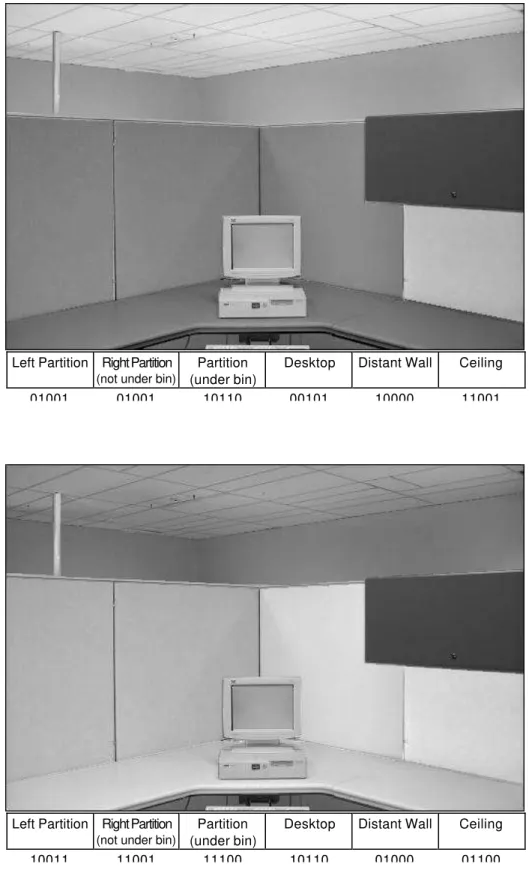
This experiment followed the general model from Johnston’s work, in which an analogy between Darwinian natural selection and the selection of the most attractive image is the basis of the technique. To begin the analogy of genetic survival of the fit, we need to define a “gene” for the image of a lit office space. In this case we have six luminous surfaces, as shown in Figure 1. We modify the luminance of each surface by changing the greyscale value in the digital image. There were 32 possible levels of luminance for each surface, arranged on an almost linear scale of increments. Each increment was equivalent to a change in 5 greylevels on the 256 level (8-bit) monochrome scale. Expressed in binary terms, the luminance of each surface varied between 00000 and 11111 (between 0 and 31 in decimal terms, which corresponded to a greyscale range of around 70 to 230, and a luminance range of

approximately 3 cd/m2 to 110 cd/m2, as presented to the participant). These binary expressions form a “luminance gene sequence” for the surface. So, for example, a luminance level of 9 for a surface, would be represented by the gene 01001, a level of 22 as 10110, and so on. The same can be done for each of the six surfaces, resulting in a 30-digit binary string, or in genetic language, a “phenotype”, which uniquely represents the combination of luminance in a particular image. Figure 3 illustrates two examples.

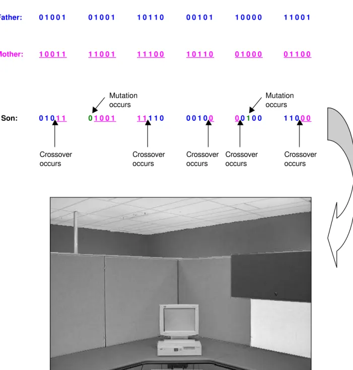
In the animal kingdom, according the Darwinian evolution, it is the fit individuals that survive, have most offspring, and thus most influence the next generation [PBS]. Applying a genetic algorithm in our experiment means that the most attractive (our measure of fitness) images are the ones that influence the next generation of images. Two of the most attractive images from a “population of images” are selected as “parent” images, and “reproduce” to create “child” images. Just as in the animal kingdom, these children are the product of their parents’ genes and display similarity to their parents’ features. We mimic sexual reproduction with operations on the binary strings called crossover and mutation (see Figure 4). In our version, each set of two parents produces two offspring; to follow the analogy, we call the two parents the “father” and the “mother”, and the two children the “son” and the “daughter”. To create the son’s phenotype, we start with the first binary digit in the father’s phenotype. For each digit, reading from left to right, we randomly test to see if crossover occurs, if it does not, the son’s digit is a copy of his father’s and the next digit of the father’s phenotype is tested for crossover. However, if crossover does occur the son’s digit is a copy of his mother’s and the next digit of the mother’s phenotype is tested for crossover. In our experiment, the possibility of crossover at each digit was set at 25%.

As in nature, there is always the (small) possibility of random mutation, which can be very helpful in bringing in new gene combinations which otherwise would not occur. For example, if both the father and the mother have a “0” as the 23rd digit (as in Figure 4), their offspring could never have a “0” without random mutation. Random mutations usually produce less fit individuals, and less attractive luminous scenes, but can occasionally get a gene line out of an “evolutionary dead-end”. Each of the son’s digits is tested for a random mutation; in our experiment, the possibility of random mutation at each digit was set at 4%. The creation of the daughter’s phenotype was created in exactly the same way as the son’s, except the process begins with the mother’s phenotype.

These two children are then presented to the participant and rated for attractiveness. If they are rated more highly than the lowest rated members of the existing population of images then they replace these lower rated members. The process of parent selection and creation of children continues, and the population, on average, becomes more attractive and more homogeneous. Genetic algorithms have

proven to be a much more efficient way of finding optimal solutions when the number of possible solutions is large, than simply searching the set of solutions by trial and error.

2.2.2 The software used in the experiment

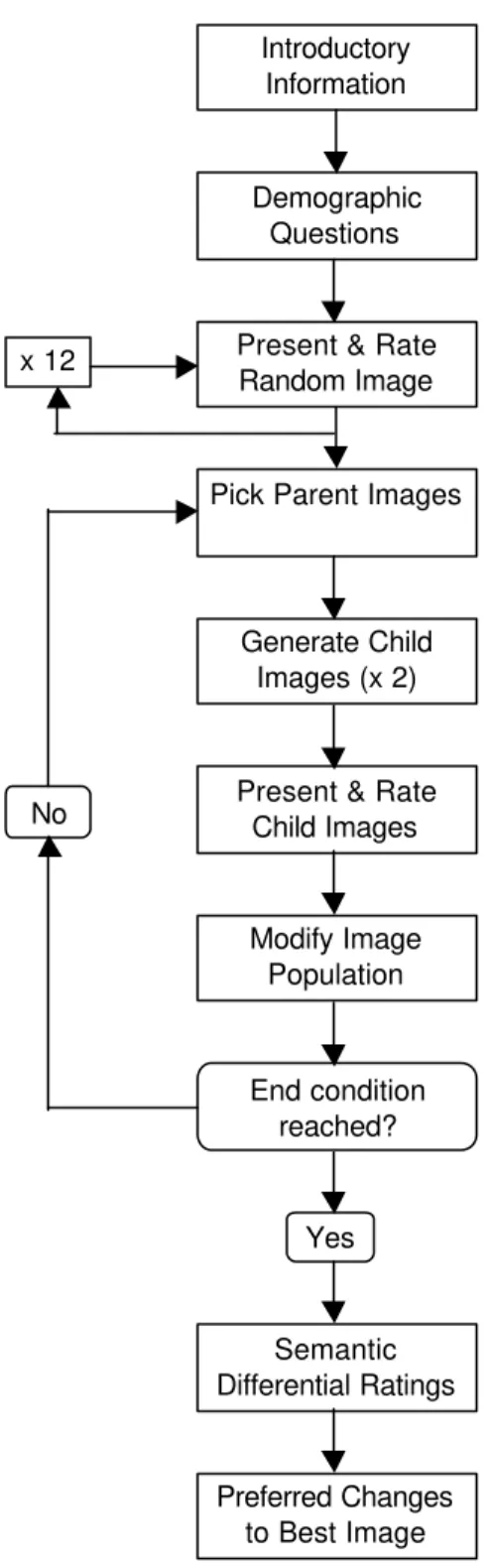
Software was written in Visual Basic to present the images, conduct the manipulation of surface luminances according to the genetic algorithm, to administer questionnaires, and to store data. A flow diagram for the software is shown in Figure 2.

After reading some introductory information, participants were first presented with a basic set of

demographic questions on: Sex, Age, Vision Correction, and Occupation. Following this, the main task of the session began, the rating of office images. The participants saw an initial set of 12 images, and were asked to rate each one for attractiveness, on a scale of 1 (least attractive possible) to 10 (most attractive possible). As in the entire session, images were presented one at a time, separated by at 15 seconds during which no image was present on the screen. Each of this initial set of images was simply a random combination of surface luminances. This set of 12 formed the initial population of images.

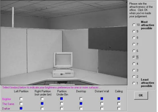
Then the genetic algorithm process began. Parent images were selected from the population. One parent was always the image with the highest rating. The second parent was selected randomly from the population, but the chance of being selected was weighted according to the image’s attractiveness rating. The child images were then presented and rated. After rating each child, an extra element was introduced to help the participant guide the genetic process – they were able to indicate for each surface whether they would prefer it brighter, the same, or darker (see interface in Figure 5). The next child was then created according to the genetic process described above, but it was also tested against the participant’s preference for each surface. If the child did not meet the set of preferences it was rejected and another child created and tested. The process continued until a satisfactory child was created. Nevertheless, it was not always possible, particularly as the images converged on the participant’s optimal image, to meet the participant’s preferences for all surfaces. In such cases the criteria for the number of surfaces that met the preferences was decreased from six to five to four and so on until a suitable child was created. The approach of guiding the genetic process was adopted by Johnston and shown to greatly increase the efficiency of the genetic algorithm [Caldwell & Johnston, 1991].

The process of parent selection and child creation continued until an end condition was reached. There were three conditions that ended the process:

• An image was given a rating of 10 (this could happen for one of the initial 12 images) • A participant expressed a preference for the same brightness for all six surfaces

• Neither of the two children created from a set of parents were rated more highly than the least attractive member of the prevailing population

Following the end condition, the participants were asked to rate the appearance of two images on a series of semantic differential (adjective pair) scales. The two images that were rated were the image with the highest rating in the final population (Best image), and the image rated third highest from the initial population (Comparison image). We wanted to test whether the genetic algorithm had in fact led to a preferred image that was significantly different from a non-optimal image. It seemed sensible that the comparison image be one of the initial random population so that its creation had not been influenced by the guided genetic algorithm. Nevertheless, we did not want to bias the comparison by choosing a comparison image that had an excessively low rating. For the appearance ratings, we chose 14 bipolar adjective pairs (bright - dim, uniform - non-uniform, interesting - monotonous, pleasant

- unpleasant, comfortable - uncomfortable, stimulating - subdued, radiant - gloomy, tense - relaxing, dramatic diffuse, spacious cramped, glaring notglaring, friendly hostile, simple complex, formal -casual). These adjective pairs were derived from previous research (Hendrick et al. 1977, Eissa &

presented in random order with each adjective pair presented one at a time next to the image. The participants gave their rating by moving a cursor between the two adjectives.

Finally, the Best image was recalled to the screen and the participant was asked to indicate, for each surface in turn, whether they would prefer it to be A lot Brighter, a little Brighter, No Change, a little

Darker, A lot Darker. The image did not change in response to this input. These ratings were another

way of assessing how optimal the Best image was.

2.3 The Experimental Space

The experiment was conducted using images projected onto a viewing screen using a Sharp model PG-C30XU LCD projector (see Figure 6 for diagram and photograph). Participants sat in a chair and viewed the image through a rectangular slot that could be adjusted in height. The inside of the space into which they looked was completely black except for the image, so there was no distracting surround. The participant had access to a keyboard and a mouse for answering questionnaires and making ratings.

The distance from the projector to the viewing screen affected both the size of the image and the maximum brightness of the surfaces. We wanted to make both as realistic as possible, but we were limited by the capabilities of the LCD projector. Our final choice gave an image that was 1.52m (60”) wide and 1.02m (41”) high, such that the computer monitor in the image was 0.20m (8”) corner to corner, or about 54% of full size. This allowed us to created surface luminances up to around 110 cd/m2, allowing for a wide range of realistic preferences. The luminance of the computer monitor in the image, which was constant for all images presented, was set to 53 cd/m2, typical of the luminance we measured for light grey on a real monitor; ANSI/IESNA RP-1 [1993] suggests typical screen luminances of 50 cd/m2.

2.4 Physical Measurements

Prior to beginning data collection we used a Topcon BM3 luminance meter to provide a calibration between grey level and luminance on the viewing screen. This calibration is show in Figure 7.

2.5 Participants

The 22 participants (10 male, 12 female) were lighting experts from all over North America (IESNA QVE committee) who were participating as part of workshop organised in conjunction with a nearby

conference. Participation was voluntary, and there was no reward for participation. Participant characteristics, from their self-reported demographic data, are shown in Table 1.

2.6 Experimental Procedure

At the start of the workshop potential participants were given a general description of the experiment both verbally and on paper, and asked to sign a consent form. We had two projection booths and so we were able to run two experimental sessions simultaneously. Therefore, two participants at a time were taken from the pool of 22 in an order that was determined by a random ballot conducted after the consent forms were signed. When not participating in the experiment, participants were either participating in a second experiment (to be reported elsewhere), or they took part in other lighting-related discussions as part of the workshop. The experimenter explained the procedure to the participants, and then invited them to take their places. All further information, instructions and tasks were presented on screen, though the experimenter remained close by to answer any arising questions. The entire procedure was submitted to and approved by our organisation’s Research Ethics Board. Completion of the on-screen part of the experimental procedure took a mean time of 20:47 (min:sec); s.d. = 5:14.

3. RESULTS

We present the results of the experiment as they pertain to specific questions we wanted to address.

3.1 Did the Genetic Algorithm Lead to a Highly Rated Image?

There were two direct measures pertaining to this question: the attractiveness ratings of the Best image (Figure 8), and the preferred changes in the Best image expressed at the end of the session (Figure 9). The mean attractiveness rating of the best image was 8.2 (s.d. = 1.4), and the modal rating was 9. When offered the opportunity to express a final preference for a change in surface brightnesses, almost 60% of the votes were for no change, and 95% for ‘No Change’ or ‘A little darker’ or ‘A little brighter’. A measure of the efficiency of the algorithm in reaching the best image is the number of images seen by the participants. No participant gave an attractiveness rating of 10 to any of the initial 12 random images, all progressed to the stage where images were generated according to the genetic algorithm. The mean number of images seen was 22.5 (s.d. = 5.3).

Although the Best image was not perfectly optimal (mean attractiveness rating was 8.2, not 10), it was rated very highly, and preferences for change were small. The Best image was achieved after viewing relatively few images. To summarize, the genetic algorithm was quite successful with the promise of future refinement.

3.2 Is the Most Attractive (Best) Image More Highly Rated than a Non-Optimal (Comparison) Image?

For the method to be useful, it must produce optimal images that are rated differently to non-optimal images, and in the expected manner – that is to say, observers must be able to reliably discriminate between preferred and non-preferred images. One way we explored this was through the semantic differential appearance ratings of the Best and Comparison images. Remember, both of these images differed from participant to participant (see Section 2.2.2). Figure 9 presents an example Best and Comparison image for one of the participants.

Figure 10 shows the mean ratings for the Best and Comparison images for each of the adjective pairs. We conducted statistical analyses to check for differences between the ratings. We first conducted an overall multivariate analysis of variance (MANOVA) to check for an overall difference across all adjective pairs. Statistical tests were within-subjects on a single independent variable: image type; with two levels: Best vs. Comparison. The overall difference was not significant (Wilks’ Λ = 0.194; R2ave = 0.36; F(14,8) = 2.37; p = 0.11). The lack of significance is not surprising, given the large number of

dependent variables (14 adjective pairs) and the relatively small number of participants (22). In fact, this ratio of participants to dependent variables is below that normally recommended, and it is therefore interesting to note the high value of the average variance explained (R2ave). It is not our usual practice to explore univariate effects – or differences on individual adjective pair ratings – if the overall MANOVA is not significant, as this runs the risk of Type I statistical errors. Nevertheless, because this is a pilot study of a new technique for lighting research, in this case we do report the results of the univariate tests. We believe that in this case the potential insight into the value of this new technique justifies the choice. The results of the statistical tests are shown in Table 2. The Best image is significantly brighter, more uniform, more pleasant, more comfortable, more subduing, more relaxed, less dramatic, more spacious, less glaring, more friendly and less complex.

These differences are as expected and, indeed, desirable. It is an important test of the method that participants can discriminate between stimuli in the expected manner. This result increases our

confidence that participants view the projected images in a similar way to the way they view real settings.

3.3 Are Images Perceived in the Same Way as Real Spaces?

Again, for this method to have value, it is important that participants interpret the patterns of light and dark in the viewed images as lighting of a real scene. We explored this with a factor analysis of the semantic differential appearance ratings. Factor analysis techniques find correlations between many scales, based on the supposition that responses to the individual scales represent facets of a response to a smaller number of higher level concepts. We expected that if the participants interpreted the images as the lighting of a real scene then the factor structure would be the same as the factor structure derived from ratings of a real scene. The image we used for this experiment was taken in a mock-up office space that had been previously used for a human factors study of lighting quality [Veitch & Newsham, 1998]. In that study nearly 300 participants experienced nine different office lighting designs (between-subjects) for a day, doing simulated office tasks and completing a variety of

questionnaires. The participants completed a similar set of semantic differential appearance artings on which factor analysis was performed.

The appearance ratings from our experiment were subjected to a factor analysis (principal components). The ratings of the best image and the comparison image were analysed independently, and the results are shown in Table 3. Also shown in Table 3 is the factor analysis of Veitch & Newsham [1998]. The ratings in Veitch & Newsham included more adjective pairs than we used in this study, only shared items are shown in the table, except for one adjective pair, ‘friendly-hostile’, which was used in the present study and not used in Veitch & Newsham. To facilitate comparison with the data from Veitch & Newsham, we forced a three factor solution on the data from this experiment. As in Veitch & Newsham we use a conservative criterion for factor loadings, highlighting only those unrotated loadings greater than 0.5.

The results show that the factor structure from the Best image is very similar to the factor structure from Veitch & Newsham, and we can be confident in using the same words to describe the concepts

associated with each factor. The differences in structure are small: for the Best image glaring-not glaring loads on Factor 1, whereas it did not load (>0.5) on any factor in Veitch & Newsham; dramatic-diffuse loads on Factor 2, whereas it did not load (>0.5) on any factor in Veitch & Newsham. For the Best image, interesting-monotonous and subdued-stimulating load on Factor 2 as well as Factor 1, whereas they loaded on Factor 1 only in Veitch & Newsham.

The factor structure from the Comparison image is much more complex and compares poorly with the data from Veitch & Newsham. There are many more adjective pairs that load on different factors, and load on more than one factor, and simple labels for the concepts associated with these factors are difficult to derive.

One explanation for these results is that participants did perceive the Best image as a realistic lit scene and produced a factor structure similar to that derived from evaluations of a real scene. On the other hand, the Comparison image was not perceived as realistic. Figure 9 demonstrates why this might be so. The pattern of light and dark surfaces in the Best image corresponds well with what might occur in a real office space where reflectances are reasonably uniform and the lighting system is simple. It is clear that the pattern of light and dark surfaces in the Comparison image would be very difficult to achieve in reality except by using very non-uniform reflectances or a set of very focussed luminaires, both of which would be highly unusual in this setting.

The fact that the participants’ Best image seems to have been perceived as realistic supports the validity of the method for deriving preferred luminous patterns for real spaces.

3.4 Are Preferred Luminances and Ratios the same as Those Derived from Experiments in Real Spaces?

Table 4 presents a summary of the luminance information from the 22 Best images. Data is presented for the six surfaces that were independently manipulated, for meaningful combinations of surfaces, and for important ratios.

To check further the validity of this method we compared the preferred luminous conditions in the Best images to those derived from human factors experiments in real spaces. All of the studies we refer to in this section excluded daylight and derived preferences for electric lighting only, analogous with our study. Veitch & Newsham [2000] conducted a study in the same laboratory space in which the photograph used in this study was taken. Participants had dimmable control over three lighting circuits (one indirect and two direct) as well as on-off control over an undershelf task light. Participants

occupied the space for an 8-hour day during which they conducted typical office tasks, predominantly computer based. Half the sample of 94 had control at the start of the day, the other half at the end of the day. One value reported was the mean luminance in an area that included the partitions behind the computer and under a binder bin, part of the desktop and part of the binder bin – this area was chosen to represent the 40o horizontal band of field of view from Loe et al. [1994]. The median luminance chosen by participants in this area was 39.2 cd/m2 (min. = 11.5, max. = 61.0, s.d. = 12.0) [Veitch & Newsham, 2000]. The nearest equivalent value from this study is probably the mean of ABCD (all the partitions and desktop taken together, median = 46.8 cd/m2 (min. = 32.8, max. = 73.7, s.d. = 9.3). Note that the value from Veitch & Newsham included part of the binder bin – a very dark area (< 10 cd/m2) occupying around 1/12 of the field of view, which was not included in the mean of ABCD.

Removing the binder bin from the Veitch and Newsham area would increase the median luminance to by around 10%, making the comparison even better.

We can also make an approximate comparison of preferred desktop luminance. Veitch and Newsham [2000] reported illuminance at a single location. If we assume this was representative of the average for the whole desktop, and we assume it was a diffuse (it was actually described as low gloss, ρ=0.503), then we can derive desktop luminance. The luminance thus derived, median = 66.1 cd/m2 (min. = 13.3, max. = 116.1, s.d. = 24.3), compares well with the preferred desktop luminance from this study, median = 55.1 cd/m2 (min. = 10.3, max. = 103.5, s.d. = 28.1).

Berrutto et al. [1997] also gave participants dimming control over a variety of luminaires in small private offices. Exposures were limited to 20 minutes, and data were collected separately for different tasks. They concluded that for non-VDT tasks wall luminance at eye level should be around 60-65 cd/m2, and for VDT tasks the luminances around the screen should be equal or lower than the luminance of the screen. In our study, the screen luminance was 53 cd/m2 and the immediate surround luminance, perhaps best expressed by the average of AB, had a median of 45.4 cd/m2. They described their furniture to include “one slightly glossy grey desk (50% reflectance).” If we make the same diffuse reflection assumptions as above, then, for non-VDT tasks, mean desktop luminance = 65.4 cd/m2 (min. = 15.3, max. = 176.9), and, for VDT tasks, mean desktop luminance = 43.8 cd/m2 (min. = 9.7, max. = 87.1). These values bracket the results from our study.

Van Ooyen et al. [1987] presented participants with different office luminous environments by

manipulating light distributions and changing the reflectivity of surfaces; working plane illuminance was maintained at around 750 lux. The spaces were private two-person offices, and data were collected separately for different tasks. For non-VDT tasks, preferred wall luminances were 30 to 60 cd/m2, and preferred working plane luminances were 45 to 105 cd/m2. For VDT work the values were reduced: preferred wall luminances were 20 to 45 cd/m2, and preferred working plane luminances were 40 to 65 cd/m2. These preferred luminances correspond well with our median luminances from the Best images. Van Ooyen et al. reported that the preferred ratio of working plane luminance to wall luminance was 1.33:1, our equivalent ratio D:ABC was 1.21:1, which is remarkably similar.

Loe et al. [1994] had observers rate a small conference room from a point of view equivalent to the room’s entrance. Lighting conditions were manipulated by the experimenters using a variety of luminaires. They concluded that for ‘visual lightness’ the preferred average luminance in a horizontal band of field of view 40o wide should be >= 30 cd/m2. It is difficult to make a direct comparison to our data as the image participants evaluated in our study did not fill the entire field of view and was entirely encompassed by Loe et al.’s 40o band. The median value of all six surfaces in the Best images in our experiment was >30 cd/m2, and the mean of all six surfaces was > 30 cd/m2 for all 22 participants’ Best images (min. = 39.7 cd/2).

Taken together, these comparisons show that the preferred luminances derived from our study compare well with the preferred luminances from other studies using more traditional methods.

3.5 What are the Recommended Luminances Derivable from this Study?

Our study shows that that there is a wide variety in the preferences of individuals. This is a common finding in lighting research, which suggests that the best way to maximise satisfaction with lighting is to offer individual control [Newsham & Veitch, 2001]. Several studies have demonstrated that individual control over lighting can also improve overall environmental satisfaction, lower lighting energy

consumption, and allow the occupant to tailor lighting to tasks [Boyce et al, 2000; Jennings et al., 2000, Maniccia et al., 1999; Carter et al., 1999].

Nevertheless, individual control is not always available. When lighting is fixed and the same for all, the recommended luminances for the space are simply the averages for each of the surfaces. These values are shown numerically in Table 4, and pictorially in Figure 111. It is interesting to compare this with the base image in Figure 1 in which each surface is in the middle of the range of possible values. In the average preferred image the partitions behind the computer are slightly darker, whereas the partition below the storage bin is slightly lighter – in reality this could only be achieved with an undershelf task light. The desktop is slightly lighter than the partitions, as is the distant wall. The brightest surface of all is the ceiling.

4. FURTHER DISCUSSION

Following data collection, which took place on a single day, many of the participants met together with the experimenters to discuss the experiment. Several of the participants thought that the setting and stimulus were very artificial and doubted that the results would have meaning or be applicable in real settings. It is therefore particularly pleasing that the results we did obtain are very promising, and similar to those obtained from experiments in real settings – our participants were clearly not biased towards obtaining a positive result!

Some participants were frustrated that they could only express their preferences by guiding the

evolution process – which did not always give them exactly the result they were expecting – rather than by directly manipulating the brightness of each surface. However, one of the advantages of the genetic algorithm is that it is not deterministic and includes some randomness. This forces participants to consider luminous environments they are not familiar with but which might have advantages, rather than allowing them to immediately select a pattern of brightnesses according to a pre-existing bias. Also, this study involved the manipulation of only six surfaces, direct manipulation might not be practical in future studies involving many more variables.

In this study we changed the luminance of objects uniformly across their surface, which emphasized the independence of these changes from any luminaires. In addition, the surface luminances were

independent of each other, there were no direct inter-reflections. Furthermore, no luminaires were visible

1

The translation to the image is only approximate because the numerical average does not necessarily correspond with an integer gene value.

in the viewed image. This was deliberate; we are interested in participants’ fundamental preferences of light and dark without concern as to how this might be achieved in reality. Nevertheless, there is a danger in this: in reality, surface luminances can be changed via illumination or by changing reflectance, and the two are not necessarily perceptually equivalent (see references in Moeck [2001]). Therefore, our approach risks confusing the participant when viewing the scene: are they observing lighting manipulations, reflectance manipulations, or a combination of both? This could be a mechanism for reducing the reality of the experience. Nevertheless, we reiterate that our results compare well with those obtained in real settings. It is also worth noting that natural-looking inter-reflections could be achieved in our study indirectly. A brighter partition would not directly produce a brighter desktop, but a brighter desktop could be achieved in future generations of the image. All the same, in future work we intend to include realistic luminaires and inter-reflections.

In Section 3.3 we noted that the factor structure from the semantic differential appearance ratings for the Best image was similar to the structure from ratings in a real setting, where as the factor structure from the Comparison image was not. We concluded that the Best image was perceived as realistic whereas the Comparison image was not. To investigate this further in future work, we plan to add a third image to the appearance rating part of the experimental procedure. This third image will be selected to be realistic: possibilities include the inverse of a participant’s Best image, the average Best image from this study, or a suitably modified image from a real setting. If the factor structure of the this third image is similar to that from the Best image and to ratings from a real setting we can have more confidence that participants perceive their preferred, Best image as realistic.

5. CONCLUSIONS

The main findings of this experiment are:

• The genetic algorithm method is successful in obtaining participant’s preferred luminance patterns (Best image) in a greyscale image of an office space.

• Participants were sensitive to manipulation of luminances in the image, such that appearance ratings of a participant’s Best image and a non-optimal Comparison image were significantly different in the expected directions.

• The factor structure of the appearance ratings for the Best image is similar to the factor structure for ratings given by occupants of an equivalent real space.

• The preferred surface luminances from the projected images are similar to those from experiments in real settings.

All of these findings indicate that the genetic algorithm method of deriving preferred patterns of luminance, realised by projecting close to full-scale images at realistic luminances, has promise. Future work should further explore this method using larger number of participants drawn from a more representative population (i.e., not lighting experts). If future work reinforces our findings that the results of this method are equivalent in many ways to the results from real settings, this method might be able to replace much more expensive experiments in real settings in some instances.

6. ACKNOWLEDGEMENTS

This work was sponsored by the National Research Council Canada (NRC), the Project on Energy Research & Development, and Public Works & Government Services Canada (PWGSC). The authors are grateful for the technical help provided by Marcel Brouzes (NRC) and programming help from Philippe Marchand. Dr. Victor Johnston for guidance on the use of genetic algorithms for human factors research. We also thank Dr. Morad Atif (NRC), Ivan Pasini (PWGSC) and Karen Pero (PWGSC) for their support. This experiment was conducted as part of a QVE/MOQ research workshop, and we acknowledge the support of the IESNA QVE/IALD MOQ committee, particularly the hard work of Peter Ngai and Linda Owens of Peerless Lighting.

7. REFERENCES

ANSI/IESNA. 1993. RP-1, Office Lighting, American National Standard, Illuminating Engineering Society of North America (New York, USA).

Ashdown, I. 1994. “Non-imaging optics design using genetic algorithms”, Journal of the Illuminating

Engineering Society, Winter, pp. 12-21.

Berrutto, V.; Fontoynont, M.; Avouac-Bastie, P. 1997. “Importance of wall luminance on users satisfaction: pilot study on 73 office workers”. Proceedings of Lux Europa – 8th European Lighting Conference (Amsterdam), pp. 82-101. Arnhem: NSVV.

Boyce, P.R.; Eklund, N.H.; Simpson, S.N. 2000. “Individual Lighting Control: Task Performance, Mood, and Illuminance”, Journal of the Illuminating Engineering Society, Winter, pp. 131-142.

Caldwell, C.; Johnston, V.S. 1991. “Tracking a criminal suspect through ‘Face-Space’ with a genetic algorithm”, Proceedings of the 4th International Conference on Genetic Algorithms (San Diego), pp. 416-421. San Mateo: Morgan Kaufmann

Carter, D.J.; Slater, A.I.; Moore, T. 1999. “A Study of occupier controlled lighting systems”, Proceedings of the 24th Session of CIE (Warsaw), pp. 108-110. Vienna, Austria: Commission Internationale de l’Eclairage.

Chutarat, A.; Norford, L.K. 2001. “A new design process using an inverse method: a genetic algorithm for daylighting design”, Proceedings of IESNA Annual Conference (Ottawa), pp. 217-229. New York: Illuminating Engineering Society of North America.

Danford, S.; Willems, E.P. 1975. “Subjective responses to architectural displays,” Environment and

Behavior 7(4), pp. 486-516.

Daniel, T.C.; Meitner, M.M. 2000. “Representational validity of landscape visualizations: the effects of graphic realism on perceived scenic beauty of forest vistas,” Journal of Environmental Psychology 21,

pp. 61-72.

Eissa, H.; Mahdavi, A. 2001. “Subjective evaluation of architectural lighting via computationally rendered images,” Proceedings of IESNA Annual Conference (Ottawa), pp. 547-558. New York: Illuminating Engineering Society of North America.

Eklund, N.H.; Embrechts, M.J. 2001. “Multi-objective optimization of spectra using genetic algorithms”,

Journal of the Illuminating Engineering Society, Summer, pp. 65-72.

Hendrick, C.; Martyniuk, O.; Spencer, T.J.; Flynn, J.E. 1977. “Procedures for investigating the effect of light on impression: simulation of a real space by slides,” Environment and Behavior 9 (4), pp. 491-510.

Jennings, J.D.; Rubinstein, F.M.; DiBartolomeo, D.; Blanc, S.L. 2000. “Comparison of control options in private offices ...”, Journal of the Illuminating Engineering Society, Summer, pp 39-60. (also available at http://eetd.lbl.gov/btp/450gg/)

Johnston, V.S. 1999. Why We Feel, Perseus Books (Reading, MA, USA).

Johnston, V.S.; Franklin, M. 1993. “Is beauty in the eye of the beholder?,” Ethology and Sociobiology

14, pp. 183-199.

Kawai, J.K.; Painter, J.S.; Cohen, M.F. 1993. “Radioptimization - goal based rendering”, Proceedings of SIGGRAPH (Anaheim), pp.147-154.

Loe, D. L.; Mansfield, K. P.; Rowlands, E. 1994. “Appearance of lit environment and its relevance in lighting design: experimental study,” Lighting Research and Technology 26(3), pp. 119 – 133.

Maniccia, D.; Rutledge, B.; Rea, M.S.; Morrow, W. 1999. “Occupant Use of Manual Lighting Controls in Private Offices”, Journal of the Illuminating Engineering Society, Summer, pp. 42-56.

Moeck, M. 2001. “Designed appearance lighting - revisited”, Journal of the Illuminating Engineering

Society, Summer, pp. 53-64.

Newsham, G.R.; Veitch, J.A. 2001. "Lighting quality recommendations for VDT offices: a new method of derivation," Lighting Research and Technology, 33 (2), 2001, pp. 97-116.

PBS. A resource for a description of Darwin’s work, and other material to put it in context can be found at http://www.pbs.org/wgbh/evolution/library/02/index.html

Schoeneman, C.; Dorsey, J.; Smits, B.; Arvo, J.; Greenberg, D. 1993. “Painting with light”, Proceedings of SIGGRAPH (Anaheim), pp.143-146.

Van Ooyen, M.H.F.; van de Weijgert, J.A.C; Begemann, S.H.A. 1987. “Preferred luminances in offices”. Journal of the Illuminating Engineering Society, Summer, pp. 152 - 156.

Veitch, J.A.; Newsham, G.R. 1998. “Lighting quality and energy-efficiency effects on task

performance, mood, health, satisfaction and comfort”. Journal of the Illuminating Engineering Society, Winter, pp. 107 - 129.

Veitch, J.A.; Newsham, G.R. 2000. “Preferred luminous conditions in open-plan offices: research and practice recommendations”, Lighting Research and Technology, 32 (4), pp.199-212.

Table 1. Participant characteristics. Total

responses

Sex Female Male

22 12 10 Age 18-29 30-39 40-49 50-59 60-69 70+ 22 1 8 7 5 1 0 Correction Lenses None Reading Glasses Distance Glasses Bi- or Trifocal Lenses Gradual or Multifocal Lenses Contact Lenses 22 5 4 5 2 2 4 Principal Occupation

Research Education Design Manufacturin g

Marketing/ Sales

Other

22 4 4 6 5 2 1

Table 2. Result of MANOVA and univariate effects on appearance ratings. Statistical tests were within-subjects on a single independent variable: image type; with two levels: Best vs. Comparison

Effect r2 F(1,21) p bright - dim 0.29 8.62 <0.01 uniform - non-uniform 0.55 26.08 <0.01 interesting - monotonous n.s. pleasant - unpleasant 0.55 25.17 <0.01 comfortable - uncomfortable 0.55 26.04 <0.01 stimulating - subdued 0.18 4.70 <0.05 radiant - gloomy n.s tense - relaxing 0.48 19.74 <0.01 dramatic - diffuse 0.52 22.73 <0.01 spacious - cramped 0.35 11.06 <0.01 glaring - not-glaring 0.35 11.29 <0.01 friendly - hostile 0.34 10.59 <0.01 simple - complex 0.54 24.24 <0.01 formal - casual n.s.

Table 3. Results of factor analysis on semantic differential appearance ratings for Best image and Comparison image. Also shown is a similar analysis from Veitch & Newsham [1998], labelled ‘V&N’ in the table. A * in the table indicates an unrotated factor loading of >0.5.

Factors & Unrotated Component Loadings

Factor 1 Factor 2 Factor 3

V&N best comp. V&N best comp. V&N best comp. Concept associated with factor

→ Visual Attractio n Visual Attractio n Complexit y Complexit y Brightnes s Brightnes s ADJECTIVE PAIR ↓

friendly-hostile N/A * * N/A N/A

pleasant - unpleasant * * * interesting - monotonous * * * * comfortable - uncomfortable * * * subdued - stimulating * * * * gloomy - radiant * * * * spacious - cramped * * * tense - relaxing * * * * nonuniform – uniform * * * complex - simple * * * bright - dim * * * *

glaring - not glaring * *

dramatic - diffuse * * *

formal - casual

% Total Variance explained

Veitch & Newsham [1998] 44.2 Best image 73.7 Comparison Image 69.3

Table 4. Luminances derived from the 22 Best images. Values for the six directly manipulated surfaces are shown, as well as combinations of surfaces, and important ratios.

Median (s.d.) Min. Max.

Left Partition (A) cd/m2 41.1 (17.2) 16.4 82.9

Right Partition (not under bin) (B) cd/m2 49.0 (18.6) 13.6 89.7

Partition (under bin) (C) cd/m2 _{53.3 (24.2) 2.6 94.1}

Desktop (D) cd/m2 55.1 (28.1) 10.3 103.5

Distant Wall (E) cd/m2 _{52.6 (24.2) 10.4 101.7}

Ceiling (F) cd/m2 62.7 (22.9) 14.0 95.9 mean of ABCD cd/m2 46.8 (9.3) 32.8 73.7 mean of ABC cd/m2 _{46.2 (12.6) 30.0 76.5} mean of AB cd/m2 45.4 (16.3) 17.4 86.3 A:B 0.88 (0.58) 0.52 3.25 B:C 1.06 (4.00) 0.18 19.46 D:ABC 1.21 (0.84) 0.18 3.17 AB:E 0.91 (0.91) 0.18 4.52 E:F 0.88 (0.85) 0.16 4.13 VDT screen:ABC 1.17 (0.29) 0.71 1.80 VDT screen:D 0.98 (1.09) 0.52 5.26 AB:F 0.70 (0.89) 0.36 4.04 D:ABCD 1.15 (0.52) 0.33 2.05

Figure 1. The base image used in the experiment, and the six surfaces that were independently manipulated in luminance.

Introductory Information Demographic Questions Semantic Differential Ratings

Present & Rate Random Image x 12

Pick Parent Images

Generate Child Images (x 2)

Present & Rate Child Images End condition reached? Yes No Modify Image Population

Figure 2. Overall flow diagram of software used in experiment

Preferred Changes to Best Image

Left Partition Right Partition

(not under bin)

Partition (under bin)

Desktop Distant Wall Ceiling

01001 01001 10110 00101 10000 11001

Left Partition Right Partition

(not under bin)

Partition (under bin)

Desktop Distant Wall Ceiling

10011 11001 11100 10110 01000 01100

Figure 3. Two example combinations of surface luminances. Below each is the binary phenotype that represents the combinations of luminances, made up of 5-digit genes for each surface.

Father: 0 1 0 0 1 0 1 0 0 1 1 0 1 1 0 0 0 1 0 1 1 0 0 0 0 1 1 0 0 1

Mother: 1 0 0 1 1 1 1 0 0 1 1 1 1 0 0 1 0 1 1 0 0 1 0 0 0 0 1 1 0 0

Son: 0 1 01 1 01 0 0 1 1 11 1 0 0 0 1 00 0010 0 1 1 00 0

Figure 4. Crossover and mutation from parents’ phenotypes (see Figure 3) to create a son phenotype; mother’s genes are underlined. Resulting combination of surface luminances is shown.

Crossover occurs Crossover occurs Crossover occurs Crossover occurs Crossover occurs Mutation occurs Mutation occurs

Figure 5. Interface for the experimental task. Participants rated the image for overall attractiveness. They then used the boxes at the bottom to indicate their brightness preference for each surface.

Figure 6. Experimental set-up. Participants viewed the projected image through a port-hole (photo on left). The space into which they looked was black except for the projected image (photo on right, with

front wall removed). Diagram shows side elevation, approximately to scale.

2.72m (107”) 3.66m (144”) 1.63m (64”) 3.20m (126”) LCD projector Computer Projection screen viewport

Figure 7. Calibration of projector screen luminance vs. image pixel grey level.

Figure 8. Histogram of the attractiveness rating of the Best image (n=22).

y = 0.0012x2 + 0.244x - 20.5 R2 = 0.9959 0 20 40 60 80 100 120 0 50 100 150 200 250 300

grey level

luminance (cd/m2)

Attractiveness Vote for Best Image

Figure 8. Histogram of the preference for change in brightness of the six surfaces in the image, for the Best image. Data for all surfaces are grouped (n=132).

Figure 9. Example of a Best image (in this case, given an attractiveness rating of 8) and its Comparison image (which received an attractiveness rating of 6).

0 20 40 60 80

A lot _{darker A little darker} No

Change A little brighter A lot brighter No Vote

Surface Change Vote

Figure 10. Comparison of mean semantic differential appearance ratings for the Best image and its Comparison image (n=22). A star next to the point representing the mean rating of the Best image

indicates a significant difference for that adjective pair.

Figure 11. (Approx.) Average preferred luminance.

bri -dim uni -non int -mon ple -unp com-unc sti -sub rad -glo ten-rel dra -dif spa-cra gla -not fri -hos sim -com for-cas

Mean Rating

glaring _friendly simple formal non-uniform monotonous unpleasant uncomfortable subduing gloomy relaxed diffuse cramped not glaring hostile complex casual

* * * * * * * * * * *