Dynamic hysteresis modelling of entangled cross-linked fibres in shear

HAL Id: hal-01758580

https://hal.archives-ouvertes.fr/hal-01758580

Submitted on 4 Apr 2018

HAL is a multi-disciplinary open access

archive for the deposit and dissemination of

sci-entific research documents, whether they are

pub-lished or not. The documents may come from

teaching and research institutions in France or

abroad, or from public or private research centers.

L’archive ouverte pluridisciplinaire HAL, est

destinée au dépôt et à la diffusion de documents

scientifiques de niveau recherche, publiés ou non,

émanant des établissements d’enseignement et de

recherche français ou étrangers, des laboratoires

publics ou privés.

Dynamic hysteresis modelling of entangled cross-linked

fibres in shear

Elsa Piollet, Dominique Poquillon, Guilhem Michon

To cite this version:

Elsa Piollet, Dominique Poquillon, Guilhem Michon. Dynamic hysteresis modelling of entangled

cross-linked fibres in shear.

Journal of Sound and Vibration, Elsevier, 2016, 383, pp.248-264.

To cite this version :

Piollet, Elsa and Poquillon, Dominique

and Michon, Guilhem

Dynamic hysteresis modelling of entangled cross-linked fibres in shear.

(2016) Journal of Sound and Vibration, vol. 383. pp. 248-264.

ISSN 0022-460X

O

pen

A

rchive

T

OULOUSE

A

rchive

O

uverte (

OATAO

)

OATAO is an open access repository that collects the work of some Toulouse researchers

and makes it freely available over the web where possible.

This is an author’s version published in :

http://oatao.univ-toulouse.fr/19782

Official URL :

https://dx.doi.org/10.1016/j.jsv.2016.06.023

Any correspondence concerning this service should be sent to the repository administrator :

Dynamic hysteresis modelling of entangled cross-linked fibres

in shear

Elsa Piollet

a,n

, Dominique Poquillon

b

, Guilhem Michon

c

a_{CREPEC, École Polytechnique, Dep. Mechanical Engineering, P.O. Box 6079 Station Centre-Ville, Montréal (Québec), Canada H3C 3A7} b_{Université de Toulouse, CIRIMAT, INPT-ENSIACET, 4 allée Emile Monso, BP 44362, 31432 Toulouse, France}

c_{Université de Toulouse, ICA, ISAE, 10 avenue Edouard Belin, BP 54032, 31055 Toulouse, France}

a r t i c l e

i n f o

Keywords: Fibres Entangled Hysteresis Dry friction Dahl model

a b s t r a c t

The objective of this paper is to characterize and model the vibration behaviour of entangled carbon fibres cross-linked with epoxy resin. The material is tested in shear, in a double lap configuration. Experimental testing is carried out for frequencies varying from 1 Hz to 80 Hz and for shear strain amplitudes ranging from 5 ! 10" 4_{to 1 ! 10}" 2_{. Measured}

shear stress–strain hysteresis loops show a nonlinear behaviour with a low frequency dependency.

The hysteresis loops are decomposed in a linear part and three nonlinear parts: a dry friction hysteresis, a stiffening term and a stiction-like overshoot term. The Generalized Dahl Model is used in conjunction with other hysteresis models to develop an appropriate description of the measured hysteresis loops, based on the three nonlinear parts. In particular, a new one-state formulation of the Bliman–Sorine model is developed. A new identification procedure is also introduced for the Dahl model, based on the so-called backbone curve. The model is shown to capture well the complex shapes of the measured hysteresis loops at all amplitudes.

1. Introduction

Entangled materials are composed of flexible fibres with random or chosen orientations. Their properties are linked to the fibre orientation, the fibre density as well as the type of contacts between the fibres[1]. One of the interesting properties of fibrous materials is their ability to dissipate energy through friction between fibres, as shown by Poquillon[2]in static compression for example.

Recently, Mezeix[3,4]introduced a new material in which glass, aramid or carbon fibres are first entangled and then cross-linked with epoxy resin. Creating permanent links between some of the fibres increases the stiffeness of the material compared to entangled fibres. This makes the entangled cross-linked material a suitable core for sandwich structures. Sandwich structures are three-layered structures in which two facesheets are separated by a core, which needs to be both lightweight and stiff enough to reach good stiffness-to-weight ratios.

So far, studies on this entangled cross-linked material have focused mainly on its process and static properties in compression, tension and bending[3–6]. A first study on the vibration properties of sandwich structures with entangled core material has shown increased damping as compared to classical core materials such as honeycomb or foams [7].

n

Corresponding author.

However, the intrinsic behaviour of the material has not been investigated. Moreover, the vibration response was presented for one amplitude of excitation only, while fibrous materials are known to exhibit nonlinear behaviours[8]. A material study taking nonlinearity into account is thus necessary.

In order to describe a dissipative nonlinear behaviour, hysteresis models can be used. Recently, Al Majid and Dufour

[9,10]introduced the Generalized Dahl Model, which allows the representation of hysteresis loops with complex shapes, relying on the description of their asymptotes. However, the expressions of the asymptotes have to be assumed, which is not straightforward for complex shapes.

This paper presents the first study of the vibration behaviour of entangled cross-linked carbon fibres to the authors' knowledge. Moreover, an original combination of existing hysteresis models is introduced, and the proposed method can be applied to a large set of physical phenomena.

The paper is organized as follows.Section 2describes the entangled cross-linked material and the experimental set-up for shear testing. InSection 3, the measured shear stress–strain hysteresis loops are analysed and are interpreted in terms of the activated deformation mechanisms.Section 4details the development of an adapted hysteresis model to describe the measured hysteresis loops.Section 5presents identification procedures for the model. Finally, inSection 6the parameters of the model are obtained and discussed.

2. Material and set-up 2.1. Material fabrication

In the present study, the entangled cross-linked material is made with carbon fibres, as they provide higher perfor-mances compared to glass or aramid fibres, albeit for a higher cost. They are widely used in aerospace applications along with epoxy resin, in particular in carbon-epoxy sandwich facesheets. The carbon fibres have a diameter of 7

μ

m, a Young's

modulus of 240 GPa and a bulk density of 1770 kg/m3_.

Epoxy resin is used for cross-linking because of its wide use in aeronautical applications. An injection resin with a hardener is used.

The entangled cross-linked material is made following the process introduced by Mezeix[3,4]:

#

The fibres are first cut to a length of 31 mm. They are then separated and entangled in a 64 L blower room with an air flux at a 5 bar pressure applied manually. The density of the entangled material before cross-linking is 150 kg/m3_{, which} represents a fibre volume fraction of 8.5 percent.

#

_{The entangled fibres are then cross-linked by projecting epoxy resin with a paint spray gun at a 2 bar pressure. The resin}

droplets bond part of the contacts between the fibres. The density of epoxy resin in the final material is 30 kg/m3_{, a low} density as compared to the fibre density.

#

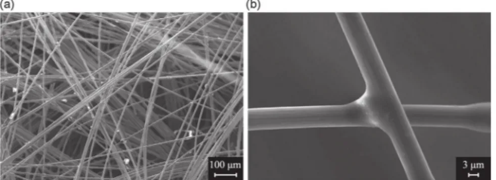
_{The samples are then polymerized in a mold at 70 °C during 8 h.}

Fig. 1shows a scanning electron microscope observation of the material after polymerization. As can be observed, the fibres are surrounded by air rather than a matrix: epoxy resin creates links at the contact between some fibres, while at other contacts fibres remain free to move with respect to one another.

2.2. Experimental set-up

As the entangled cross-linked material is intended to be used as a sandwich core material, its shear behaviour is of prime interest[11]. The shear set-up is presented inFig. 2. Two samples are tested together in a double lap configuration to ensure shearing only. The set-up includes a linear vertical motor above the samples, and a load cell under the samples. The

Fig. 1. Scanning electron microscope observation of entangled cross-linked carbon fibres: (a) general view showing cross-linked and free contacts and (b) zoom on a typical cross-linked contact between two carbon fibres.

dimensions of each sample are h $ l $ L ¼ 20 mm $ 40 mm $ 60 mm. The samples are glued to 3 mm thick aluminium plates on each side. Two of the plates are bolted together at the centre of the set up and linked to the vertical motor. The external plates are clamped to the load cell through two steel brackets on a thick aluminium support.

A controlled vertical displacement of amplitude u0and frequency f is applied to the two central plates by the electric motor:

uðtÞ ¼ u0sin ð2

π

ftÞ (1)

which leads to a shear strain

γ

in the samples, as described inFig. 3. Assuming that shear is constant through the thickness of the samples, the engineering shear strain in small deformations is:

γ

ð Þ ¼t uðtÞ

h ¼

γ

0sin 2ð

π

ftÞ (2)

where h is the thickness of each sample.

The resulting force F at the base of the set up is measured by a load cell under the samples. The shear stress is obtained by dividing the force applied on each sample, F=2, by the surface through which it is applied, S ¼ l $ L, resulting in the following expression:

τ

ð Þ ¼t FðtÞ

2S (3)

After fabrication and before making further measurements, the samples are excited at an amplitude of

γ

0¼ 1 ! 10" 2and

a frequency of 20 Hz. During the first cycles, the measured shear stress–strain response evolves with the number of cycles applied. The stiffness of the samples decreases, and damping increases. After around 40,000 cycles, the behaviour stabilizes. Further cycling at amplitudes under

γ

0¼ 1 ! 10" 2will not modify the shear behaviour any more. Moreover, this pre-cycled

behaviour is stable in time, and new series of testing after several days show the same properties for the pre-cycled samples. All measurements presented in this article are made after this pre-cycling.

Fig. 2. Double lap shear set-up: (a) schematic principle and (b) experimental set-up.

Fig. 3. Shear strain γ in each sample resulting from the applied displacement u. F is the load measured at the load cell under the samples: as the assembly is symmetrical and two identical samples tested together, it is assumed that the force applied to each sample is F=2.

3. Measurements and first analysis

Measurements are made for an amplitude range of

γ

0¼ 5 ! 10" 4 to

γ

0¼ 1 ! 10" 2 (u0¼ 5

μ

m to u0¼ 100

μ

m) and a

frequency range of 1 Hz to 80 Hz. These ranges are limited by the set-up. The amplitude range corresponds to small deformations (

γ

0⪡1) with a large range of variations, the minimum being 20 times smaller than the maximum. The

fre-quency range is low compared to the frefre-quency range of interest in structural vibrations (up to 1000 Hz or above). However it allows transitioning from the previous static studies[4,5]to vibrations studies. Testing at 1 Hz is close to static testing, while testing from 20 Hz to 80 Hz should permit highlighting vibration specific phenomena.

3.1. Linear part

Fig. 4shows a shear stress–strain hysteresis loop measured at an amplitude of

γ

0¼ 1 ! 10" 2and a frequency of 20 Hz for

a set of two samples. The loop is composed of a linear part, represented by the dashed line on the figure, and a hysteresis part that carries the dissipative and nonlinear behaviour of the material. Previous studies on the behaviour of entangled fibres with and without cross-links[6]have shown that cross-links increase significantly the stiffness of the material. Thus, the linear part of the measured hysteresis can be assumed to come mainly from the carbon fibre network created by the epoxy resin bondings achieved at a large number of cross-links.

Keeping in mind this linear part, the study and following figures will focus on the hysteresis part of the stress defined as follows:

τ

H¼

τ

" G1

γ

(4)

where G1is a constant parameter that will be identified inSection 6. 3.2. Hysteresis loops

Fig. 5shows

τ

H plotted against

γ

for amplitudes ranging from

γ

0¼ 5 ! 10" 4 to

γ

0¼ 1 ! 10" 2 for the same set of two

samples. As can be observed, the shapes of the hysteresis loops vary strongly with amplitude, which indicates material nonlinearity.

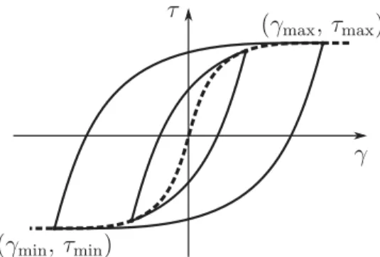
Fig. 6shows the loops along with a curve linking the extrema of the loops. This curve is called the backbone curve in the fields of material study and control: in some cases, it represents the response of the tested system to an initial loading and it can be used to generate the full hysteresis curves[12–14]. This should not be confused with the backbone curve used in the description of the frequency response of nonlinear systems, even though the expression is the same.

Here, linking the extrema of the loops allows seeing the evolution of the general slope of the loops. Two lines of constant stress are also represented inFig. 6. Both the backbone curve and the constant stress lines allow identifying two regions in the material behaviour:

#

From

γ

0¼ 5 ! 10" 4to

γ

0¼ 5 ! 10" 3, the hysteresis shape is typical of a stick-slip dry friction behaviour, as the hysteresis

loops evolve between two horizontal lines of constant stress. The instantaneous slope of the backbone curve decreases at very low amplitude before becoming almost constant and equal to zero. Both the instantaneous slopes of the loops and backbone curve indicate that the material stiffness decreases with the amplitude, which is called a softening behaviour. This behaviour can be interpreted as follows. When the direction of the strain is reversed, all free contacts between the

Fig. 4. Measured hysteresis loop for an amplitude γ0¼ 1 ! 10" 2at a frequency f ¼ 20 Hz. The dashed line corresponds to τ ¼ G1γwith G1¼ 6:16 ! 106Pa as

fibres are stuck, which gives extra stiffness to the fibre network. Then, as the amplitude increases, the contacts start to slip one after the other, until all non-cross-linked contacts are slipping, leading to a very low network stiffness.

#

From

γ

0¼ 5 ! 10" 3 to

γ

0¼ 1 ! 10" 2, the slope of the backbone curve increases: the material exhibits a stiffening

beha-viour. Moreover, a clear overshoot can be observed after strain direction reversal, as the hysteresis loops exceed the horizontal asymptotes of lower amplitude behaviour. It can be assumed that when all the contacts are slipping, and all the fibres are moving, new contacts are created eventually, which leads to a stiffening of the material. An increase in the number of contacts can also lead to an increase in the material dissipation, which would explain the observed overshoot. This physical interpretation would have to be confirmed by future fibre-level observations and modelling. Physically, the observed limit of

γ

0¼ 5 ! 10" 3corresponds to u0¼ 100

μ

m, which is close to the average distance between the fibre

cross-links of 120

μ

mþ 140" 70μμmmobserved by Mezeix[4].

Fig. 7shows the measured hysteresis loops for frequencies ranging from 1 Hz to 80 Hz at different amplitudes. The material exhibits a very low frequency dependency: almost no frequency dependency for low amplitudes, and a little stiffening at the highest amplitude

γ

0¼ 1 ! 10" 2. The observed frequency-independent behaviour confirms the hypothesis

of a dry friction phenomenon.

4. Hysteresis modelling

In order to capture the material behaviour for future structural modelling, the hysteresis shapes will be described with restoring force models.

A now classical hysteresis model called the Solid Friction Model (SFM) was introduced almost fifty years ago by Dahl[15]to describe ball bearings, and was later extended to describe general friction damping phenomena[16]. With shear stress–strain

Fig. 6. Analysis of the hysteresis loops γ; τð HÞ ofFig. 5: measured loops (grey full line γ0r5 ! 10" 3

, grey dashed line γ045 ! 10" 3), backbone curve (black full line), constant stress τH¼ 7 τC¼ 7 1:07 ! 103Pa as identified inSection 6(black dotted line).

notations, the model can be written as follows: d

τ

d

γ

¼

σ

τ

C

τ

C"

τ

sgnð _

γ

Þ ! "i (5) where

σ

is a constant homogeneous to a modulus,

τ

Crepresents the asymptotic stress, sgn is the signum function, and i is a

constant that controls the shape of the loop between a ductile and a brittle behaviour. The principle is that stress evolves between "

τ

Cand

τ

C, as shown inFig. 8(a), with the slope at

τ

¼ 0 given by

σ

. “C” in

τ

Cstands for Coulomb, as the SFM yields a

regularized representation of Coulomb friction.

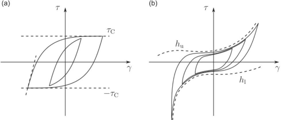
Recently, Al Majid and Dufour[9]introduced a Generalized Dahl Model (GDM) that allows the description of complex hysteresis shapes by including general envelope curves instead of constant asymptotes, as shown inFig. 8(b). Keeping the notations of Eq.(5), a simplified expression of the GDM can be written as follows:

d

τ

d

γ

¼

σ

τ

C h"

τ

sgnð _

γ

Þ ! "i (6) where h is an envelope function given by:

h ¼ðhuþ hlÞsgnð_

γ

Þ þ hð u" hlÞ

2 (7)

so that h describes the upper asymptote huwhen the strain rate _

γ

is positive and the lower asymptote hlwhen _

γ

is negative.

When h ¼

τ

C, the SFM is obtained. The constant i is taken equal to 1 by most authors[10,17].

This formulation is very general and has been used to describe various damping phenomena occurring in all-metal isolators[10], elastomers[18], belt tensioners[17,19]or rubber mounts[20]for example. However, its generality also leads to challenges in its application to complex hysteresis modelling. In particular, identification relies on the assumption of h expression, which can be polynomial[17,20], but can also include exponential terms or dependency with respect to the harmonic amplitude[10]or other parameters such as temperature.

Fig. 8. Hysteresis loops as can be described by (a) Dahl's Solid Friction Model (SFM)[16]with constant asymptotes τCand " τCand (b) the Generalized Dahl

Model (GDM)[9]with asymptotes huand hl.

4.1. A three-part hysteresis model

In the present work, the expression for h will be obtained from other hysteresis models. Based on the preliminary analysis of the measured loops inSection 3.2, the proposed model will be based on three parts, as illustrated in

Fig. 9:

#

Dahl's Dynamic Hysteresis Model[21]will be used to represent the classical dry-friction behaviour.

#

A polynomial term will account for the linear part and the stiffening behaviour.

#

A new formulation of the Bliman–Sorine model[22]will be used to include overshoot.

4.1.1. Part (a): Dahl's dynamic hysteresis model

Dahl's SFM (Eq.(5)) could be used to describe the dry friction hysteresis observed at low amplitudes (for

γ

0r5 ! 10" 3).

However, this model lacks nonlocal memory: its expression does not include information on the stress or strain at last change in the direction of the strain. The error arising from the lack of nonlocal memory when modelling non-harmonic response is illustrated inFig. 10(a): F denotes the point that should be reached and F’ the point that is actually reached. Moreover, even when modelling harmonic behaviour, this model leads to hysteresis loops with an initial slope depending on amplitude, which is undesirable. These limitations were addressed by Dahl in subsequent work, leading to a lesser known model, the Dynamic Hysteresis Model (DHM)[21], which principle is shown inFig. 10(b).

The DHM is based on the Prandtl rules[21]:

#

The slope of any hysteresis branch immediately after a velocity reversal is the same for all branches.

#

The shape of a branch depends only on the last point of velocity reversal.

#

When a branch goes through the last but one point of velocity reversal, the current loop is closed, and the branch continues as if this loop had never been formed. This is true both when closing a minor loop to return on the major loop, and when exceeding the maximum of the current major loop.

Fig. 9. Parts of the hysteresis loops used in the model decomposition: (a) dry friction hysteresis, (b) linear part and stiffening, and (c) overshoot.

Fig. 10. Non-harmonic response to the same excitation for both Dahl models: (a) Dahl's Solid Friction Model (SFM) and (b) Dahl's Dynamic Hysteresis Model (DHM), with branch index k in grey.

The last point corresponds to a fundamental property of hysteresis models with nonlocal memory called the wiping-out property[12,23]. This rule states that cycles with larger amplitudes wipe out the history of cycles with smaller amplitudes. Experimentally, it is indeed observed that the shape of major hysteresis loops does not depend on whether minor loops are formed or not, in a large range of fields including material plasticity[24], piezoelectric controllers[21]and friction[12]. It is also the case of the present hysteresis loops.

For stress–strain loops, the DHM links the restoring stress

τ

DHM _{with the strain}

_γ

_{and strain rate _}

_γ

_{by the following}

relationship: d

τ

DHM d

γ

¼

σ

2"

τ

DHM_"

_τ

mðkÞ

τ

C # $ sgn _! "

γ

# $i (8) The difference between the DHM and the SFM lies in the introduction of the term

τ

mðkÞ, which accounts for the stress at last velocity reversal point, k being the index of the current branch. This allows any branch of the hysteresis to start with the same initial slope 2

σ

after a velocity reversal. Vector

τ

mand index k are updated in the following way, as illustrated in

Fig. 10(b):

#

_{at first loading, k¼1 and}

τ

mð1Þ ¼ "

τ

Csgn _uð Þ (example: branch A - B inFig. 10(b));

#

at any strain direction reversal point, a new branch is created, k is increased by 1 and

τ

mðkÞ takes the value of

τ

at the

reversal point (branches B - C, C - D and D - C);

#

if a previous branch is crossed with k4 2, an internal loop is closed, the last two reversal points are “forgotten”, k is decreased by 2 (branch C - E);

#

if the current branch exceeds maximal load encountered previously, then all history is forgotten and the branch becomes a first loading branch with k¼1 and

τ

mð1Þ ¼ "

τ

Csgn _! " (branch E

γ

- F).

The two last points implement the memory wipe-out described above. In the following, parameter k is omitted for clarity.

The DHM can be seen as a particular case of the GDM presented in Eq.(6), with the following asymptote function: hDHM

τ

m; _

γ

! "

¼ 2

τ

Cþ

τ

msgn _! "

γ

(9)

It must be pointed out that the actual expressions of the asymptotes do not change from the SFM to the DHM, which means that hDHMis related but not equal to the expressions of the asymptotes:

hDHM

τ

m; _

γ

! " ¼

τ

C |{z} asymptotes ðSFMÞ þ

τ

Cþ

τ

msgn _! "

γ

|fflfflfflfflfflfflfflfflfflfflffl{zfflfflfflfflfflfflfflfflfflfflffl} nonlocal memory (10)

4.1.2. Part (b): including a polynomial term

In order to account for the linear part and the stiffening observed in the measurements, a polynomial term is included in the model:

τ

¼

τ

DHM_{þ Pð}

_γ

_{Þ (11)}

with

τ

DHM_{as defined in Eq.(8), and P a polynomial.}

Again, function h of the GDM can be written for the model including a polynomial. By differentiating Eq.(11)with respect to

γ

: d

τ

d

γ

¼

σ

τ

C 2

τ

C"

τ

DHM_"

_τ

DHM m ! _{"sgnð _}

γ

Þ ! " þ P0! "

γ

(12)

and writing

τ

DHM_¼

_τ

_{" Pð}

_γ

_{Þ leads to:}

d

τ

d

γ

¼

σ

τ

C 2

τ

Cþ P0_ð

_γ

_Þ

σ

=

τ

C"

τ

" Pð

γ

Þ "

τ

m" Pð

γ

mÞ ! " ! _{"sgn _}

γ

! " # $ (13) which corresponds to the GDM of Eq.(6)with

hpoly _

γ

;

γ

;

γ

m;

τ

m ! " ¼*

τ

Cþ Pð

γ

Þsgnð

γ

_Þ+ |fflfflfflfflfflfflfflfflfflfflfflfflfflffl{zfflfflfflfflfflfflfflfflfflfflfflfflfflffl} asymptotes ðSFMþpolynomialÞ þ P 0_ð

_γ

_Þ

σ

=

τ

C , -|fflfflfflffl{zfflfflfflffl} polynomial derivative þ*

τ

Cþ!

τ

m" Pð

γ

mÞ"sgnð _

γ

Þ+ |fflfflfflfflfflfflfflfflfflfflfflfflfflfflfflfflfflfflfflfflfflfflffl{zfflfflfflfflfflfflfflfflfflfflfflfflfflfflfflfflfflfflfflfflfflfflffl} nonlocal memory (14)

The three groups of terms in Eq.(14)show that the expressions of the asymptotes must be corrected with two terms to get the expression for h: first, a term proportional to the derivative of the polynomial, and secondly, a nonlocal memory

term. This is an important point to note if the identification of h is made from the asymptote curves, as prescribed by Al Majid[9].

4.2. Part (c): a new formulation of the Bliman–Sorine model

Hysteresis models that take into account an overshoot after the inversion in the strain direction include the LuGre (Lund– Grenoble) friction model[25]and the Bliman–Sorine model[22]. The Bliman–Sorine model being rate independent, it is chosen here as the observed behaviour does not depend on frequency.

As illustrated inFig. 11, the Bliman–Sorine model is defined as the sum of two Dahl models with different slope constants and asymptotic stresses of opposed signs:

d

τ

1 d

γ

¼

σ

1

τ

C1

τ

C1"

τ

1sgnð _

γ

Þ ! "

τ

1ð0Þ ¼ 0 ðaÞ d

τ

2 d

γ

¼

σ

2

τ

C2 "

τ

C2"

τ

2sgnð _

γ

Þ ! "

τ

2ð0Þ ¼ 0 ðbÞ

τ

¼

τ

1þ

τ

2 ðcÞ 8 > > > > > < > > > > > : (15)

where

τ

1and

τ

2represent two Dahl restoring stresses, with asymptotic stresses

τ

C1and "

τ

C2and initial slope

σ

1=

τ

C1and

σ

2=

τ

C2, respectively. The initial slopes are related by a factor

ξ

such that

σ

2=

τ

C2¼

ξ σ

! 1=

τ

C1" with 0r

ξ

r1. The same model

was introduced independently by Dahl some years later[26].

As discussed inSection 4.1.1, nonlocal memory is an important feature for hysteresis models to be applied to all types of excitations. The original Bliman–Sorine model is based on Dahl's original SFM[15], so it does not include nonlocal memory. The model is thus re-written here as a combination of two DHM rather than two SFM:

d

τ

1 d

γ

¼

σ

1

τ

C1 2

τ

C1"ð

τ

1"

τ

m1Þ ! sgn

γ

_ ! " ! " ðaÞ d

τ

2 d

γ

¼

ξσ

1

τ

C1 " 2

τ

C2"ð

τ

2"

τ

m2Þ ! sgn

γ

_ ! " ! " ðbÞ

τ

¼

τ

1þ

τ

2 ðcÞ 8 > > > > > < > > > > > : (16)

where

τ

m1and

τ

m2are the stresses at last inversion point for

τ

1and

τ

2respectively.

Apart from the original lack of nonlocal memory, one of the criticisms against the Bliman–Sorine model is the fact that it has two states, which can lead to numerical instabilities[27]. Here, a new one-state expression is derived fordτ

dγinstead of

the two state formulation. A one state formulation will be intrinsically more stable numerically than the original formulation.

Explicit expressions for

τ

2andddτγ2are obtained by first integrating and then re-deriving implicitEq. (16b)with respect

to

γ

:

τ

2¼

τ

m2" 2

τ

C2sgn _! "

γ

1 "exp "

ξσ

1

γ

"

γ

m 2 2 22

τ

C1 # $ # $ (17) d

τ

2 d

γ

¼ " 2

ξσ

1

τ

C2

τ

C1exp "

ξσ

1

τ

C1

γ

"

γ

m 2 2 22 # $ (18) where

γ

mis the shear strain at last inversion point.

By derivingEq. (16c) with respect to

γ

, inserting the implicit expression of dτ1

dγ Eq. (16a) and the explicit expression

ofdτ2

dγ Eq.(18), the following expression is obtained:

d

τ

d

γ

¼

σ

1

τ

C1 2

τ

C1"ð

τ

1"

τ

m1Þ ! sgn

γ

_ ! " ! " " 2

ξσ

1

τ

_τ

C2 C1exp "

ξσ

1

τ

C1

γ

"

γ

m 2 2 22 # $ (19) Then,

τ

1is replaced by

τ

"

τ

2,

τ

m1is replaced by

τ

m"

τ

m2, and

τ

2is replaced by its explicit expression from Eq.(17). After simplification, the final expression is:

d

τ

d

γ

¼

σ

1

τ

C1 2

τ

C1" 2

τ

C2 1" 1"

ξ

! _{"exp "}

ξσ

1

τ

C1

γ

"

γ

m 2 2 22 # $ # $ # "ð

τ

"

τ

mÞ ! sgn! ""

γ

_ (20) This expression follows the GDM expression of Eq.(6)with an asymptotic function hBSdefined by:

hBS _

γ

;

γ

;

γ

m;

τ

m ! " ¼ 2

τ

C1" 2

τ

C2 1" 1"!

ξ

"exp "

ξσ

1

τ

C1

γ

"

γ

m 2 2 22 # $ # $ þ

τ

m! sgn! "

γ

_ (21) This expression can be interpreted as follows. As

γ

tends to infinity, the asymptotic function tends towards 2ð

τ

C1"

τ

C2Þ þ

τ

m! sgn! ", which is the asymptotic function of a DHM with a constant asymptote

γ

_

τ

C1"

τ

C2, as shown in Eq.

(9). But immediately after a velocity reversal, the asymptotic function is equal to 2!

τ

C1"

ξτ

C2"þ

τ

m! sgn! ", which is larger,

γ

_ as 0r

ξ

r1 and

τ

C2o

τ

_C1. This higher asymptotic function allows the overshoot to occur. The asymptotic function then decreases exponentially from its value at velocity reversal to its value at infinity, which is consistent with the exponential decay observed in the Bliman–Sorine model due to the exponential behaviour of

τ

2(seeFig. 11).

4.3. Full hysteresis model

When taking into account dry friction hysteresis with nonlocal memory (part (a)), a polynomial term (part (b)) and an overshoot term (part (c)), the full expression for the model is:

d

τ

d

γ

¼

σ

1

τ

C1 h"

τ

sgnð _

γ

Þ ! " (22) with h _!

γ

;

γ

;

γ

m;

τ

m"¼ 2

τ

C1" 2

τ

C2 1" 1 "!

ξ

"exp "

ξσ

_τ

1 C1

γ

"

γ

m 2 2 22 # $ # $ þ P! "sgn _

γ

! "

γ

þ P 0_ð

_γ

_Þ

σ

1=

τ

C1þ

τ

m" P

γ

m ! " ! " ! sgn! "

γ

_ (23) As can be observed, a complex expression is obtained for h, which could not have been guessed directly from the hysteresis shape.

4.4. Model parameters and physical considerations

The general model is now adapted to the measured hysteresis loops in order to clarify the constant parameters that need to be identified for future simulations.

Polynomial: A simple polynomial expression is chosen to include the linear part of the loops as well as the observed stiffening behaviour:

P! "

γ

¼ G1

γ

þ G3

γ

3 (24)

where G1and G3are constant coefficients.

Overshoot: The effect of part (c) of the model should only be to add an overshoot to the dry friction loops of part (a). In particular, both the asymptotic stress and initial slope should remain unchanged when adding the overshoot. To this end,

τ

C1,

τ

C2 and

σ

1should be expressed with respect to the DHM parameters:

#

By definition of the Bliman–Sorine model, the final asymptote of the model is obtained by the difference between the two asymptotes (see Eqs. (16a)–(16c) andFig. 11). As

τ

Cis the asymptotic stress for the DHM, the relationship is the following:

τ

C1"

τ

C2¼

τ

C (25)

#

Writing the initial slopes for both models from Eqs.(8)and(20)allows expressing

σ

1as a function of

σ

: d

τ

d

γ

2 2 2 2_γ ¼γm ¼2

σ

1

τ

C1

τ

C1"

ξτ

C2 ! " ¼ 2

σ

(26)

which leads to:

σ

1¼

σ

τ

C1

Another element to take into account is the fact that the overshoot only appears at higher amplitudes in the experi-mental loops. In order to capture this behaviour,

τ

C2should depend on the amplitude. The type of amplitude dependency

has to be decided based on experimental observations. Both overshoot and stiffening were interpreted as a consequence of an increase in the number of contacts, as discussed inSection 3.2. In particular, the higher the amplitude, the more visible the stiffening, and the higher the overshoot. Thus, an hypothesis is made that the overshoot and the stiffening phenomenon are related. This is implemented by making

τ

C2proportional to the stiffening term at reversal point:

τ

C2ð

γ

mÞ ¼

α

G3

γ

3m (28)

where

α

is a constant to be determined.

From Eqs.(25),(27)and(28), it can be observed that

τ

C1and

σ

1will also depend on the amplitude:

τ

C1!

γ

m"¼

τ

Cþ

τ

C2!

γ

m" (29)

σ

1!

γ

m"¼

σ

τ

C

þ

τ

C2ð

γ

mÞ

τ

Cþ

τ

C2ð

γ

mÞ 1 "!

ξ

"

(30) Finally, the constant parameters to identify for the full model are the following:

#

the two DHM parameters

τ

C and

σ

;

#

two polynomial parameters: the “linear shear modulus” G1and the coefficient for the cubic term G3;

#

the two parameters for the overshoot model

ξ

and

α

¼

τ

C2ð

γ

mÞ=G3

γ

3m.

All the other parameters for the overshoot model,

τ

C2ð

γ

mÞ,

τ

C1!

γ

m" and

σ

1!

γ

m" can then be expressed from the previous

parameters.

5. Identification methods

In order to use the GDM, parameters are generally identified from the asymptotes of the hysteresis loops and their inner area[9,17]. However, this leads to two main issues:

#

First, as was shown inSections 4.1.1and4.1.2, the function h is related but not equal to the equation of the asymptotes, and identification must be carried out carefully by including correction terms.

#

Second, for complex shapes as encountered here, it is not trivial to obtain the asymptotes, as by definition the loops are not superposed or even close to the asymptotes except for high levels of deformation.

Here, the identification method relies on the decomposition of the model in three parts. In particular, a new identifi-cation method is developed for the DHM and extended to the addition of any polynomial term.

5.1. Identification of the DHM parameters

Instead of relying on the asymptote, the proposed identification method for the DHM relies on the backbone curve of the hysteresis loops (seeSection 3.2andFig. 12).

Eq.(8)is integrated to obtain the explicit expression of the stress for the DHM:

τ

DHM_¼

_τ

mþ 2

τ

C 1" e" σ τCjγ"γmj 3 4 sgn _! "

γ

(31)

Under a harmonic motion of amplitude

γ

0, the loops are comprised between a minimum point !

γ

min;

τ

min" and a

maximum point!

γ

max;

τ

max", with

γ

max¼

γ

0 and

γ

min¼ "

γ

0. The minimum and maximum points are the only reversal

points, and thus:

τ

m;

γ

m ! " ¼

τ

min;

γ

min ! " if sgn _! "

γ

40

τ

m;

γ

m ! " ¼

τ

max;

γ

max ! " if sgn _! "

γ

o0 ( (32) As the DHM is symmetrical and the motion is harmonic, the maximum and minimum are related as follows:

γ

min;

τ

min

! "

¼ "!

γ

max; "

τ

max" (33)

Moreover,

τ

maxis reached from

τ

minwhen sgnð _

γ

Þ 4 0, and

τ

minis reached from

τ

maxwhen sgnð _

γ

Þ o 0.

Inserting Eqs.(33)and(32)in Eq.(31), the following expression for the backbone curve is obtained:

τ

m¼ f_bbð

γ

mÞ (34) f_bbð

γ

Þ ¼

τ

C 1" e" 2 σ τCjγj 3 4 sgn! "

γ

(35)

with!

γ

m;

τ

m"¼

γ

min;

τ

min

! _{" or}

γ

_max;

τ

max

! _{". This expression contains all the parameters of the DHM, and allows a simple} identification from the minimum and maximum points of experimental loops measured at different amplitudes.

It can be noted that Eq.(31)can be obtained from Eq.(35)by replacing

τ

mbyð

τ

"

τ

mÞ=2 and

γ

mby!

γ

"

γ

m"=2. The DHM is

actually a specific case of the Masing rules[12], with an exponential backbone curve. 5.2. Extension to the DHM with a polynomial term

The backbone curve identification method presented in the previous section allows the inclusion of any polynomial term in the identification process without extra effort. Indeed, at a given loop extremum, adding the polynomial only shifts the stress by the polynomial value at this extremum:

τ

0

m¼

τ

mþ Pð

γ

mÞ.The expression of the backbone curve becomes:

f_bb! "

γ

¼

τ

C 1 "e" 2

σ τCj jγ

3 4

sgn! "

γ

þ P! "

γ

(36)

5.3. Identification method for the overshoot

The overshoot model parameters

ξ

and

α

can be identified in two different ways. As both Bliman and Sorine[22]and Dahl[26]proposed the same overshoot model separately, they also proposed their own identification procedures.Fig. 11

shows the five measurable values that are used by one or the other identification method:

# τ

1is the stress when strain approaches infinity:

τ

1¼ lim1

τ

¼

τ

C1"

τ

C2;

# τ

OSis the maximal stress reached at overshoot;

# γ

_OSis the shear strain for which

τ

OSis reached;

#

S is the initial slope: S ¼dτ

dγ

2 2 2_γ

¼ 0;

# γ

pis the strain for which the stress is within 5 percent of

τ

1.

Dahl[26]bases his identification method on S,

τ

OS,

γ

OSand

τ

1, while Bliman and Sorine[22]base theirs on

τ

OS,

γ

OS,

τ

1

and

γ

p. In the present case, as the initial slope is an important characteristic of the hysteresis loops related to the network

architecture, Dahl's identification procedure will be preferred. Moreover, parameter

γ

p can be hard to identify from

experimental loops where the decrease to the asymptote may not be a clean exponential decrease. The corresponding equations for Dahl's identification are presented inAppendix A.

6. Parameter identification and interpretation 6.1. Backbone curve identification of parts (a) and (b)

Parts (a) (Dahl's DHM) and (b) (polynomial term) of the model are first identified using the backbone curve method. The experimental backbone curve is defined from the extrema of the measured loops for all ten amplitudes from

γ

0¼ 5 ! 10" 4to

γ

0¼ 1 ! 10" 2, for the hysteresis loops measured at 20 Hz, as shown inFig. 13. The extrema are centred, with the hypothesis

that in this shear test the loops should be symmetrical. From Eqs.(24)and(36), the backbone curve expression is: f_bb! "

γ

¼

τ

C 1" e" 2

σ τ_Cj jγ

3 4

sgn! "

γ

þ G1

γ

þ G3

γ

3 (37)

The nonlinear least-square method is used to identify the parameters of this function from the ten experimental points, using MATLAB Curve Fitting Toolbox.Fig. 13shows a comparison between measured and simulated loops for parts (a) and (b) of the model, representing only the hysteresis without linear part

τ

" G1

γ

for legibility. Up to

γ

0¼ 5 ! 10" 4, the hysteresis

loops are well represented. For higher amplitudes, the overshoot phenomenon is clearly visible, which confirms the need for the third part of the model.

The parameters found for this set of samples at 20 Hz are:

τ

C¼ 1:07 ! 103Pa

σ

¼ 1:49 ! 106Pa

G1¼ 6:16 ! 106Pa G3¼ 2:38 ! 109Pa (38)

Fig. 13. Measured hysteresis loops for the first set of samples at 20 Hz (light grey full line), and corresponding backbone curve (black dashed line) and simulated hysteresis loops with parts (a) and (b) of the model α ¼ 0 and ξ ¼ 0 (dark grey full line). The removed linear modulus value is G1¼ 6:16 ! 106Pa.

Fig. 14. Measured hysteresis loops for the first set of samples at 20 Hz (light grey line) and simulated hysteresis loops with the full model including overshoot (dark grey line). The removed linear modulus value is G1¼ 6:16 ! 106Pa.

Fig. 15. Measured hysteresis loops for the second set of samples at 20 Hz (light grey line), and simulated hysteresis loops with the full model including overshoot (dark grey full line). The removed linear modulus value is G1¼ 5:91 ! 106Pa.

A new parameter is introduced: Gi¼ G1þ 2

σ

. This parameter corresponds to the initial slope of the hysteresis loops, and

thus to the modulus at very low amplitudes. From the values identified, Gi¼ 9:14 ! 106Pa. On the other hand, G1 corre-sponds to the asymptotic modulus, which is the modulus that would be reached at high amplitudes if there were no cubic term. Thus, the slope of the loop varies from Gito G1as the amplitude increases from a reversal point.

6.2. Identification of part (c) model parameters

The overshoot parameters

ξ

and

α

are now identified to be able to use the full model of Eqs.(22)and(23). Identification is carried out on the hysteresis loop of highest amplitude,

γ

0¼ 1 ! 10" 2. Parameters S,

τ

OS,

γ

OSand

τ

1(Fig. 11) are identified

successively on the superior ( _

γ

40) and inferior ( _

γ

o0) branches of the hysteresis loop. The obtained parameters are then

C 0 20 40 60 80 0 500 1000 1500 2000 (Pa) 0 20 40 60 80 0 1 2 3 4 5 6 7x 10 6 G 1 (Pa) 0 20 40 60 80 0 2 4 6 8 10x 10 6 G i (Pa) 0 20 40 60 80 0 0.5 1 1.5 2 2.5 3 3.5x 10 9 G 3 (Pa/m 2 ) 0 20 40 60 80 0 0.5 1 1.5 2 2.5 3 0 20 40 60 80 0 0.2 0.4 0.6 0.8

Set 1

Set 2

Frequency (Hz)

Frequency (Hz)

Frequency (Hz)

Frequency (Hz)

Frequency (Hz)

Frequency (Hz)

(f)

(e)

(a)

(b)

(c)

(d)

Fig. 16. Parameters for the two sets of samples: (a) asymptotic modulus, G1, (b) initial modulus Gi, (c) asymptotic stress τC, (d) cubic coefficient G3,

(e) overshoot parameter α and (f) overshoot parameter ξ. Parameters are identified on the backbone curve for ten amplitudes ranging from γ0¼ 5 ! 10" 4to

averaged to compensate for the asymmetry that could appear during measurement. Dahl's method(Appendix A)gives

ξ

and

τ

C2ð

γ

mÞ, from which

α

¼

τ

C2ð

γ

mÞ=G3

γ

3m is deduced.

The parameters found are:

α

¼ 0:92 ξ ¼ 0:37 (39)

Fig. 14shows the same experimental loops asFig. 13, compared with the full model. While there are still discrepancies between the model and experimental loops, the general behaviour is very well represented by the full model.

6.3. Variability and frequency dependency

A second set of samples was tested under the same conditions as the first set. Then, the identification procedure was applied to obtain the corresponding parameters for the model.Fig. 15shows the measured loops at 20 Hz as well as the simulated loops. Note that the linear modulus, removed from all figures, is slightly lower for the second set of samples, with G1¼ 5:91 ! 106Pa. Another difference that can be observed directly from the loops is that the samples of the second set

exhibit higher energy dissipation: the loops are more open than for the first set of samples.

Fig. 16shows a comparison between the identified parameters for both sets and for frequencies ranging from 1 Hz to 80 Hz.

It can be seen that the obtained values for the asymptotic and initial moduli G1and Giare very close for both sets and

have a very low frequency dependency, with slightly lower values for set 2. As the modulus evolves between Giand G1, it evolves roughly between 9 MPa and 6 MPa. While there has been no previous study on the shear behaviour of the material, a finite element analysis by Mezeix[28]indicated a shear modulus of 10 MPa. The order of magnitude is consistent with the present work.

Asymptotic stress

τ

C also has a low frequency dependency, but with a large difference between the two sets. This is

consistent with the fact that the loops measured for set 2 are more open that those measured for set 1. Parameter G3exhibits first a low difference between samples, which increases with frequency. This parameter is the only parameter of parts (a) and (b) that exhibits some frequency dependency: the parameter increases, which is consistent with the preliminary analysis inSection 3.2and with observations made by Janghorban on entangled fibres[29].

Finally, regarding parameters of the overshoot model (part (c)), a larger variation is observed both between samples and with frequency. This is due to the fact that the overshoot region in the loops is more subject to noise. The identification was not as efficient as for the other parameters, which indicates the need for a more robust identification process for this part. However, the obtained values still give the order of magnitude of those parameters.

This comparison between two sets of samples confirms the general behaviour observed for the first set of samples. The samples exhibit a low variability in modulus, but a higher variability in energy dissipation and stiffening behaviour. It is worth remembering that the samples are currently made manually. The good repeatability in modulus is a positive infor-mation, while the variability in energy dissipation indicates that more work is needed to understand and control better this fundamental property. The low frequency dependency of the material behaviour was also confirmed by parameter identification.

7. Conclusions

The shear behaviour of entangled cross-linked carbon fibres was studied at frequencies from 1 Hz to 80 Hz. Experimental testing of the material for amplitudes up to

γ

0¼ 1 ! 10" 2 showed a nonlinear behaviour with very low frequency

depen-dency. The analysis of the measured shear stress–strain hysteresis loops lead to a decomposition of the behaviour between a linear part and three nonlinear parts: a dry friction hysteresis (part (a)), a stiffening (part (b)) and an overshoot (part (c)), the two last parts appearing only at amplitudes higher than

γ

0¼ 5 ! 10" 3. The linear part was attributed to the stiffness of the

cross-linked contacts. Part (a) was attributed to fibres slipping against each other at free contacts. Parts (b) and (c) were assumed to come from the creation of new contacts between fibres at higher deformation amplitudes.

The hysteresis loops were modelled using Al Majid and Dufour's Generalized Dahl Model. Instead of assuming the expression of the asymptote function for this model, the three nonlinear parts of the behaviour were modelled separately before combining them. Dry friction was modelled using Dahl's lesser known Dynamic Hysteresis Model, and stiffening was included with a polynomial term. It was shown that the asymptote function in the Generalized Dahl Model is in fact related to but not equal to the actual asymptotes’ equations. A new one-state formulation for the Bliman–Sorine overshoot model was developed.

A new identification method was introduced for the Dynamic Hysteresis Model, relying on the backbone curve, and was extended to the addition of a polynomial term. The identification of the model parameters lead to a good capture of the hysteresis loops, showing the relevance of the developed model. Comparison between two sets of samples showed similar behaviours, but with some variability in the energy dissipation that could be analysed in further studies on the fabrication process of the material.

While the proposed combination of hysteresis models was applied to entangled cross-linked fibres in the present work, it could be used to model a large set of phenomena including friction, elasto-plasticity, stiffening, softening or stiction among

others. Other shapes could be modelled with the same model principle: asymmetrical loops can be achieved by using asymmetrical polynomials, or by defining different asymptotic functions for the upper and lower asymptotes.

Ongoing work will analyse the effect of the observed material behaviour on the vibratory response of a structure. The material model will be used in the analysis of both harmonic and transient nonlinear responses.

Acknowledgements

This study was carried out during the first author's PhD work at Institut Supérieur de l'Aéronautique et de l'Espace (ISAE) in Toulouse, France. Région Midi Pyrénée and Université de Toulouse are gratefully acknowledged for their financial support.

Appendix A. Dahl's identification method for the overshoot model The following parameters are defined from the parameters ofFig. 11:

d ¼

τ

C2

τ

1 ¼

τ

C2

τ

C1"

τ

C2 (A.1) c ¼1

ξ

(A.2) OS ¼

τ

OS

τ

1 (A.3) K ¼ S

γ

OS

τ

1 (A.4) In order to obtain c and d, the following system must be solved:

OS ¼ d þ1ð Þ c " 1ð Þexp " c c"1ln c þ c d 3 4 3 4 K ¼cþcd"d c"1 ln c þ c d 3 4 8 > > < > > : (A.5)

From c and d, the model parameters are obtained through the following relationships:

τ

C2¼ d $

τ

1

τ

C1¼

τ

1þ

τ

C2

ξ

¼1 c

σ

¼ c

τ

C1 c

τ

C1"

τ

C2S 8 > > > > > > > < > > > > > > > : (A.6) References

[1]C. Barbier, R. Dendievel, D. Rodney, Role of friction in the mechanics of nonbonded fibrous materials, Physical Review E 80 (1) (2009) 016115-1–5. [2]D. Poquillon, B. Viguier, E. Andrieu, Experimental data about mechanical behaviour during compression tests for various matted fibres, Journal of

Materials Science 40 (2005) 5963–5970.

[3]L. Mezeix, C. Bouvet, J. Huez, D. Poquillon, Mechanical behavior of entangled fibers and entangled cross-linked fibers during compression, Journal of Materials Science 44 (14) (2009) 3652–3661.

[4]L. Mezeix, D. Poquillon, C. Bouvet, Entangled cross-linked fibres for an application as core material for sandwich structures part I: experimental investigation, Applied Composite Materials (2015) 1–16.

[5]L. Mezeix, D. Poquillon, C. Bouvet, Entangled cross-linked fibres for an application as core material for sandwich structures – part II: analytical model, Applied Composite Materials (2015) 1–14.

[6]J.-P. Masse, D. Poquillon, Mechanical behavior of entangled materials with or without cross-linked fibers, Scripta Materialia 68 (2013) 39–43. [7]A. Shahdin, L. Mezeix, C. Bouvet, J. Morlier, Y. Gourinat, Fabrication and mechanical testing of glass fiber entangled sandwich beams: a comparison with

honeycomb and foam sandwich beams, Composite Structures 90 (2009) 404–412.

[8]T. Pritz, Frequency dependance of frame dynamic characteristics of mineral and glass wool materials, Journal of Sound and Vibration 106 (1986) 161–169.

[9]A. Al Majid, R. Dufour, Formulation of a hysteretic restoring force model. Application to vibration isolation, Nonlinear Dynamics 27 (2002) 69–85. [10]A. Al Majid, R. Dufour, Harmonic response of a structure mounted on an isolator modelled with a hysteretic operator: experiments and predictions,

Journal of Sound and Vibration 277 (2004) 391–403.

[11] D.J. Mead, A comparison of some equations for the flexural vibration of damped sandwich beams, Journal of Sound and Vibration 83 (1982) 363–377. [12]F. Al-Bender, W. Symens, J. Swevers, H. Van Brussel, Theoretical analysis of the dynamic behavior of hysteresis elements in mechanical systems, Journal

of Non-Linear Mechanics 39 (2004) 1721–1735.

[13]G. Muravskii, Application of hysteresis functions in vibration problems, Journal of Sound and Vibration 319 (2009) 476–490.

[14]M. Ismail, F. Ikhouane, J. Rodellar, The hysteresis Bouc–Wen model, a survey, Archives of Computational Methods in Engineering 16 (2009) 161–188. [15] P.R. Dahl, A Solid Friction Model, Technical Report, The Aerospace Corporation, May 1968.

[16]P.R. Dahl, Solid friction damping of mechanical vibrations, AIAA Journal 14 (12) (1976) 1675–1682.

[17] G. Michon, L. Manin, R. Dufour, Hysteretic behavior of a belt tensioner: modeling and experimental investigation, Journal of Vibration and Control 11 (9) (2005) 1147–1158.

[18]P. Saad, A. Al Majid, F. Thouverez, R. Dufour, Equivalent rheological and restoring force models for predicting the harmonic response of elastomer specimens, Journal of Sound and Vibration 290 (2006) 619–639.

[19] J. Bastien, G. Michon, L. Manin, R. Dufour, An analysis of the modified Dahl and Masing models: application to a belt tensioner, Journal of Sound and Vibration 302 (4–5) (2007) 841–864,http://dx.doi.org/10.1016/j.jsv.2006.12.013.

[20] B. Thomas, L. Manin, P. Goge, R. Dufour, A rubber mount model, Application to automotive equipment suspension, ISMA2010 International Conference on Noise and Vibration Engineering, Leuven, Belgium, 2010, 2010.

[21] P.R. Dahl, R. Wilder, Math model of hysteresis in piezo-electric actuators for precision pointing systems, Guidance and Control, 1985, pp. 61–88. [22] P.-A. Bliman, M. Sorine, Easy-to-use realistic dry friction models for automatic control, Proceedings of 3rd European Control Conference, 1995, pp. 3788–

3794.

[23] A. Visintin, Chapter 1 – Mathematical models of hysteresis, in: G. Bertotti, I.D. Mayergoyz (Eds.), The Science of Hysteresis, Academic Press, Oxford, 2006, pp. 1–123. ISBN 9780124808744,http://dx.doi.org/10.1016/B978-012480874-4/50004-X.

[24] P. Jayakumar, Modeling and Identification in Structural Dynamics, PhD Thesis, California Institute of Technology, 1987.

[25] C. Canudas de Wit, H. Olsson, K.J. Astrom, P. Lischinsky, A new model for control of systems with friction, IEEE Transactions on Automatic Control 40 (1995) 419–425.

[26] P.R. Dahl, Dynamic hysteresis model application to stiction type problems, Guidance and Control 2001, 2001, pp. 95–111.

[27] M. Gäfvert, Comparisons of two dynamic friction models, Proceedings of the 1997 IEEE International Conference on Control Applications, 1997, pp. 386– 391.

[28] L. Mezeix, Développement de matériaux d'âme pour structures sandwich à base de fibres enchevêtrées [Core Material Development for Sandwich Structures with Entangled Fibres], PhD Thesis, Université Paul Sabatier, Toulouse, 2010.

[29] A. Janghorban, D. Poquillon, B. Viguier, E. Andrieu, Compression de fibres enchevêtrées modèles [Compression of Calibrated Entangled Fibres], Matériaux 2006, Dijon, France, 2006.

[30] B. Borsotto, Modélisation, identification et commande d'un organe de friction. Application au contrôle d'un système d'embrayage et au filtrage d'acyclismes par glissement piloté [Modelling, Identification and Control of Friction System: Application to Clutch System Control and to Acyclisms Filtering by Sliding Control], PhD Thesis, Université Paris Sud-Paris XI, 2008.