Displacement Reconstructions in Ultrasound Elastography
Texte intégral
Figure
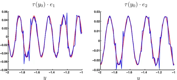
![Figure 6: Reconstructed displacement in both directions for different value of k ∈ [1/2, 3/2].](https://thumb-eu.123doks.com/thumbv2/123doknet/11642385.307339/19.918.172.732.78.334/figure-reconstructed-displacement-directions-different-value-k.webp)
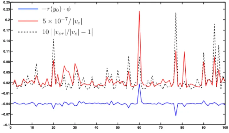
![Figure 8: Deviation of the ratio | v τ(l)ε /v ε | with respect to the gradient of the displacement to be reconstructed for different values of | k | ∈ [1/2, 3/2].](https://thumb-eu.123doks.com/thumbv2/123doknet/11642385.307339/20.918.272.610.202.447/figure-deviation-respect-gradient-displacement-reconstructed-different-values.webp)
Documents relatifs
Les modèles porcins d’hépatectomie et de transplantation de foie partiel ont été largement utilisés pour étudier les techniques chirurgicales de modulation du
Cette revue qui fera ultérieurement l’objet d’une publication est présentée en français, sous la forme d’un article (Résultats – Partie II – 2 – Les ARNlnc
Unfortunately, this is version 2.03 of OCamlP3l, way more evolved, and quite different from the version 0.9 used in the original research article, and there was no trace of the
[J1] Zhouye Chen, Adrian Basarab, and Denis Kouamé, ”Reconstruction of Enhanced Ultrasound Images From Compressed Measurements Using Simultaneous Direction Method of Multipliers,”
During imaging system investigation, the cavitation maps reconstruction achieved with different passive ultrasound techniques were assessed and the passive acoustic mapping
[r]
Since the gold nanoparticle solution has a surface plasmon resonance at 520 nm that is proportional to its concentration, the UV-Vis spectra obtained from the adsorption test could
community context. The opportunity for organizational expansion into housing development can be a catalyst to future economic development and community organizing... The
