Fatigue Crack Propagation Under Variable Amplitude Loading in Steels Used in Francis Turbine Runners

(1)

FATIGUE CRACK PROPAGATION UNDER VARIABLE AMPLITUDE LOADING IN STEELS USED IN FRANCIS TURBINE RUNNERS

MEYSAM HASSANIPOUR

DÉPARTEMENT DE GÉNIE MÉCANIQUE ÉCOLE POLYTECHNIQUE DE MONTRÉAL

THÈSE PRÉSENTÉE EN VUE DE L’OBTENTION DU DIPLÔME DE PHILOSOPHIAE DOCTOR

(GÉNIE MÉCANIQUE) OCTOBRE 2017

(2)

ÉCOLE POLYTECHNIQUE DE MONTRÉAL

Cette thèse intitulée :

FATIGUE CRACK PROPAGATION UNDER VARIABLE AMPLITUDE LOADING IN STEELS USED IN FRANCIS TURBINE RUNNERS

présentée par : HASSANIPOUR Meysam

en vue de l’obtention du diplôme de : Philosophiae Doctor a été dûment acceptée par le jury d’examen constitué de :

M. VADEAN Aurelian, Doctorat, président

M. TURENNE Sylvain, Ph. D., membre et directeur de recherche M. LANTEIGNE Jacques, Ph. D., membre et codirecteur de recherche Mme BROCHU Myriam, Ph. D., membre

(3)

DEDICATION

I hereby dedicate this thesis to everyone who contributes to

better understanding of the phenomena in this universe.

(4)

ACKNOWLEDGEMENTS

First of all, I would like to thank Yves Verreman, who is more than just a supervisor for me; He taught me how to conduct research, how to think, and how to express myself. He helped me to gain knowledge in this field and also contributed to my writing and speaking skills. I am grateful to have him as a supervisor and thankful for his great contribution to this thesis.

I would also like to thank senior researcher, Jacques Lanteigne, who co-supervised me and gave me access to the facilities at Institut de Recherche d’Hydro-Québec (IREQ), Hydro-Québec’s research center. Jianqiang Chen had a remarkable contribution in the beginning of this project and helped me to plan and develop the experimental program, so I am grateful to him for his help. I would like to thank Carlo Baillargeon who always found time to help me regarding problems that I encountered with the hydraulic machines during my 2-year experimental program at IREQ. I would also like to thank Stéphane Godin who supported me morally and scientifically while I was conducting my experiments. I am also thankful for the help and support I received from other researchers and technicians at IREQ.

I am grateful to the Natural Science and Engineering Research Council of Canada, Alstom Renewable Power Canada and Hydro-Québec Research Institute for their support.

Finally, I would like to thank my family who supported from a big distance. My dear friends Matjaz Panjan and Pierre Schell who put their time on reading and correcting some parts of this manuscript. I appreciate the help and encouragement of my beautiful friends in Montreal that kept me motivated during these 6 years. Thanks to my new friends here in Japan, especially Fransisca van Esterik and Ziane Izri, for their support and encouragement to reach the end of the line.

(5)

RÉSUMÉ

Les turbines hydrauliques sont soumises à de très grands nombres de cycles à faible amplitude de contrainte et à haute fréquence. Ces petits cycles sont générés par des phénomènes hydrauliques et sont superposés à une contrainte statique de tension. Aussi, dépendant des conditions de fonctionnement, il est possible d’avoir superposé aux petits cycles un plus faible nombre de grands cycles à forte amplitude de contrainte et basse fréquence. On a ainsi en pratique une superposition de petits cycles, de grands cycles et d’une contrainte statique de tension durant les 70 ans de durée de vie de la turbine.

Les turbines hydrauliques qui sont fabriquées à partir des aciers AISI 415, ASTM A516, et AISI 304L (notés 415, A516, et 304L pour simplification) sont soumises à de telles contraintes cycliques et statique. Ces contraintes ont pour effet de favoriser la propagation des défauts existants dans les roues des turbines et peuvent mener à leur rupture.

Pour éviter la propagation des fissures, les petits cycles doivent induire un ΔK qui est en dessous du seuil de fatigue. Néanmoins, les grands cycles peuvent contribuer à propager ces fissures. Ainsi, pour prédire la vitesse de propagation des fissures dans de telles conditions de cycles superposés, on a recours à la sommation linéaire de dommage (SLD). Il a été observé que les grands cycles superposés aux petits cycles peuvent induire une diminution du seuil de fatigue des petits cycles. Différentes procédures ont été proposées dans la littérature pour mesurer les seuils associés au petits cycles seuls et avec superposition des grands cycles. Cependant, la plupart des procédures ne minimise pas la fermeture induite lors de la mesure du seuil conduisant ainsi à une surestimation de leur valeur. La présente étude propose de nouvelles procédures d’essais pour réduire la fermeture lors de la mesure du seuil de fatigue pour les aciers mentionnés précédemment. De plus, différentes études ont démontré que les fissures peuvent se propager plus rapidement sous l’effet des grands cycles que ce que prédit la SLD. Nous vérifierons ainsi la précision de la prédiction LDS par rapport aux mesures de propagation.

Dans une première étude, la propagation des fissures par l’interaction de petits et de grands cycles est caractérisée dans les trois aciers. Les cycles de base sont entrecoupés par les grands cycles. Les vitesses de propagation des fissures par les cycles de base et les grands cycles de sous-charges sont additionnées dans la SLD pour évaluer la vitesse de propagation de fissure. Les mesures expérimentales de vitesse de propagation en sous-charges périodiques sont ensuite comparées avec

(6)

la prévision de la SLD. Le ratio entre la mesure de propagation de fissure et la prédiction SLD est définie comme facteur d’accélération.

Les résultats montrent que les mesures de propagation par les sous-charges périodiques dans l’acier 415 sont proches de celles déterminées par la méthode de SLD. Cependant, le facteur d’accélération est égal à trois dans l’acier 304L. Des valeurs intermédiaires sont obtenues pour l’acier A516. On montre que le facteur d’accélération est directement relié au coefficient d’écrouissage de chacun des aciers. En ordre croissant, l’acier 415 a le plus faible coefficient d’écrouissage, suivi par l’acier A516 et par l’acier 304L.

Les observations fractographiques montrent que la sous-charge cause une accélération de la propagation de fissure pendant les cycles de base. La cause de cette accélération est attribuée à une combinaison de contrainte résiduelle en tension et d’écrouissage causée par les sous-charges. Une deuxième étude avait pour but de mesurer le seuil de fatigue des petits cycles (cycles de base) et de vérifier comment il pouvait être diminué par la superposition de grands cycles (sous-charges périodiques). Les essais de fatigue de cette seconde étude ont été réalisés dans la région du seuil de propagation sur les aciers avec le plus petit et le plus grand facteur d’accélération, soit les aciers 415 et 304L respectivement.

Le ratio de nombre de cycles de base sur nombre de sous-charges est noté n. Deux procédures d’essais ont été realisés. Le premier a été realisé par une reduction de ΔK pour mesurer un seuil conventionnel, ΔKth,conv, de 2 × 10-7 mm/cycle en amplitude constante et avec les sous-charges périodiques avec différents n. Le deuxième procédure a été realisé par une croissance de ΔKBL de zero avec les sous-charge periodiques pour n = 1.25 × 103 _{pour atteindre un seuil réel, ΔK}

th,true, avec une vitesse de propagation de 6.7 × 10-9_{mm/cycle et ensuite ΔK}

th,conv.

Le seuil de fatigue des petits cycles ne décroît pas pour n > 1.25 × 105_{. Le nombre de petits cycles} est de l’ordre de 7 × 1010_{pendant une durée de vie de 70 ans. Le nombre de grands cycles ne doit} donc pas dépasser 5.6 × 105_{cycles. Lorsque n < 10}5_{, le seuil de fatigue commence à décroître.} Cette décroissance est moins importante dans le 415 que dans le 304L. Il a été démontré que le seuil de fatigue décroît 5 fois plus quand la vitesse de propagation est en dessous de 6.7 × 10-9 mm/cycle par rapport à 2 × 10-7_mm/cycle.

Les contraintes résiduelles de tension sont induites dans les roues lors de la fabrication et du soudage. Ces contraintes augmentent le facteur d’intensité de contrainte maximal, Kmax, induit aux défauts et peuvent favoriser la propagation des fissures. L’effet d’une augmentation de Kmax sur le

(7)

seuil de fatigue en amplitude constante et sous-charges périodiques doit être étudiée. Il a été démontré qu’une augmentation de Kmax décroît légèrement les deux seuils.

(8)

ABSTRACT

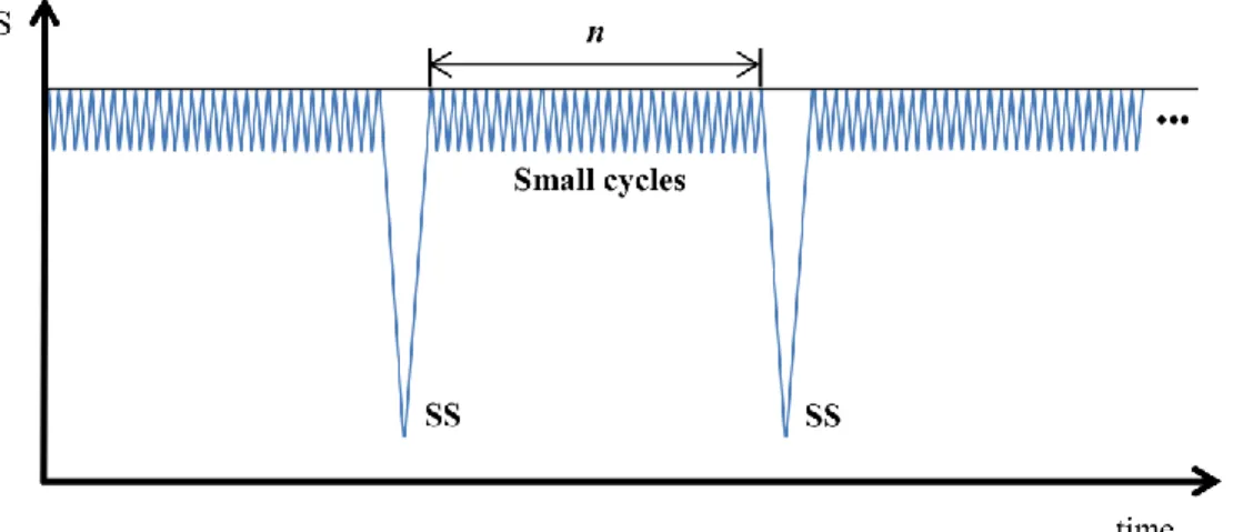
Hydraulic turbine runners are subjected to a very large number of cycles with small stress amplitudes at high frequencies. These cycles are generated by hydraulic phenomena and are superimposed to a tensile static stress. Depending on the operating conditions, much lower number of large cycles are generated with large stress amplitudes at low frequencies. As a summary, the whole stress spectrum consists of small cycles superimposed to a tensile static stress that is intercut with large cycles during the 70 years design life of turbine runners.

Turbine runners, which are fabricated from AISI 415, ASTM A516, and AISI 304L steels (i.e. called 415, A516 and 304L for simplicity), are subjected to the aforementioned stress cycles. The imposed stress spectrum propagates the existing defects or cracks in turbine runners and may lead to their failure.

In order to avoid crack propagation, the small cycles should induce a ΔK that is lower than the fatigue threshold. Nonetheless, the crack can grow due to large cycles. As a result, linear damage summation (LDS) is employed to predict the crack growth. The large cycles superimposed to small cycles can also induce a decrease in fatigue threshold of the small cycles.

Different test procedures have been proposed to measure the fatigue threshold of small cycles and the ones superimposed to large cycles; however, most of them do not minimize the crack closure while reaching the fatigue threshold leading to an overestimation of fatigue thresholds. In this study new test procedures are proposed in order to minimize crack closure while reaching the fatigue thresholds in turbine runner steels. Different studies have shown that crack can grow faster than the LDS prediction due to the interaction between large cycles. Therefore, we verify the precision of LDS prediction compared to the measured crack growth rates.

In this first study, crack growth due to the interaction between two large cycles is investigated in the three aforementioned turbine runner steels. Baseline cycles are periodically intercut by an underload cycle. This variable amplitude loading is hereafter called periodic underloads. Crack growth rates of baseline cycles and underload cycles are summated in LDS to predict crack growth under periodic underloads. Crack growth measured under periodic underloads is then compared to LDS prediction. A ratio between the measured and predicted crack growth, that is greater than unity, is defined as an acceleration factor.

Results show that the measured crack growths under periodic underloads in the 415 steel are close to the ones predicted by LDS. On the other hand, the acceleration factor in the 304L steel can reach

(9)

up to three. Intermediate values are obtained for the A516 steel. We show that there is a direction relationship between the strain hardening exponent and the acceleration factors in each steel. In increasing order, the 415 steel has the lowest monotonic strain hardening exponent, followed by A516 and 304L steels.

The fractography analysis showed that an underload followed by baseline cycles causes an increase in crack growth during baseline cycles, which leads to acceleration factors. It is presumed that an underload induces a combination of tensile residual stress and strain hardening that increase crack growth during subsequent baseline cycles.

In the second study, the aim is to measure the fatigue threshold of small cycles (baseline cycles) and to verify its reduction due to large cycles (periodic underloads) are called periodic underloads.. Given that these tests in this region are time-consuming, fatigue tests were only conducted on steels with the lowest and highest acceleration factors in the first study; thus, the 415 and 304L steels, respectively.

The ratio of the number of baseline cycles over number of periodic underloads is defined as n. Two load procedures were conducted to investigate the effect of underloads on the baseline cycles. A first load procedure was conducted with decreasing ΔK to measure a conventional fatigue threshold, ΔKth,conv, at a crack growth rate of 2 × 10-7 mm/cycle under constant amplitude loading and under periodic underloads at different n ratios. Then a second load procedure was conducted with increasing ΔKBL from zero to measured ΔKth,true at a crack growth rate of 6.7 × 10-9 mm/cycle and ΔKth,conv under periodic underloads at n = 1.25 × 103.

The fatigue threshold of small cycles does not decrease for n > 1.25 × 105_._{In turbine runners, the} number of small cycles during 70 years of design life (about 7 × 1010_{). In order to avoid a decrease} in the fatigue threshold, the number of large cycles (periodic underloads) should be kept below 5.6 × 105_{. The fatigue threshold of small cycles starts to decrease for n < 1.25 × 10}5_{. This decrease} is lower for the 415 steel as compared to 304L. The decrease in fatigue threshold due to periodic underloads is about five times higher when it is measured at 6.7 × 10-9_mm/cycle.

Tensile residual stress is induced in turbine runners during the fabrication and welding procedure. This stress increases the tensile static stress in runners, which leads to an increase in the Kmax at the defect tip. As a result, the effect of an increase in the Kmax on crack growth under constant and periodic underloads was also investigated. It is revealed that an increase in the Kmax slightly decreases the fatigue threshold under constant and under periodic underloads.

(10)

LIST OF TABLES

Table 6.1 Typical load pattern for a Francis turbine runner [1] ... 61

Table 6.2 Chemical compositions of studied materials (wt. %) ... 64

Table 6.3 Average prior austenite grain size on the three orthogonal planes of each steel (μm) .. 66

Table 6.4 Tensile properties of the three wrought steels in L and T directions at room temperature ... 67

Table 6.5 Maximum SIF at the tip of initial defects corresponding to runner lifetimes of 20 and 70 years ... 68

Table 6.6 Loading parameters for POV and SS sequences ... 68

Table 6.7 Parameters of Walker equation for each steel ... 73

Table 6.8 Maximum acceleration factors for the three steels at both Kmax and n ... 75

Table 6.9 Comparison of measured crack growth with different prediction methods for the three steels (acceleration factors are calculated at Kmax,70, Ψ = 0.33 and n = 10) ... 77

Table 8.1 Comparison of tensile properties in the old and new A516 steel with ASTM A516...106

Table 8.2 Comparison of acceleration factors in the old and new A516 steels at n = 3 and 10 at Kmax = 19.44 MPa.m1/2 ... 107

(14)

LIST OF FIGURES

Figure 1.1 Hydraulic Francis turbine and runner components ... 1

Figure 2.1 Different periods of fatigue life [14]...7

Figure 2.2 Slips bands under a) monotonous load, and b) cyclic load [11] ... 8

Figure 2.3 Stress intensity factor at the tip of a sharp crack in an infinite plane [14] ... 10

Figure 2.4 a) Three load modes of fatigue crack in a specimen, and b) monotonous plastic zones for each load mode under plane stress and plane stress using the Von Mises yield criterion [21]...11

Figure 2.5 Crack growth rates versus ΔK in three different regions (adapted from [34]) ... 13

Figure 2.6 Two different procedures to measure the fatigue threshold, a) constant R ratio (ASTM standard), b) constant Kmax [32, 37]... 15

Figure 2.7 Crack growth rates versus ΔKeff in the three different crack propagation regions [25, 31] ... 16

Figure 2.8 a) Variation in plastic zone throughout the thickness, and b) variations in Kcl at three different ΔK due to a decrease in thickness in an 7075-T6 aluminum alloy specimen [21, 49] .... 17

Figure 2.9 a) Surface asperities in the crack wake in an 2090-T8E41 aluminum lithium alloy, b) variations in Kcl at three different ΔK due to removal of the crack wake asperities in an 7075-T6 aluminum alloy specimen [21, 49] ... 18

Figure 2.10 Schematic illustration of a zigzag crack path to estimate the Kcl [59, 60]... 18

Figure 2.11 Crack closure mechanisms at different crack growth regions at R = 0.05 [29] ... 20

Figure 2.12 Schematic of load and crack opening displacement measured from crack mouth clip gauges behind the crack tip ... 21

Figure 2.13 Test procedures to determine the SIF corresponding to the crack propagation, a) at low R ratios, b) at high R ratios [93-94] ... 22

Figure 2.14 Crack growth after an applied overload, a) crack growth rate as a function of crack length, b) crack length as a function of number of cycles [108] ... 27

Figure 2.15 Crack growth rates as a function of crack length after an applied overload and compressive underloads in austenitic stainless steel 316L [118] ... 28

(15)

Figure 2.16 Schematic of crack closure variation after an applied overload and underload at

different crack growth regions (adapted from [123]) ... 29

Figure 2.17 Two prediction models, a) Wheeler, and b) Willenborg (adapted from [144]) ... 33

Figure 2.18 Prediction of the crack growth rate following a single overload [148] ... 35

Figure 2.19 Example of CORPUS crack closure model in a simplified spectrum [151] ... 36

Figure 3.1 a) Different regions of a runner blade based on stress magnitude [154], and b) steel plate filled with epoxy and silicone to protect strain gauges installed on region A of a runner blade [4]...38

Figure 3.2 Typical stress spectrum imposed on turbine runners with small cycles superimposed to the highest tensile static stress, a) small cycles with low stress amplitudes, and b) small cycles with high stress amplitudes (adapted from [155, 156]) ... 39

Figure 3.3 a) Linear damage summation employed to predict initial defect dimensions that will not cause rupture for 70 years, b) initial allowable semi-elliptical defect dimensions in different regions of a blade runner ... 40

Figure 3.4 Simplified load spectrum with POVs and SS sequences ... 42

Figure 3.5 Simplified load spectrum with small cycles and SS sequences ... 43

Figure 3.6 Compact tension specimen installed in an Instron servo-hydraulic machine ... 46

Figure 5.1 Crack growth rates versus ΔK and ΔKeff at R = 0.1 in the 415 and 304L steels……..53

Figure 5.2 Comparison of crack growth rates at R = 0.1 and 0.7 in the 415 steel ... 54

Figure 5.3 Comparison of crack growth rates at R = 0.1 and 0.7 in the 304L steel ... 54

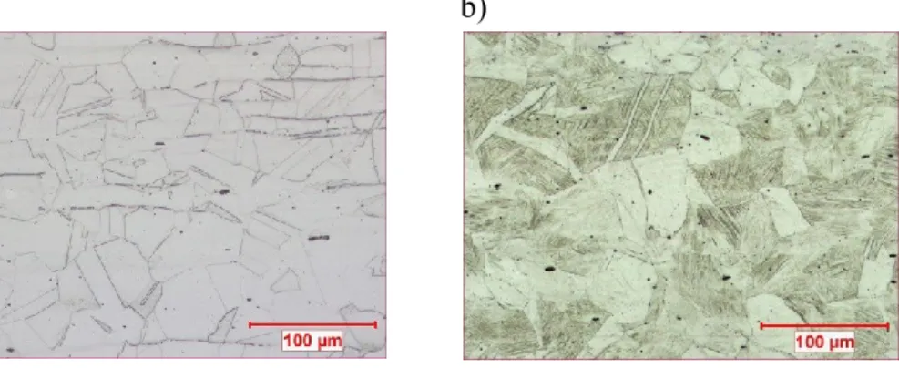
Figure 5.4 Microstructure of the 304L in the LS orientation, a) as received, b) close to the necking of the tensile specimen (L direction) ... 55

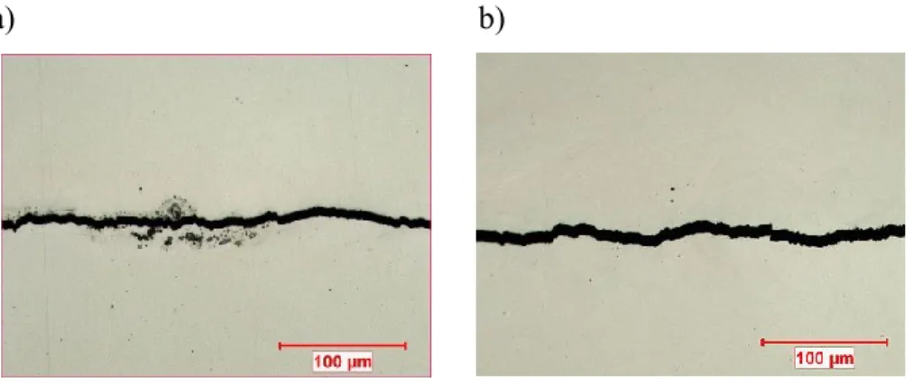
Figure 5.5 Crack path on the surface of the specimen at ΔKth,conv in the 415 steel at, a) R = 0.1, and b) R = 0.7 ... 56

Figure 5.6 Crack path on the surface of the specimen at ΔKth,conv in the 304L steel at, a) R = 0.1, and b) R = 0.7 ... 56

Figure 6. 1 Different load cycles under variable amplitude loading...62

(16)

Figure 6.3 Applied loading sequence on the three steels at constant Kmax, ... 69 Figure 6.4 Schematic of crack deflection angle (θ) and crack deflection length (l) ... 70 Figure 6.5 Crack path deflection under constant amplitude loading at Kmax,70 and R = 0.1 in the a) 415 steel, b) A516 steel, and c) 304L steel (crack propagates from left to right in the three cases) ... 71 Figure 6.6 Crack growth rates versus load ratio and corresponding Walker predictions at Kmax,70 ... 72 Figure 6.7 Crack growth rates versus load ratio and corresponding Walker predictions at Kmax,20 ... 72 Figure 6.8 Fatigue striations on fatigue surfaces under constant amplitude loading at Kmax,20, (a) 415 steel at R = 0.1, (b) A516 steel at R = 0.1, c) 304L steel at R = 0.1, and d) 304L steel at R = 0.7 (crack propagates from left to right in all cases) ... 74 Figure 6.9 Acceleration factors for the three steels at Kmax,70 and n = 10 (curves are obtained from a third order polynomial regression of the data) ... 76 Figure 6.10 Acceleration factors for the three steels at Kmax,20 and n = 10 (curves are obtained from a third order polynomial regression of the data) ... 76 Figure 6.11 Striations on fatigue surfaces in the 304L steel at Kmax,20 under periodic underloads (RBL = 0.7, RUL = 0.1 and n =10). Figure 5.11 (b) is an enlargement of Figure 5.11 (a) (the crack propagates from left to right in all cases) ... 79 Figure 7.1 Two different load procedures to measure the fatigue threshold at high R ratio, (a) constant R ratio (ASTM standard), (b) constant Kmax [37]...86 Figure 7.2 Step-by-step decreasing Kmax load procedure to measure the fatigue threshold at

constant high R ratio under PUL (adapted from [128]) ... 87 Figure 7.3 Effect of n ratio on the fatigue threshold at high R ratio of an 2024-T351 aluminum alloy under periodic underloads (PUL) and periodic compressive underloads (PCUL) (adapted from [128]) ... 88 Figure 7.4 Constant Kmax procedure to measure the fatigue threshold at high R ratio under PUL (adapted from [132]) ... 88 Figure 7.5 Kmax effect on the fatigue threshold under CAL and PUL (adapted from [132]) ... 89

(17)

Figure 7.6 Microstructure of the two wrought steels: (a) 415 steel, and (b) 304L steel ... 90 Figure 7.7 Load sequences in the first load procedure with decreasing ΔK under CAL and PUL at a given n ratio ... 92 Figure 7.8 Expected results of load procedure in Figure 7.7 in a da/dN – ΔKBL plot ... 92 Figure 7.9 Load sequences in the second load procedure with increasing ΔKBL under PUL (n = 103_{) ... 94} Figure 7.10 Expected results of load procedure in Figure 7.9 in a da/dN – ΔKBL plot ... 94 Figure 7.11 Log-linear plot of crack growth rates versus SIF range of baseline cycles under CAL and PUL at different n ratios in the 415 steel ... 96 Figure 7.12 Log-linear plot of crack growth rates versus SIF range of baseline cycles under CAL and PUL at different n ratios in the 304L steel ... 96 Figure 7.13 Decrease in ΔKth,conv due to periodic underloads in both steels ... 97 Figure 7.14 Effect of periodic underloads at n = 103_{on ΔK}

th,conv and ΔKth,true of the 415 steel in a log-linear da/dN – ΔKBL plot ... 99 Figure 7.15 Effect of periodic underloads at n = 103_{on ΔK}

th,conv and ΔKth,true of the 304L steel in a log-linear da/dN – ΔKBL plot ... 99 Figure 8.1 Effect of Kmax on crack growth rates at high R ratios in the 415 steel...104 Figure 8.2 Effect of Kmax on crack growth rates at high R ratios in the 304L steel ... 105 Figure 8.3 Log-linear of da/dN versus ΔKBL curve under CAL and PUL in the 415 and the 304L steels at n = 102_{... 109} Figure 8.4 Crack growth rates versus linear ΔKBL from different test procedures under CAL and PUL in 415 steel ... 111 Figure 8.5 Crack growth rates versus linear ΔKBL from different test procedures under CAL and PUL in 304L steel ... 111 Figure 9.1 Startup and SNL in an operating turbine runner with a repeated sequence...113 Figure 9.2 Stress spectrum with three stress cycles imposed at the defect tip ... 114

(18)

LIST OF SYMBOLS AND ABBREVIATIONS

Latin symbols

a and c length and width of semi-elliptical defect

a20 maximum initial crack length allowed for 20 years design life a70 maximum initial crack length allowed for 70 years design life b and t runner blade length and thickness

b’ _{Basquin equation exponent}

c’ _{Coffin-Manson equation exponent}

CR0 and p Walker equation parameters

F and Q geometric functions for calculating stress intensity factor

H strength coefficient

Kmax,OL maximum stress intensity factor of an overload

Kt stress concentration factor

Kmax,th maximum stress intensity factor range at the fatigue threshold

Kmax,1 maximum stress intensity factor of 11.11 MPa.m1/2

Kmax,2 maximum stress intensity factor of 19.43 MPa.m1/2

l crack length deflection

m Paris equation exponent

n frequency of baseline cycles over underload cycles, ΔNBL/ΔNUL q number of underload cycles in one block

R stress ratio

RBL load ratio of baseline cycles RUL load ratio of underload cycles

ry,OL monotonous plastic zone size created by an overload

(19)

ryc cyclic plastic zone size

ryc′ cyclic plastic zone size of an underload cycle

s strain hardening exponent

W compact tension specimen width

Greek symbols

Δablock crack growth in one load block

ΔK stress intensity factor range

ΔKeff effective SIF range

ΔKBL stress intensity factor range of baseline cycles

ΔKth stress intensity factor range at the fatigue threshold

ΔKth,eff effective stress intensity factor range at the fatigue threshold ΔKth,conv conventional fatigue threshold (2 × 10-7 mm/cycle)

ΔKth,true true fatigue threshold (6.7 × 10-9 mm/cycle)

ΔKth,CAL true fatigue threshold under constant amplitude loading

ΔKUL stress intensity factor range of an underload

ΔNBL number of baseline cycles in one load block

ΔNUL number of underload cycles in one load block

δUL underload cycle striation width δBL baseline cycle striation width

ε true strain

εe elastic strain

εf true strain at fracture

εp plastic strain

εr relative elongation at rupture

(20)

σ true stress

σij stress components

σf true stress at fracture

φ angle of a specific point at the front of a semi-elliptical defect Ψ ratio of stress intensity factor ranges, ΔKBL/ΔKUL

Abbreviations

BL baseline cycles

CAL constant amplitude loading

CT compact tension specimen

COD crack opening displacement

L longitudinal (rolling) direction of the plate

LT long transverse orientation

LS long-short transverse orientation

LDS linear damage summation

OL single overload

POV power output variations

PUL periodic underloads

S short-transverse direction of the plate

SS start/stop sequences

SIF stress intensity factor

T transverse direction of the plate TS transverse-short transverse orientation

(21)

CHAPTER 1 INTRODUCTION

1.1 Context

Hydraulic turbines are the main sources of electricity generation from hydro energy. This energy is renewable, non-polluting, and more efficient than the one generated by fossil fuels [1]. A hydraulic Francis turbine and its components are shown in Figure 1.1. In this type of turbine, water enters a spiral casing in a radial direction with respect to a shaft. It is then directed inside a runner by the circumferential wicket gates [1]. It hits the runner blades successively and leaves a torque on the runner. This torque induces a spin in the runner, which is coupled to a rotor by the shaft. When the rotor spins inside the magnetic field of a stator, electricity is generated.

Figure 1.1 Hydraulic Francis turbine and runner components

The water flow creates a tensile static stress on the blade. This stress leaves a torque that induces a spin in the runner with respect to the shaft. As the blade moves forward, the induced stress gradually decreases; however, the subsequent wicket gate directs the water to hit the blade and re-increase the stress to its maximum. So the blade continues to move forward [2]. These repeated sequences, known as wicket gates and blade interactions, and other hydraulic phenomena create stress fluctuations on the blade which vary from maximum to minimum values [3]. These small pressure

Wicket gates Rotor Spiral casing Turbine runner Blades and crown Blades and band Stator

(22)

fluctuations create cycles with small stress amplitudes that are superimposed to the tensile static stress.

During an initial period, where the runner is not coupled to the rotor, the wicket gates are partially opened and direct the water flow to spin the runner. This flow generates an initial startup and spin-no-load in the stress spectrum. Subsequently, to generate electricity, the runner becomes coupled to the rotor and the wicket gates become completely open. As a result, the tensile static stress increases to a maximum level.

During the runner operation, electricity demands vary and cause variations in the electricity production known as power output variations. These variations are adjusted by pivoting the wicket gates that control the water flow. By completely closing the wicket gates, the static stress induced on the runner blades is reduced to zero, so that the runner stops spinning. These start/stop sequences are repeated throughout the design life of the runner. In some cases, a sudden uncoupling between the rotor and runner may occur [4]. As a result, the runner does not transfer the torque to the rotor. This causes the runner to spin at a higher speed (overspeed) till the wicket gates stop the water flowing into the runner. This is known as load rejection or overspeed [4, 5]. The aforementioned changes in the operating conditions create cycles with large stress amplitude, which intercut the tensile static stress.

As a summary, on one hand, interaction between the wicket gates and blade plus other hydraulic phenomena creates small stress amplitude cycles in the runner. On the other hand, power output variations, start/stop sequences, and load rejections create large stress amplitude cycles in the runner. Therefore, the runner is subjected to small stress amplitude cycles that are superimposed to tensile static stress, which is intercut with large stress amplitude cycles in the stress spectrum. For convenience, we refer to the aforementioned stress cycles as small and large cycles, hereafter.

(23)

1.2 Problematics

Runners are mostly fabricated from cast steels. A martensitic stainless steel, ASTM CA6NM, has recently been used to fabricate the turbine runners. The ASTM A36, a ferritic-pearlitic cast steel, was used to fabricate many runners which are installed in Hydro-Quebec power stations. Some other runners are fabricated from the ASTM CF8, a cast austenitic stainless steel. Runners may also be fabricated using the wrought version of the aforementioned steels, which are the AISI 415, ASTM 516, and 304L steels, respectively. In this study, the wrought steels are chosen in order to have less dispersion in the results.

Defects are formed during the fabrication process (i.e. casting and welding) or the operation (i.e. cavitation) of runners. Defects or cracks in high stress regions of the blade propagate due to small cycles superimposed to a tensile static stress intercut with large cycles.

In some power stations with recently built runners, the stress amplitude of small cycles is low (few MPa) and induces a ΔK that is below the crack propagation threshold. As a result, they do not induce crack growths and can be neglected; however, large cycles generated by operating conditions can grow the defects in the runner and can lead to its failure within 70 years of design life.

In the engineering approach, linear damage summation (LDS) is employed to predict defect growth due to large stress amplitude cycles. Thus, using the LDS prediction method, during the operation runners are periodically stopped to inspect and verify defect growth as compared to the one predicted by LDS; however, stopping runners for an inspection decreases energy production, which is a costly procedure. Thus, there is a tendency to rely on crack growth predicted by LDS and minimize inspections or carry them out when it is necessary.

In reality, however, interaction between large cycles can increase defect growth in runners. Consequently, defects will grow faster than the one predicted by LDS and may lead to the failure of the runners before a scheduled inspection. As a result, there is a need for a precise crack growth prediction that will enable designers to minimize the frequency of inspections.

In some power stations with aged runners, the stress amplitude of small cycles is high (tens of MPa) and induces a ΔK that is close to the fatigue threshold. The hydraulic phenomena generate a large number of small cycles during the life design of the runners. Therefore, the ΔK at the defect tips will be below the fatigue threshold. Otherwise, small cycles will propagate the defects, which

(24)

lead to an early failure of runners. Large cycles can further decrease the fatigue threshold of small cycles and lead to the propagation of defects. Thus, the fatigue threshold of small cycles and the one intercut with large should be measured.

Tensile residual stresses are induced in the runners during the fabrication and welding process. As the crack propagates in the runner it can be subjected to these tensile residual stresses, which will increase the tensile static stress at the defect tip. Higher tensile static stress may decrease the fatigue threshold of small cycles. Moreover, higher tensile static stress may decrease the fatigue threshold of small cycles intercut with periodic underloads.

1.3 Research objectives

In a first study, small cycles induce a ΔK that is below the fatigue threshold. So they do not cause crack propagation. Thus, the cycles are neglected in the load spectrum and the effect of large cycles on crack growth is investigated. Crack growths measured under large cycles will be compared to the ones predicted using linear damage summation.

In a second study, small cycles induce a ΔK that is close to the fatigue threshold. So the crack can grow and may lead to runner’s premature failure. Thus, the fatigue threshold of small cycles will be measured. Moreover, large cycles can decrease the fatigue threshold of small cycles. Thus, the decrease in the fatigue threshold of small cycles due to large cycles will be defined.

A higher tensile static stress may induce a decrease in the fatigue threshold of small cycles and the ones intercut with large cycles. Therefore, the decrease in both fatigue thresholds due to higher tensile static stress will be defined.

Specific objectives

Crack growth under constant amplitude loading in the three different steels at different R ratios will be investigated. Factors that may affect crack growth at different R ratios will also be investigated.

Different load procedures proposed in literature will be studied, and a procedure leading to better estimation of load interaction between load cycles and more accurate measurement of ΔKth will be conducted. Fatigue testing with two different amplitude cycles (small and large) in a load spectrum will be developed and implemented.

(25)

Accuracy of LDS prediction is verified for each steel, and factors leading to an increase in crack growth due to small and large cycles will be analyzed. The effect of large cycles on the fatigue threshold of small cycles measured with low and very low crack growth rate will be investigated.

1.4 Outline of the thesis

The second chapter is a literature review on fatigue. The fatigue initiation that may lead to propagation is shortly summarized. A review of different studies on fatigue crack propagation under constant amplitude loading and variable amplitude loading is then presented. Finally, factors influencing crack propagation and the suggested prediction methods are presented.

The third chapter explains the methodology that was chosen to carry out the studies and conduct fatigue tests. The microstructural characterization and tensile test are then explained in detail. The fourth chapter, exaplins about the following chapter and the organization of the whole

The fifth chapter presents the fatigue tests conducted under constant amplitude loading. The results of this chapter are employed in chapter 6.

The sixth chapter presents the fatigue tests conducted according to the first study and the corresponding results. This chapter is presented as a published article.

The seventh chapter presents the fatigue tests conducted according to the second study and the corresponding results. This chapter is presented as a published article.

The eighth chapter is a general discussion on the studies conducted in the previous chapters. Crack growth rates under constant amplitude loading and periodic underloads are discussed.

The final chapter covers the main conclusion and proposes to study a real and non-simplified stress spectrum in runners.

(26)

CHAPTER 2 LITERATURE REVIEW

2.1 Brief historical review

During the first industrial revolution, most structures were made of steels that could be loaded under a high tensile load [6]. Steels were widely used in the railroad industry. In the design, stress applied on steels was limited to monotonous yield stress while taking into account a safety factor; however, regular failures were reported on railroad axles made of steels [7]. These failures implied that cyclic stresses below the yield stress can induce local deformation in the railroad axles leading to their failure. This was a first incident implying the importance of considering cyclic stresses and loads in design.

During the Second World War, failure occurred in a large number of ships that were made of steels and whose hulls were welded. In 2003, in Quebec, at the Sainte-Marguerite 3 power station, many defects grew during the operation of the Francis turbine runners, which were made of steels. This problem caused a huge reduction in the production of electricity [8]. Thus, different incidents such as those mentioned above have implied that more investigations should be conducted on the effect of the cyclic stresses on steels in order to improve their design in structures.

The term fatigue is defined as “ the process of progressive localized permanent structural change occurring in a material subjected to conditions which produce fluctuating stresses and strains at some points and which may culminate in cracks or complete fracture after a sufficient number of fluctuations [9].” Two major approaches in structural fatigue design employed to conduct fatigue tests in materials will be presented.

2.2 Approaches in structural fatigue design

2.2.1 Total life approach

In the total life approach, a laboratory specimen is usually subjected to a cyclic nominal stress amplitude (ΔS) or cyclic local strain amplitude (Δε) until it fails [10]. Different levels of cyclic stress or strain are applied as a function of the number of cycles until the failure occurs, which are known as the ΔS-N or Δε-N curves. High amplitude of the stress or strain will result in failure with a low number of cycles, or low cycle fatigue. Otherwise, this is known as high cycle fatigue [11].

(27)

A real structure can be designed based on the aforementioned curves for a high or low number of cycles; however, a small defect free laboratory specimen subjected to ΔS under stress will endure more cycles as compared to the real structure with defects [12]. Thus, in this case, the estimated fatigue life will be longer and the design approach is non-conservative; however, as the specimen becomes similar to the real structure, the design becomes realistic.

2.2.2 Defect tolerant approach

In this approach, a structure is considered to have defects. So, an initial crack length, which represents the defect, is generated in the laboratory specimen under nominal stress or strain [13]. The crack growth rates in materials are measured in the specimen. Then using the measured crack growth rates and Fracture Mechanics concepts, the initial defect dimensions that will not lead to the structure’s failure during their design life is estimated.

2.3 Fatigue life

Figure 2.1 shows the different periods of fatigue life for any structure subjected to fluctuating stresses and strains. The fatigue life is divided into a nucleation period followed by a crack growth period until reaching the final failure. After the crack nucleation, a microcrack or short crack starts to grow. The local stress and strain distributions in front of the crack tip may arrest the growth of the short crack. Otherwise, it grows and becomes a macrocrack or long crack. This long crack may propagate until the final failure.

(28)

2.3.1 Crack nucleation

In crystalline materials such as steels, there are inherent defects in crystals called dislocations. Plastic deformation results from the dislocation movements in high atomic density planes, called slip planes [11]. When a steel specimen is monotonically loaded, local slip bands resembling to a staircase are formed on the specimen surface, as shown in Figure 2.2a [11]. When a specimen is loaded cyclically, the density of slip lines or bands increases and accumulates on the surface. These slip bands create some intrusions and extrusions on the surface as shown in Figure 2.2b. This leads to the crack nucleation after a certain number of cycles.

a) b)

Figure 2.2 Slips bands under a) monotonous load, and b) cyclic load [11]

The relation between the nominal stress amplitude (ΔS) and number of cycles (N) to failure is given by the Basquin equation:

 

b f S σ=  N 

 (2.1)

where σ’f is approximately equal to the true stress at fracture, σf, and b′ is a fitting exponent. The relation between the local strain amplitude (Δε) and number of cycles to failure is given by the Coffin-Manson equation:

 

b

 

c f f σ N N E =



 



    (2.2)

where E is Young’s Modulus, ε’f is approximately equal to the true strain at fracture, εf , and c′ is a fitting exponent. Both correlations were found for uniaxial stress or strain at an R ratio (minimum load over the maximum one) equal to -1. Other studies proposed a correlation between the stress or strain at different R ratios with the number of cycles to failure [15]. In the case where nucleation

(29)

does not occur for a specified high number of cycles (e.g. 107_{cycles), it is assumed that the fatigue} limit is reached and the specimen will not fail [16].

It was, however, observed that the specimen fails at a stress below the fatigue limit with a number of cycles that is higher than 107 _{[17]. In this case, it is observed that nucleation occurs below the} surface from an inclusion or void in the steel [17].

2.3.2 Short crack growth

After that crack nucleates, it is still small or short and may continue to grow [18]. The cracks is

microstructurally small if its length is comparable to the length of the microstructure, for example,

a crack smaller than the grain size [19]. It is mechanically small if its length is small as compared to the local plastic deformation, for example, a crack growing out of a notch [20]. It is physically

small if its length is small, for example, a length typically between 0.1 and 1 mm. A short crack

must overcome microstructural barriers and the local plastic strain at its tip to propagate and become a macro crack, and leading to complete failure.

2.3.3 Long crack growth

Once the crack has overcome microstructural barriers and the plastic deformation at its tip, it becomes physically long. At this stage, the crack grows in a continuum medium. As it grows, the crack tip plasticity becomes negligible as compared to the crack length and specimen geometry [16]. Thus, the specimen is considered to be nominally elastic and plasticity is only limited to the crack tip. These conditions are called small scale yielding [21].

a) Stress intensity factor

Stress intensity factor is a parameter that characterizes the elastic field in the vicinity of a sharp crack tip under small scale yielding conditions. Structures in the linear elastic continuum mechanics must satisfy equilibrium and compatibility equations. The Airy stress function (φ) satisfies both equations which are combined in one equation called the bi-harmonic [22].

A singular stress field is created in the vicinity of a sharp crack. A complex stress function was proposed to satisfy bi-harmonic equations for singular stress fields [21]. This function was first proposed for a sharp crack under a bi-axial stress in an infinite plate. However, it was modified later for a uni-axial tensile stress, which results to the definition of a stress intensity factor (K) [23], which is given by following equation:

(30)

I

K = S 2πa

where S is the nominal applied stress, and 2a is the crack length in the infinite plate shown in Figure 2.3. Later a geometric function, Y, was used to define a corresponding K in a finite plate.

Figure 2.3 Stress intensity factor at the tip of a sharp crack in an infinite plane [14] b) Load modes and plasticity

As shown in Figure 2.4a, crack may grow due to three different loads with respect to its plane. If the load opens the crack planes, it is called mode I. If it shears the crack planes, it is called mode II; and if it twists the tip of the crack plane, it is called mode III [24, 25].

σ12

σ11

(31)

Figure 2.4

a) Three load modes of fatigue crack in a specimen, and b) monotonous plastic zones for each load mode under plane stress and plane stress using the Von Mises yield criterion [21] Local stress components (σij) at a given distance (r) and angle (θ) from the crack tip (see Figure 2.3) are correlated to K for all three load modes by the following equation.

 

I II III ij ij ij ij K K K σ f θ + g θ + h θ 2πr 2πr 2πr = (2.3)

The fij(θ), gij(θ), hij(θ) are trigonometric functions [22]. The aforementioned equation terms can have a second higher order term [26], known as the T stress, but it is not considered here. Stress components close to the crack tip (r tends towards zero) increase towards infinity; however, plasticity at the crack tip limits stress components to the yield stress of the material. Three dimensional stress components are usually simplified into two dimensional ones, under a plane stress or plane strain state. Inserting stress components into the von Mises yield criterion gives an equivalent stress that is compared to the yield stress of the steel. The two dimensional stress components in Equation 2.3 are inserted into von Mises criterion to derive the boundary of the plastic zone size [21]. These boundaries for the three load modes are shown in Figure 2.4b. The size of the monotonous plastic boundary or zone, ry, for Mode I and θ = 0, can be written as:

(32)

max         2 y ys K 1 r = απ σ (2.4)

where Kmax is the maximum stress intensity factor (SIF), σys is the yield stress of the steel, and the value of α depends on the stress state at the crack tip. The value of α is estimated by two different approaches for the plane stress state [27].Both approaches results in roughly similar values, where α is equal to 1 [21, 22]. The value of α increases to 3 for the plane strain state due to stress triaxiality at the crack tip.

On the other hand, the size of the cyclic plastic zone, ry is given as:

         2 yc yc 1 ΔK r = π σ (2.5)

where ΔK is the SIF range (Kmax - Kmin), σyc is the cyclic yield stress of the steel, and the value of β depends on the cyclic stress at the crack tip. Some studies estimated that β is equal to 4α for a quasi-stationary crack. Thus, the cyclic plastic zone size is estimated to be roughly one-fourth of the monotonous one [28]; however, other studies suggested that the cyclic plastic zone may be one-fourth to one-tenth of the monotonous one for a growing crack [29, 30].

2.4. Crack growth under constant amplitude loading

2.4.1 Crack growth regions

Fatigue crack growth rates as a function of SIF range, ΔK, in steels consists of three distinct regions, as shown in Figure 2.5 [31]. Most of the fatigue test procedures in literature were first conducted in the medium crack growth rates region, known as Paris [31]. Later, many tests were conducted in the low crack growth rates region, known as near-threshold. Thus, we first introduce the Paris region and then the near-threshold region.

a) Paris region

After a conventional pre-cracking, the initial ΔK and Kmax are gradually increased at a constant R ratio to measure crack growth rates. The shape and the amount of the increasing gradient dKmax/da do not affect crack growth rates [32]. A correlation between crack growth rates (da/dN) and SIF range, ΔK, was found in region II [33]. This correlation is given by the following equation;

(33)



Δ



m

da

C K

dN 

Δ

K



K

max



K

min (2.6)

which is known as the Paris equation and where c and m are the steel or material parameters. Crack growth rates versus ΔK are measured using a laboratory specimen to obtain Paris equation parameters. In real structures, ΔK is calculated by estimating a geometric factor (Y), the applied load range and a typical crack length (ao) [21, 22]. Next, crack growth in each step (Δai) is calculated at a given ΔK using Paris equation parameters for a number of cycles. Finally, the total crack growth is incremented step-by-step to predict crack growth in the structure as shown in Equation 2.7.



Δ



, 0

  m   

i i i

a C K N a a a (2.7)

Crack growth rates are high in Region III. Thus, a given crack length is reached with much fewer cycles as compared to the Paris region. Crack growth is quasi-static within this region, and when the maximum SIF reaches the critical SIF, catastrophic failure occurs.

(34)

b) Fatigue threshold region

After a conventional pre-cracking, the initial ΔK and Kmax parameter should be decreased at a constant R ratio following a specific procedure to reach a ΔK that will not induce crack growth, known as the fatigue threshold; however, a high decreasing gradient of the aforementioned parameter builds up a higher amount of plasticity and roughness in the crack wake, which can close the crack while reaching the fatigue threshold [25]. This can underestimate the crack growth rate at a given ΔK in the near-threshold region and overestimate the fatigue threshold [32]. Consequently, different test procedures are proposed in literature to minimize extra crack closure, while reaching the fatigue threshold.

An early test procedure was conducted by keeping the maximum displacement constant as the crack length increases during the test; however, this procedure induces a constant and low decreasing gradient, dKmax/da. Consequently, this test procedure is time consuming. Afterwards, it was proposed to decrease Kmax step-by-step but by imposing some limit conditions on the decrease in Kmax [32]. However, these conditions do not minimize the crack closure at the near-threshold region. Finally, a procedure known as the ASTM E647 was proposed to conduct a continuous decrease in the Kmax and limit the decreasing gradient of dKmax/da in order for it not to be higher than 0.08 mm-1 _{(Figure 2.6).}

That being said, even low dKmax/da can induce extra crack closure [35]. Thus, in order to eliminate the consequences of dKmax/da, some studies proposed a constant Kmax procedure where only ΔK was decreased to reach ΔKth (Figure 2.6). This procedure minimizes extra crack closure induced in the crack wake [36]. The aforementioned test procedures are explained in detail in Chapter 7.

(35)

a) b)

Figure 2.6 Two different procedures to measure the fatigue threshold, a) constant R ratio (ASTM standard), b) constant Kmax [32, 37]

The near-threshold region is sensitive to the microstructure [21]. The beginning of this region corresponds to a crack growth rate that may vary from 10-8 _{to 10}-7 _{mm/cycle, and the corresponding} ΔK is the so-called fatigue threshold (ΔKth) [38]. The SIF at the crack tip below the ΔKth value is assumed to not cause any crack propagation [34]. The end of region I is estimated to be close to 10-6_{mm/cycle for steels, which is close to a lattice spacing per cycle [31, 39].}

2.4.2 Crack closure

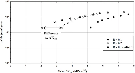
As the R ratio increases, the crack growth rate versus ΔK increases in the Paris region as shown in Figure 2.5. Crack growth rates further increase in the near threshold region and lead to a lower fatigue threshold, ΔKth, at a high R ratio as compared to a low R ratio [40-42].

It was reported that during the unloading, the crack may close at a SIF, Kcl above Kmin at low R ratios. On the other hand, during the loading, the crack opens at a SIF, Kop, above Kmin. The SIF at closure (Kcl) and opening (Kop) are close to each other [30]. It was concluded that crack grows only when the opening part of ΔK is applied. Thus, Kcl is deducted from Kmax to calculate the opening part of ΔK, known as the effective SIF range, ΔKeff, and is given in Equation 2.8.



,



,



,



min

ΔK_eff K_{m x}_a K_c_l R K K_cl R K K (2.8)

At a given Kmax, as R ratio increases, Kmin increases until it becomes equal to or higher than Kcl. As a result, ΔKeff becomes equal to ΔK. The estimated crack growth rate as a function of ΔKeff at different R ratios is given by the following equation,

(36)



Δ _eff





Δ _eff



m

da

f K C K

dN   (2.9)

results in similar crack growth rates and gives a constant ΔKth. Therefore, crack growth rates at different R ratios can be shown as a single curve as a function of ΔKeff as shown in Figure 2.7.

Figure 2.7 Crack growth rates versus ΔKeff in the three different crack propagation regions [25, 31]

a) Crack closure in different crack growth rates regions

It was reported that plasticity induces compressive residual stress in the crack wake, which leads to crack closure in the Paris region [43]. This assumption was validated with compliance measurements and fractographic evidence [44, 45]; however, fatigue tests in the near-threshold region revealed that other factors can also induce crack closure [46, 47].

Plasticity is higher on the surface of the specimen as compared to the center of it [48], as shown in Figure 2.8a. Removing material at the surface of the specimen around the crack and decreasing its thickness lead to a decrease in the estimated crack closure level at higher ΔK values (8.8 and 17.6 MPa.m1/2_{) in the Paris region in an 7075-T6 aluminum alloy. Crack closure level reaches a constant} value at certain thickness as shown in Figure 2.8b [49]; however, crack closure level remains constant throughout the thickness at the lowest ΔK value (2.5 MPa.m1/2_{) corresponding to the} near-threshold region as shown in Figure 2.8b. Thus, it was concluded that plasticity induces crack

(37)

closure (plasticity-induced crack closure) mainly on the surface of the specimen (crack flanks) and is higher in the Paris region than in the near-threshold region.

The plastic deformation left in the crack flanks transforms the austenite to martensite in some steels [50, 51]. The austenite phase in steels has a face centered cubic crystal structure. A sufficient amount of deformation transforms the face centered cubic crystals to the body centered tetragonal crystals, which is the martensitic phase [52-55]. It has been shown that this transformation leads to a decrease of ductility at the crack tip and increases crack growth rates in the Paris region. On the other hand, this transformation induces volume expansion in crack flanks, which induces crack closure in the near-threshold region [51, 54, 56, 57].

a) b)

Figure 2.8 a) Variation in plastic zone throughout the thickness, and b) variations in Kcl at three different ΔK due to a decrease in thickness in an 7075-T6 aluminum alloy specimen [21, 49] On the other hand, as the crack grows and deflects from its straight path, it leaves some asperities in the crack wake [58]. A deflected crack under nominal load mode I becomes locally under load modes I and II, so both the tensile and sliding displacement occur [59]. A combination of the crack wake asperities and sliding displacement under mode II creates a mismatch in the crack wake, as shown in Figure 2.9a in an 2090-T8E41 aluminum lithium alloy [60]. This mismatch creates a contact point in the crack wake and makes the crack close before reaching the minimum load, inducing crack closure (roughness-induced crack closure) [61, 62].

(38)

a) b)

Figure 2.9 a) Surface asperities in the crack wake in an 2090-T8E41 aluminum lithium alloy, b) variations in Kcl at three different ΔK due to removal of the crack wake asperities in an 7075-T6

aluminum alloy specimen [21, 49]

Removal of crack wake asperities at the lowest ΔK (2.5 MPa.m1/2_{) value in the near-threshold} region decreased the crack closure level, as shown in Figure 2.9b [49]; however, this wake removal did not affect crack closure levels at higher ΔK values in the Paris region. Thus, it was concluded that surface asperities induce a higher crack closure in the near-threshold region than in the Paris region.

One study suggested that the stress intensity factor (K) for a deflected crack under modes I and II (kI and kII)can be estimated by considering the crack angle deflection, θ, which is shown in Figure 2.10.

Figure 2.10 Schematic illustration of a zigzag crack path to estimate the Kcl [59, 60] Thus, an equation was proposed to calculate k1 and k2 at the crack tip as followed [11]:

3 2

cos ( / 2)



, sin( / 2)cos ( / 2)



 

I I II I

k K k K (2.10)

(39)

The kI and kII at the crack tip are lower than KI. The equivalent effective SIF range at the crack tip can be estimated using the maximum energy release rate theory [6]:



₂ ₂



1/2

 

eff I II

k k k (2.11)

The above equation leads to an effective SIF range (ΔKeff) of a deflected crack. This range over SIF in load mode I (ΔKI) for a straight crack leads to the following equation:

1/2

6 2 4

1

/ cos sin cos

2 2 2



           _ _{ }_ _{ } _{ }__          eff U k K (2.12)

Another study suggested that the crack closure can be estimated from surface asperities in the crack wake with the following equation (adapted from [58, 59]):

1 2 1 1 1 2



   __  __  _  _ x U R x (2.13)

where x is equal to the displacement induced by load mode II over load mode I (x =uII/uI), and γ is equal to the height of an irregularity (h) over the crack length deflection from the straight path (w), (γ = h/w), as shown in Figure 2.10.

Another type of crack closure can be induced by oxidation in the crack wake. This closure occurs in steels sensitive to oxidation, where the environment can interact with a slow growing crack in the near-threshold region [31, 63].

The Kop/Kmax is shown for three different alloys at R = 0.05 in Figure 2.11. As the ΔK decreases towards low ΔK values in the near-threshold region, crack closure levels increase [29]. Crack closure is mainly induced by surface asperities and oxide at low ΔK. On the other hand, it is mainly induced by plasticity and phase transformation at high ΔK, as shown in Figure 2.11.

(40)

Figure 2.11 Crack closure mechanisms at different crack growth regions at R = 0.05 [29]

b) Errors in crack closure estimation

The SIF at crack closure, Kcl, is conventionally estimated from the point where a deviation occurs in the linear load-COD curve; this method is suggested by the ASTM E647 [64]. A first contact induced by plasticity and/or surface asperities in the crack wake creates the aforementioned deviation in the load-COD curve, which corresponds to the load at crack closure, Pcl (Figure 2.12). Using the Pcl to estimate the ΔKeff leads to crack growth rates that are equal at all R ratios. This was conventionally accepted in the literature [25, 65]; however, some new studies have found that the Kcl estimated using the ASTM E647 method, leads to a ΔKeff at low R ratios that is lower than the one at high R ratios [66]. Therefore, different studies were conducted to explain the difference in Kcl and ΔKeff at low and high R ratios [43, 67-73].

Some studies stated that as the crack wake behind the crack tip is in contact locally, the crack tip can still be in tension [74, 75]. On the other hand, as the load gradually decreases to a minimum load (Pmin), the dP/dCOD gradually increases until it becomes equal to the one corresponding to the dPmin/dCODmin. Therefore, there is a gradual decrease in the Pcl point until it reaches the Pmin. This gradual decrease makes it difficult to define a Pcl point in the load-COD curve.

(41)

Figure 2.12 Schematic of load and crack opening displacement measured from crack mouth clip gauges behind the crack tip

As a result, different methods are proposed to estimate Pcl point in the P-COD curve [76-79]. Some studies proposed the intersection between the linear dP/dCOD at the maximum load (Pmax) and the minimum load should define the Pcl on the load-COD curve (see Pcl,1 in Figure 2.12) [80, 81]. Other studies suggested that the intersection between the dP/dCOD at Pmax and the one corresponding to a completely closed crack at dPmin/dCODmin should define the Pcl on the load-COD curve (see Pcl,2 in Figure 2.12) [79, 82, 83]. A review of the different estimation methods can be found in [72, 82, 84].

Crack closure at low R ratios is detected using global measurements, but this is not the case at high R ratios; however, it was shown in a recent study that local measurements (strain gauges) near the crack tip at low and high R ratios using the ASTM method lead to a unique ΔKeff at all R ratios [85].

Different studies have reported a wide dispersion in the crack closure estimations [36, 86]. For example, two tests were conducted using the same test procedure and measurement technique on two Astroloy nickel based alloys; however, the estimated crack closure levels were different while reaching the fatigue threshold [86]. Heterogeneity in the material causes random distribution of surface asperities in the crack wake, which leads to a variation in crack closure [87]. Other studies have shown that as the geometry, location, and number of asperities in the crack wake vary, the crack closure level also varies [87-89]. Therefore, they concluded that the crack closure cannot be used to estimate the ΔKeff [82, 90, 91].

(42)

Since it is difficult to determine the Kcl in the load-COD curve, a new test procedure was developed to determine crack closure at the crack tip at low and high R. This method suggests that the crack propagates when the there is a transition in the local stresses from the compression to tension at the crack tip [92]. In this procedure, the crack is loaded at an initial ΔK and it is increased step-by-step, as shown in Figure 2.13a at low R ratios and in Figure 2.13b at high R ratios, until the crack starts to grow. The SIF corresponding to the crack propagation, Kpr, is defined as the average between the Kmax without crack growth and the one with crack growth. As a result, the effective SIF or ΔK that makes the crack grow is defined as follows, ΔKeff = Kmax – Kpr (R), so Kpr is only a function of the R ratio [93]. It has been shown that the ΔKeff estimated using this method at low R ratios is equal to the one measured at high R ratios using the ASTM method and constant Kmax procedure [94].

a) b)

Figure 2.13 Test procedures to determine the SIF corresponding to the crack propagation, a) at low R ratios, b) at high R ratios [93-94]

Fatigue Crack Propagation Under Variable Amplitude Loading in Steels Used in Francis Turbine Runners

DEDICATION

ACKNOWLEDGEMENTS

RÉSUMÉ

ABSTRACT

TABLE OF CONTENTS

LIST OF TABLES

LIST OF FIGURES

LIST OF SYMBOLS AND ABBREVIATIONS

CHAPTER 1 INTRODUCTION

1.1 Context

1.2 Problematics

1.3 Research objectives

1.4 Outline of the thesis

CHAPTER 2 LITERATURE REVIEW

2.1 Brief historical review

2.2 Approaches in structural fatigue design

2.3 Fatigue life

 

 

 





 

 

 

2.4. Crack growth under constant amplitude loading





Δ

K



K



K







































