A Comprehensive Review of Vertical Ground Heat Exchangers Sizing Models With Suggested Improvements

(1)

UNIVERSITÉ DE MONTRÉAL

A COMPREHENSIVE REVIEW OF VERTICAL GROUND HEAT EXCHANGERS SIZING MODELS WITH SUGGESTED IMPROVEMENTS

MOHAMMADAMIN AHMADFARD DÉPARTEMENT DE GÉNIE MÉCANIQUE ÉCOLE POLYTECHNIQUE DE MONTRÉAL

THÈSE PRÉSENTÉE EN VUE DE L’OBTENTION DU DIPLÔME DE PHILOSOPHIAE DOCTOR

(GÉNIE MÉCANIQUE) AVRIL 2018

(2)

UNIVERSITÉ DE MONTRÉAL

ÉCOLE POLYTECHNIQUE DE MONTRÉAL

Cette thèse intitulée :

A COMPREHENSIVE REVIEW OF VERTICAL GROUND HEAT EXCHANGERS SIZING MODELS WITH SUGGESTED IMPROVEMENTS

présentée par : AHMADFARD Mohammadamin

en vue de l’obtention du diplôme de : Philosophiae Doctor a été dûment acceptée par le jury d’examen constitué de :

M. CIMMINO Massimo, Ph. D., président

M. BERNIER Michel, Ph. D., membre et directeur de recherche M. KUMMERT Michaël, Ph. D., membre

(3)

DEDICATION

(4)

ACKNOWLEDGEMENTS

This thesis is the results of four years of efforts that would certainly have been impossible to accomplish without the help and support of the people I met during my doctoral career.

To begin, I would like to thank my research supervisor, Professor Michel Bernier for his advice and support on this project. His words of encouragements and knowledge positively affected this research and his valuable words will follow me throughout all my life.

I would like to acknowledge the support of Professors Kummert and Pasquier who helped me to learn many things and to thank Professors Lamarche and Cimmino who accepted to be members of the jury.

Throughout these years, I enjoyed the company of Massimo, Vivien; Nicolas, Bruno, Patricia,

Pauline, Laurent, Corentin, Adam and Houaida, my student colleagues of the Building and

Energy Efficiency group of the Mechanical Engineering Department. Also, I would like to acknowledge the friendship that I developed over the years with Parham, Ali, Kun, Katherine,

Samuel and Behzad.

Finally, I thank my family for their love, support and encouragement throughout the course of this research.

The project was made possible with funding from the Natural Sciences and Engineering Research Council of Canada (NSERC) and the NSERC Smart Net-Zero Energy Buildings Strategic Research Network (SNEBRN).

Mohammadamin Ahmadfard Montréal, April 2018

(5)

RÉSUMÉ

L'objectif principal de ce travail est d'améliorer les outils de dimensionnement pour les échangeurs géothermiques verticaux en proposant plusieurs changements à l'équation de dimensionnement classique de l’ASHRAE, en adaptant un logiciel de simulation horaire pour en faire un outil de dimensionnement et en proposant des cas tests permettant une comparaison inter-modèle.

Il est suggéré de changer l'équation classique de dimensionnement de l’ASHRAE à trois impulsions afin que les résistances thermiques effectives au sol soient évaluées en utilisant des facteurs de réponse thermique basés sur les g-functions. Les trois g-functions requises sont évaluées dynamiquement à chaque itération jusqu'à convergence vers la longueur de puits finale. De plus, il est montré que les g-functions peuvent être évaluées sans superposition temporelle de l'historique thermique des puits géothermiques. Une autre contribution de la présente étude est l'inclusion de g-functions de courte durée dans la détermination des résistances thermiques effectives au sol. Comme le montre cette étude, négliger les effets à court terme peut entraîner un surdimensionnement d'environ 10% pour un champ de puits de 12×10 lorsque les charges de pointes ont une durée d'une heure.

Dans la seconde partie de cette thèse, le modèle de stockage thermique par puits géothermique connu sous le nom de DST est combiné avec GenOpt, un programme d'optimisation générique, pour permettre le dimensionnement du champ géothermique à l’intérieur de TRNSYS, un outil de simulation de systèmes thermiques. La combinaison résultante peut prendre en compte la variation horaire du coefficient de performance (COP) des pompes à chaleur et optimiser la longueur, le nombre de puits et leur espacement simultanément.

Enfin, une comparaison inter-modèle est présentée. Premièrement, les modèles de dimensionnement actuels sont classés en cinq niveaux (𝐿0 à 𝐿4) de complexité croissante allant des règles du pouce aux outils de simulation horaire. Quatre cas tests, chacun répondant à une difficulté différente, sont sélectionnés pour la comparaison inter-modèle de douze outils de dimensionnement, dont six méthodes de niveau 𝐿2 utilisant des impulsions annuelles, mensuelles et horaires, quatre méthodes 𝐿3 utilisant des charges mensuelles moyennes et de pointe et deux méthodes 𝐿4 qui utilisent des impulsions de charge horaires. Le premier test montre que lorsque la durée de pointe est réduite à une heure, les effets à court terme sont importants et les longueurs minimale et maximale sont de 39.1 m (19.1% en dessous de la moyenne) et 59.7 m (23.5%

(6)

au-dessus de la moyenne). Il est également démontré qu'un nombre important d'outils sont incapables de prédire correctement la longueur maximale requise lorsque celle-ci est survient pendant la première année. Pour le dernier cas test, la charge annuelle au sol est fortement déséquilibrée. Les longueurs calculées pour ce test varient de 93.0 m à 128.9 m. Un groupe d'outils, montre un accord relativement bon avec des valeurs minimales et maximales de 121.0 et 128.9 m, soit une différence de 6%.

(7)

ABSTRACT

The main objective of this work is to improve sizing tools for vertical ground heat exchangers by proposing several enhancements to the classic ASHRAE sizing equation, adapting an hourly-based simulation software into a sizing tool, and providing test cases to compare various tools against each other.

It is suggested to change the classic three pulse ASHRAE sizing equation so that ground thermal resistances are evaluated using thermal response factors based on g-functions. The three required g-functions are evaluated dynamically at each iteration until a converged length is obtained. Also, it is shown that g-functions can be evaluated without temporal superposition of the bore field thermal history. Another contribution is the inclusion of short-time g-functions in the determination of the effective ground thermal resistances. As shown in this study, neglecting short-time effects can lead to oversizing of about 10% for a 12×10 bore field with one hour peak loads.

In the second part of this thesis, the duct ground heat storage (DST) model in TRNSYS is combined with GenOpt, a generic optimization program, to enable bore field sizing based on an hourly simulation tool. The resulting combination can account for hourly variation of the heat pump coefficient of performance (COP) and optimize the length, number of boreholes and their spacing simultaneously.

Finally, a comprehensive inter-model comparison is presented. First, current sizing models are categorized in to five levels (𝐿0 to 𝐿4) of increasing complexity from rules-of-thumb to simulation-based tools. Four test cases, each addressing a different difficulty, are selected for the inter-model comparison of twelve sizing tools, including six 𝐿2 methods that use three yearly, monthly and hourly pulses, four 𝐿3 methods that use monthly average and peak loads and two 𝐿4 methods that use hourly load pulses. In the first test, it is shown that when the peak duration is reduced to one hour, short-term effects are important and the minimum and maximum lengths are 39.1 m (19.1% below the mean) and 59.7 m (23.5% above the mean). It is also shown that a significant number of tools are unable to correctly predict the maximum required length when it is needed in the first year of operation. In the final test, the annual ground load is highly imbalanced. The calculated lengths vary from 93.0 m to 128.9 m. One group of tools, shows a

(8)

relatively good agreement with minimum and maximum values of 121.0 and 128.9 m, a 6% difference.

(9)

LIST OF TABLES

Table 2-1: Rules of thumb reported by Ball et al. (1983) ... 18

Table 2-2: Some typical rules of thumb based on German guidelines ... 20

Table 2-3: Correlated equations obtained from the simulation of 396 cases ... 24

Table 2-4: Comparison of the sizing methods discussed in the thesis ... 30

Table 5-1: Monthly average and peak ground loads in cooling and heating ... 74

Table 5-2: Annual, monthly and hourly ground loads used in for three pulse methods ... 74

Table 5-3: Borehole parameters and ground thermal properties ... 75

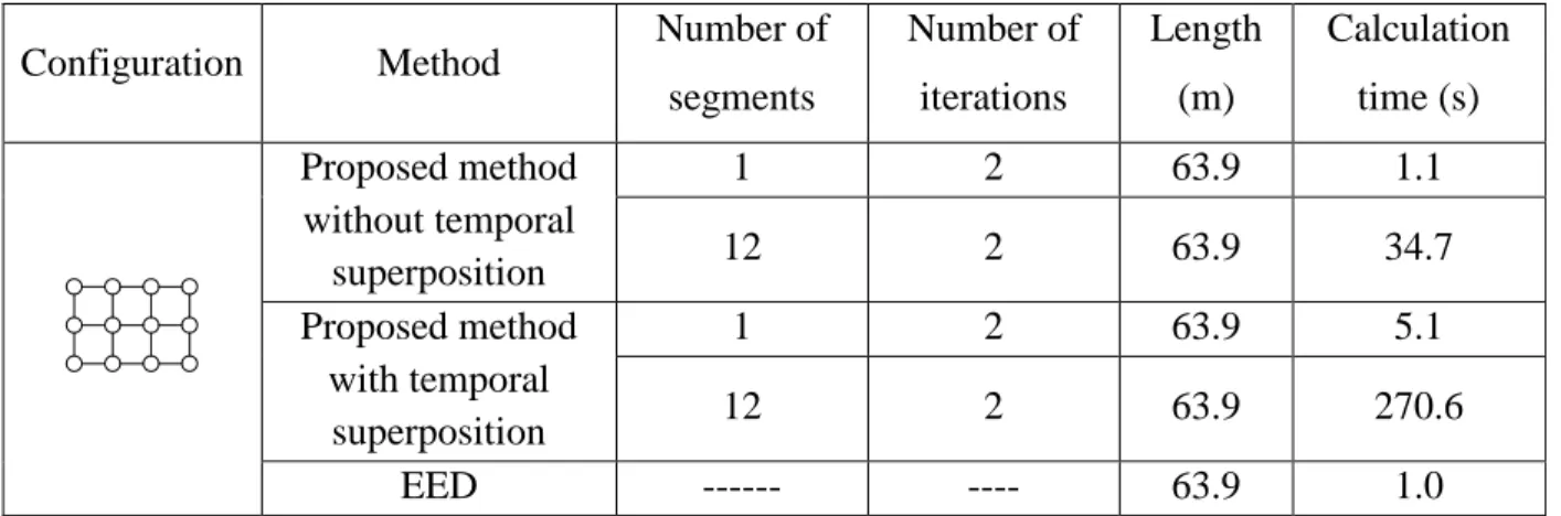
Table 5-4: Comparison between the proposed method and four other sizing tool ... 77

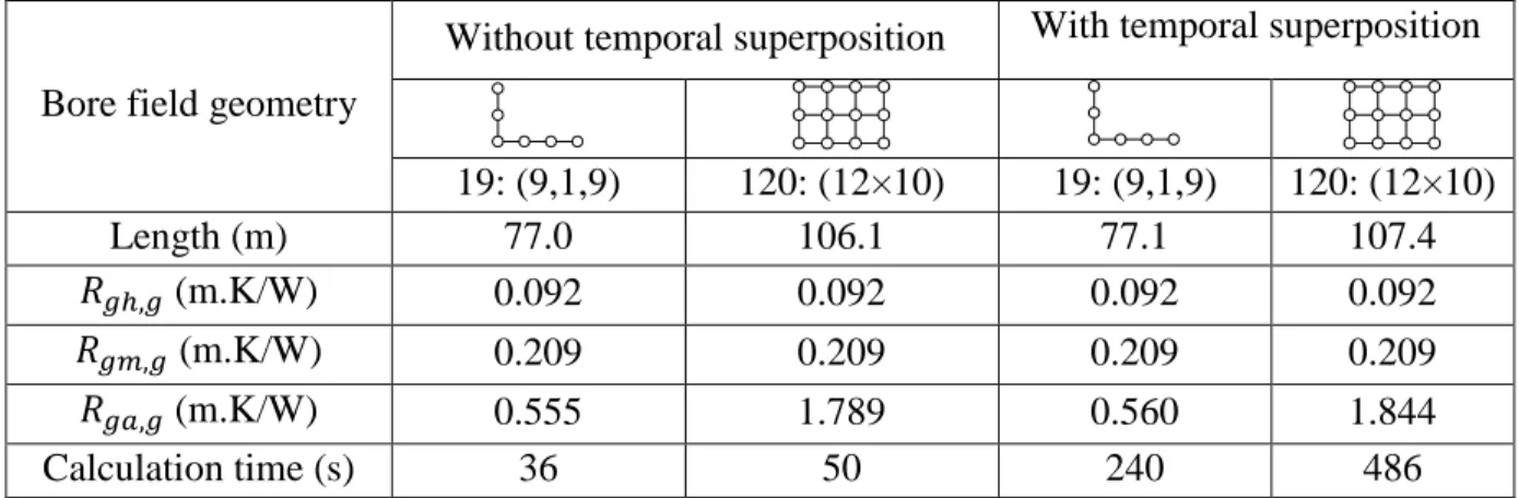
Table 5-5: Comparison of the three ground thermal resistances evaluated with and without temporal superposition ... 78

Table 5-6: Comparison of several methods when there is no annual ground thermal imbalance .. 79

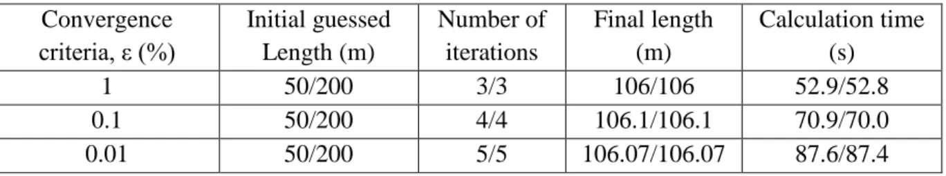
Table 5-7: Analysis of the effects of various convergence criteria and initial guess values on the results ... 80

Table 5-8: Comparison of borehole lengths obtained with and without short time effects ... 84

Table 5-9: The effects of short time effects and peak duration on the boreholes lengths of 12×10 bore field ... 85

Table 6-1: Design parameters used for test case #1 ... 108

Table 6-2: Parameters used in optimization method for test case #1 ... 108

Table 6-3: Borehole lengths determined by GenOpt and the corresponding objective function for test case #1 ... 109

Table 6-4: Performance map for the heat pump used in test case #2 ... 111

Table 6-5: Monthly average and peak building heating and cooling loads used in level 3 for test case #2 ... 113

(15)

Table 6-6: Borehole lengths determined by the proposed methodology and the corresponding

objective function for test case #2 ... 114

Table 6-7: The results of the three sizing levels for test case 2 ... 115

Table 6-8: Values of various parameters used in the optimization of test case #3 ... 117

Table 7-1: Required input parameters for most sizing tools ... 124

Table 7-2: Two different set of inputs to be used with the ASHRAE sizing equation for the Valencia case ... 144

Table 7-3: Input parameters for the four test cases ... 146

Table 7-4: Monthly average and peak ground loads to be used with 𝐿3 methods (all loads are in kW) ... 148

Table 7-5: Synthesis of the data for each Test used in L2 methods (negative values indicate that cooling conditions determine the required length) ... 149

Table 7-6: Sizing tools used in the inter-model comparison ... 152

Table 7-7: Sizing test cases found in the literature ... 173

Table 7-8: Results presented in Figure 7-7 in addition to the mean and individual differences from the mean ... 175

(16)

LIST OF FIGURES

Figure 1-1: Schematic representation of a typical ground source heat pump system ... 1

Figure 2-1: Nomenclature used in the Finite Line Source equation ... 7

Figure 2-2: Nomogram for design of Vertical ground heat exchangers (adapted from Stadler et. al., 1995) ... 21

Figure 2-3: Number of drilled boreholes and their corresponding total drilled meters for a variety of vertical closed loop GSHP systems and a small number of open-loop systems as a function of installed heat pump kilowatt delivery (adapted from a figure presented by Banks (2012)) ... 22

Figure 2-4: General input parameters of most sizing tools ... 31

Figure 2-5: a. A typical hourly load and its b. cooling and c. heating peak heat loads (adapted from content found in GLHEPRO 5.0 (2016)) ... 33

Figure 2-6: a. Temperature responses obtained based on hourly load and three peak load durations for a. cooling peak loads and b. heating peak loads. (Adapted from content found in GLHEPRO 5.0 (2016)) ... 34

Figure 2-7: Temperature responses obtained by “maximum over duration” model (adapted from content found in GLHEPRO 5.0 (2016)) ... 35

Figure 4-1: Three consecutive ground thermal pulses used in Equation 4.1 ... 46

Figure 4-2: Six g-functions curves for a 3 x 2 bore field ... 51

Figure 4-3: Flow diagram of the iterative procedure ... 52

Figure 4-4: Determination of the three g functions related to the three thermal resistances in consecutive iterations ... 53

Figure 5-1: Schematic illustration of a typical GSHP system ... 59

Figure 5-2: Illustration of the five step procedure for the alternative method ... 67

Figure 5-3: Schematic illustration of the thermal interaction of all boreholes segments towards segment #1 ... 68

(17)

Figure 5-4: a. g-Function curves determined with and without the temporal superposition and

their relative difference b. Variation of 𝜃𝑏 ∗ as a function of non-dimensional time ... 72

Figure 5-5: The effect of the number of segments and number of boreholes on ∆, the maximum difference between g-functions evaluated with and without temporal superposition ... 73

Figure 5-6: Ground loads used in the comparison cases ... 74

Figure 5-7: Evolution of the outlet fluid temperature for the last iteration of the DST-GenOpt method ... 80

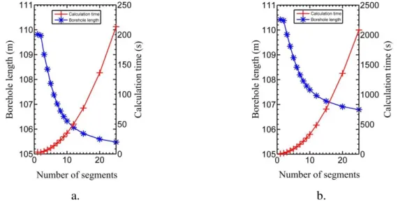
Figure 5-8: Borehole length and corresponding calculation time as a function of the number of segments obtained without (a) with (b) temporal superposition ... 81

Figure 5-9: g-functions obtained with and without short-term effects for a 12×10 bore field ... 83

Figure 5-10: Relative length difference with and without short-term effects ... 85

Figure 6-1: Schematic representation of a typical GSHP system ... 93

Figure 6-2: Three typical ground load pulses and their durations... 95

Figure 6-3: Typical ground loads related to level 2 sizing methods and the variation of 𝑇𝑜𝑢𝑡 related to these loads ... 96

Figure 6-4: Evaluation of three ground heat load pulses and their durations for month j ... 98

Figure 6-5: Six monthly average and peak ground heat load pulses and their durations ... 99

Figure 6-6: Various steps involved in the level 3 sizing methods ... 100

Figure 6-7: The solution procedure of a level 4 sizing method ... 102

Figure 6-8: Geometry used by the DST model for a 37 borehole configuration ... 103

Figure 6-9: a. Schematic illustration of the TRNSYS project, b. Scripted equations used in some of the models. ... 106

Figure 6-10: Ground load used for test case #1 ... 107

Figure 6-11: Plot of the objective function for test case #1 ... 110

Figure 6-12: Evolution of the outlet fluid temperature for the first test case ... 110

(18)

Figure 6-14: Variation of 𝑇𝑜𝑢𝑡, 𝑚𝑎𝑥 over 10 years for each iteration ... 115

Figure 6-15: The objective function of the third test case ... 116

Figure 7-1: Schematic representation of a ground-source heat pump system (left) and a borehole cross-section with one U-tube (right) ... 122

Figure 7-2: Typical steps required to size a bore field for a) 𝐿1 and 𝐿2 methods, b) 𝐿3 and 𝐿4 methods with building loads as input, and c) 𝐿3 and 𝐿4 methods with ground loads as inputs ... 125

Figure 7-3: a) Hourly loads for the synthetic profile; b) Cumulative energy exchange resulting from the hourly loads ... 147

Figure 7-4: Hourly ground loads generated from monthly and peak loads for L4 methods used in Test 2 ... 150

Figure 7-5: Hourly ground load profile for Test 3 ... 151

Figure 7-6: Hourly building loads considered for Test 4 ... 152

Figure 7-7: Inter-model comparison of twelve sizing tools for four test cases ... 154

Figure 7-8: Sensitivity analysis for five parameters compared to the original Test 4 results obtained by each tool ... 158

Figure A-1: Main menu of the Excel spreadsheet designed for sizing vertical boreholes ... 191

Figure A-2: Borehole locations user input worksheet ... 192

Figure A-3: The input parameters required for the ground, borehole, and fluid ... 192

Figure A-4: Input parameters and sizing procedure for the alternative method ... 194

Figure A-5: Input parameters and sizing procedure for the ASHRAE modified method ... 194

Figure A-6: Input parameters for the ASHRAE equation method ... 195

Figure A-7: Input parameters and sizing procedure for the monthly versions of the classic ASHRAE sizing equation and its alternatives ... 197

Figure A-8: Input parameters and sizing procedure for the monthly method with load aggregation ... 197

(19)

Figure A-9: Input parameters and sizing procedure for the monthly methods that use the spectral

method ... 198

Figure A-10: Input parameters required for the evaluation of short and long-term g-functions . 199 Figure A-11: Input parameters required for evaluating temperature penalties ... 199

Figure B-12: Symbols used in the inter-model comparison Excel spreadsheet ... 200

Figure B-13: Example of worksheets used for reporting the input parameters and the results of various sizing tests ... 201

Figure B-14: Building and ground loads given for Test 4 ... 201

Figure B-15: Worksheet used for the sensitivity analysis ... 202

Figure C-16: Typical measured data collected for Valencia case ... 203

Figure C-17: The averaged measured a. fluid flow rate and b. inlet temperature of Valencia case ... 204

Figure C-18: Evolution of the borehole outlet fluid temperature obtained by a. DST, b. Type 245 and c. Type 204 compared to measured values for the Valencia case ... 205

(20)

LIST OF APPENDICES

Appendix A ... 191 Appendix B ... 200 Appendix C ... 203

(21)

CHAPTER 1 INTRODUCTION

Ground source heat pump (GSHP) systems are used increasingly in residential and commercial buildings as they lead to low energy consumption. A typical GSHP system consists of a series of heat pumps connected to a fluid loop and a series of vertical heat exchangers, often called boreholes, embedded in the ground. Compared to air source heat pumps, GSHP systems have higher initial costs. However, on the long term, they have a lower life cycle cost due to their low operating costs.

Given the relatively high costs associated with boreholes (drilling, pipe costs, etc.) it is essential to design them carefully. In particular, the required borehole length should be minimized while providing enough underground surface area to reject or collect heat associated with heat pumps operating in cooling and heating.

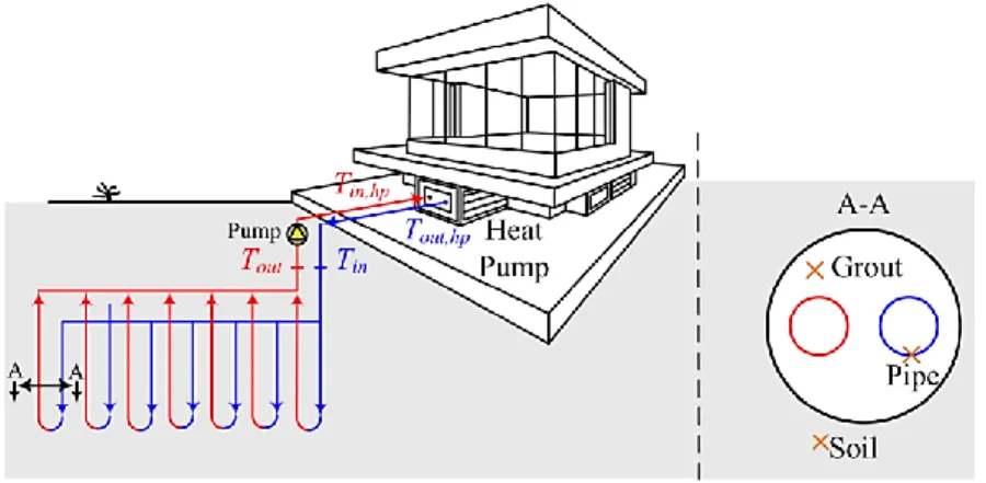
Vertical U-tube boreholes, which are the main focus of this research, typically have a length ranging from 50 to 120 meters and a diameter around 100 to 150 mm. Except for very small buildings. GSHP systems typically use multiple boreholes. Boreholes should be placed at least 6 to 7 meters away from each other to avoid thermal interaction. Boreholes are typically filled with a grout to protect the aquifer and improve heat transfer. The fluid temperature changes as it circulates in the borehole and fluid temperature in the downward and upward legs are different. This may cause a thermal short-circuit between the two legs. Figure 1-1 illustrates schematically a typical GSHP system that consists of seven U-tube boreholes that are connected to a heat pump. Since the U-tubes are connected in parallel to each other, they have the same inlet (𝑇_𝑖𝑛) and outlet (𝑇𝑜𝑢𝑡) temperatures.

(22)

In heating mode, the fluid temperature is lower than the ground temperature and heat is extracted from the ground. Conversely, in cooling mode, heat is rejected into the ground and the circulating fluid temperature is higher than the adjacent ground. The annual amounts of heat injected or rejected are most often unequal. This ground load imbalance can lead to long term ground temperature changes that can reduce the system efficiency or even lead to system failure.

The heat exchanged between the ground and the boreholes depends on many factors such as the ground temperature, the ground thermal properties, the borehole completion method, the bore field configuration and the fluid flow rate. The amount of heat exchanged in the ground depends on the building loads and the heat pump coefficient of performance (COP). Therefore, the required length of vertical ground heat exchangers depends on many factors. The boreholes should be sized so that the return temperature to the heat pumps is within the minimum and maximum operating temperatures.

To properly size vertical ground heat exchangers, many thermal phenomena that occur at different time scales during the operation of the geothermal system should be taken into account. In the short term, i.e. on a scale of several minutes to several hours, the thermal capacities of the fluid, the pipes and the grout are important as they dampen the minimum and maximum fluid temperatures that happen through the operation. In the longer term, i.e. over several years, the thermal interaction between boreholes and the annual ground load imbalances should be taken into account as they may have significant effects.

The main objectives of this study are to review and improve the current methods for sizing vertical ground heat exchangers. The first objective is to improve the ASHRAE sizing equation for vertical ground heat exchangers by removing its dependency on the use of temperature penalties. The proposed methodology uses g-functions to determine the effective ground thermal resistances and is not restricted to rectangular bore field configurations. The g-functions are evaluated “dynamically” as the solution progresses by using the Finite Line Source solution over borehole segments and without using temporal superposition. Indications are given as to the optimum number of segments and recommended convergence criteria. It is also shown how to account for borehole thermal capacity, through the use of short-time step g-functions.

The second objective is to develop an approach that sizes the ground heat exchangers based on multi-year hourly simulations. This is accomplished by combining the DST model in TRNSYS

(23)

with GenOpt, an optimization tool. With this approach, it is possible to minimize one or all three of the following parameters: borehole length, the number of boreholes, and the borehole spacing. The suggested method is able to account for the hourly evolution of the buildings/ground load as well as the changing value of the heat pump COP.

The third objective is to conduct a comparison of the current vertical ground heat exchanger sizing models. The models are first categorized into five levels ranging from rules-of-thumb to sizing methods based on hourly simulations. Then, a series of four test cases are proposed each addressing a particular difficulty. Finally, these test cases are used on twelve different sizing tools in a comprehensive inter-model comparison.

(24)

CHAPTER 2 LITERATURE REVIEW

The relevant literature not discussed in the following chapters is reviewed in this chapter. It covers heat transfer processes used for simulating vertical ground heat exchangers, various sizing models and some of the factors that have significant effects on sizing.

2.1 Heat transfer modeling of vertical ground heat exchangers

Accurate prediction of heat transfer in and around boreholes is essential for sizing vertical ground heat exchangers. Borehole heat transfer can be solved analytically or numerically or in some cases with a combination of both. Analytical models include the Infinite Line Source (ILS) solution (Ingersoll & Plass, 1948), the Infinite Cylindrical Source (ICS) solution (Carslaw & Jaeger, 1946), and the Finite Line Source (FLS) solution (Eskilson, 1987; Zeng et al., 2002), Numerical models can either be based on a Finite Difference method (Lei, 1993; Rottmayer et al., 1997), a Finite Element method (Muraya, 1994; Kohl et al., 2002), or a Finite Volume method (Rees, 2000). Due to computational time requirements and the complexity of their implementation, numerical models are generally not used for ground heat exchanger simulations. Consequently, current sizing models use analytical heat transfer models or pre-calculated numerical solution such as g-functions. It is customary to examine borehole heat transfer inside and outside the borehole separately.

2.1.1 Heat transfer outside the borehole

Heat transfer in the ground outside the boreholes includes heat conduction from the borehole wall to the ground and borehole-to-borehole thermal interaction in the case of bore fields. Heat conduction depends on the thermal conductivity and diffusivity of the ground, the borehole diameter as well as borehole spacing and length. Ground water movement can also be important in some cases.

Most of the GHEs sizing programs that are available today use g-functions that are either evaluated numerically or based on the FLS solution to model heat transfer outside the boreholes. Some programs use the ICS solutions and others use numerical or a combination of analytical and numerical solutions. In the following sections, the general concepts of some of these models are reviewed.

(25)

2.1.1.1 Infinite Line Source model

The ILS is the oldest approach used to calculate heat transfer from ground heat exchangers (Ingersoll & Plass, 1948). It applies Kelvin’s line theory (1882) to obtain the temperature at any point in an infinite medium. The borehole is represented as an infinite long line that has a uniform heat transfer rate per unit length and is inserted in a medium (ground) at a uniform initial temperature. It is a one-dimensional model in the radial direction. Thus, it does not consider heat transfer in the borehole axis direction and thus end effects are neglected. In addition, the inside of the borehole (fluid, pipes, and grout) is not considered. With the ILS, the temperature at any radial point of the ground can be determined by a semi-infinite integral as follows:

𝑇(𝑟, 𝑡) − 𝑇𝑔= 𝑞′ 2𝜋𝑘 ∫ 𝑒−𝛽2 𝛽 ∞ 𝑋= 𝑟 2√𝛼𝑔𝑡 𝑑𝛽 = 𝑞 ′ 2𝜋𝑘𝑔𝐼(𝑋) (2.1)

where 𝑟 is the distance from the borehole’s center line, 𝑇(𝑟, 𝑡) is the ground temperature at 𝑟 for time 𝑡 (when 𝑟 is equal to the borehole radius, the temperature represents the borehole wall temperature at time 𝑡), 𝑇𝑔 is the undisturbed ground temperature, 𝛼𝑔 is thermal diffusivity of the ground, 𝑘𝑔 is the ground thermal conductivity and 𝑞′ is the heat transfer rate per unit length and 𝐼(𝑋) is the solution to the integral. Tabulated values of 𝐼(𝑋) are presented by Ingersoll et al. (1954). Ingersoll et al. (1954) mention that the ILS is accurate when 𝑡>20𝑟_𝑏2 _𝛼

𝑔 ⁄ ..

2.1.1.2 Infinite Cylindrical Source model

Ingersoll et al. (1950) used the solution suggested by Carslaw and Jaeger (1946) to simulate transient heat transfer from an infinite cylinder subjected to a constant heat transfer rate (or constant temperature, (Carslaw and Jaeger, 1959)) in a ground that has uniform initial temperature. Like the ILS, the ICS is a one-dimensional model in the radial direction and it neglects axial variations. The ICS solution is given by:

𝑇 − 𝑇𝑔=

𝑞′

𝑘_𝑔𝐺𝛼𝑔𝑡/𝑟2 (2.2)

where 𝐺 is the 𝐺-factor, 𝛼𝑔𝑡/𝑟2 is the Fourier number, 𝑟 is the distance from the borehole center line and 𝑞′ is the heat transfer rate per unit length. The determination of 𝐺-factors is a fairly

(26)

complex task since it includes integration from zero to inﬁnity of an expression that contains Bessel functions (Eq. 2.3). 𝐺-factors have been calculated and are reported by Ingersoll et al. (1954) and Kavanaugh, (1985). 𝐺_{𝛼𝑔𝑡/𝑟}2 = 1 𝜋2∫ 𝑒−𝑧2(𝛼𝑔𝑡 𝑟_{⁄ )}2 − 1 𝑧2_{( 𝐽} 12(𝑧) + 𝑌12(𝑧)) ∞ 0 [𝐽₀(𝑧 𝑟 𝑟⁄ )𝑌𝑏 1(𝑧) − 𝐽1(𝑧)𝑌0(𝑧 𝑟 𝑟⁄ )]𝑑𝑧𝑏 (2.3)

The ILS and the ICS solutions (Eq. 2.1 and 2.2) are applicable to single boreholes and for a constant heat transfer rate per unit length. For multiple boreholes that have variable heat transfer rates, temporal and spatial superposition are needed to obtain the time evolution of the borehole wall temperature.

2.1.1.3 g-Functions

When the ground heat exchanger operates for a long time, the radial solutions presented by the ILS and the ICS are imprecise. Also, borehole-to-borehole thermal interference becomes important. One way to account for these two phenomenon is to use thermal response factors also known as g-functions based on the pioneering work of Eskilson (1987).

g-Functions are non-dimensional thermal response factors that relate the difference between the borehole wall temperature and the ground temperature to the heat transfer rate per unit length of the boreholes. The g-functions depend on the length and the radius of the boreholes as well as their spacing and are specific to particular bore field configurations. To obtain g-functions, Eskilson (1987) considered the boreholes as finite length cylinders with uniform boundary temperatures in a homogeneous ground at an initial uniform temperature. He used a transient ﬁnite-difference method on radial–axial coordinate system to solve the problem. The heat transfer rate per unit length of the boreholes varies along the borehole length and its variation is dependent on the position of the boreholes in the bore field as well as the operational time. Therefore, temporal and spatial superposition are needed to account for these effects. Equation 2.4 presents the classic definition of g-functions.

𝑇_𝑏− 𝑇_𝑔= 𝑞 ′ 2𝜋𝑘_𝑔𝑔 ( 𝑡 𝑡_𝑠 , 𝑟_𝑏 𝐻, 𝐷 𝐻, 𝑏𝑜𝑟𝑒𝑓𝑖𝑒𝑙𝑑 𝑐𝑜𝑛𝑓𝑖𝑔𝑢𝑟𝑎𝑡𝑖𝑜𝑛) (2.4)

(27)

where 𝑇_𝑏 is the borehole wall temperature, 𝑡_𝑠 is a characteristic time (= 𝐻2⁄9𝛼_𝑔), 𝐻 is the borehole length, and 𝐷 is the buried depth of the top of the borehole. As noted in Equation 2.4, functions depend on four non-dimensional parameters. Finally, according to Eskilson (1987), g-functions are valid for times greater than 5 𝑟_𝑏2 _𝛼

𝑔 ⁄ .

2.1.1.4 Finite Line Source solution

Eskilson (1987) and Zeng et al. (2002) presented the FLS solution. With this approach, the borehole is treated as a source of finite length subjected to a uniform heat transfer rate per unit length and immersed in a ground at an initial uniform temperature. The FLS model is thus a two-dimensional model where axial effects are considered. As shown in Figure 2-1, the FLS solution uses a mirror image above ground to account for the ground surface. When a constant ground surface temperature is assumed, the temperature at point (𝑟, 𝑧) and at time 𝑡 is given by (Eskilson, 1987): 𝑇(𝑟, 𝑧, 𝑡) − 𝑇𝑔= − 𝑞′ 4𝜋𝑘_𝑔∫ [ 𝑒𝑟𝑓𝑐 (√𝑟2+ (𝑧 − ℎ)2 2√𝛼𝑔𝑡 ) √𝑟2_{+ (𝑧 − ℎ)}2 − 𝑒𝑟𝑓𝑐 (√𝑟2+ (𝑧 + ℎ)2 2√𝛼𝑔𝑡 ) √𝑟2_{+ (𝑧 + ℎ)}2 ] 𝑑ℎ 𝐷+𝐻 𝐷 (2.5)

Figure 2-1: Nomenclature used in the Finite Line Source equation

Typically, Equation 2.5 is used to obtain the value of the borehole wall temperature (𝑟 = 𝑟_𝑏) along the length of the borehole. It is often useful to evaluate the mean (often called the mean

(28)

integral) borehole wall temperature over the borehole length. In this case a second integral is required which lead to the following:

𝑇̅(𝑟, 𝑡) − 𝑇𝑔= − 𝑞 ′ 4𝜋𝑘𝑔𝐻∫ ∫ { 𝑒𝑟𝑓𝑐 (√𝑟2+ (𝑧 − ℎ)2 2√𝛼𝑔𝑡 ) √𝑟2_{+ (𝑧 − ℎ)}2 − 𝑒𝑟𝑓𝑐 (√𝑟2+ (𝑧 + ℎ)2 2√𝛼𝑔𝑡 ) √𝑟2_{+ (𝑧 + ℎ)}2 } 𝑑ℎ𝑑𝑧 𝐷+𝐻 𝐷 𝐷+𝐻 𝐷 (2.6)

Diao et al. (2004) used the borehole wall temperature at the mid-length instead of using the mean integral temperature along the borehole to simplify the solution to a single integral. Bandos et al. (2009, 2011) developed an approximation for the integral mean temperature and then used this approximation to evaluate the ground thermal properties based on data captured by a thermal response test. Their model accounts for the effects of the temperature variation on the ground surface as well as the geothermal gradients. Lamarche and Beauchamp (2007b) simplified the solution to Equation 2.6 to one integral for the case that the buried depth is zero (𝐷 = 0). Costes and Peysson (2008) extended the model presented by Lamarche and Beauchamp (2007b) for cases where 𝐷 > 0. Claesson and Javed (2011) present an elegant approach to reduce the number of integrals form two to one for 𝐷 > 0.

It is possible to use the FLS to generate g-functions. Cimmino and Bernier (2013a, 2014) initially used the FLS with a uniform heat transfer rate along the length of each borehole and one segment per borehole to obtain g-functions. The integral mean temperature is used to obtain the borehole wall temperatures. These temperatures are different for each borehole. This boundary condition, referred to as BC-I, leads to g-functions that can be largely overestimated for large bore fields. Improvements can be made to these predictions (Cimmino and Bernier 2013b, 2014) by imposing the same borehole wall temperature to every borehole and varying the heat transfer rate from borehole to borehole. This BC-II boundary condition improves the prediction of the g-functions. However, the borehole wall temperature is still calculated with the mean integral temperature even though the borehole wall temperature varies along the length of the boreholes. In order to adhere to the definition of a g-function as established by Eskilson (1987), the borehole wall temperature has to be uniform along the length of each borehole and constant in the bore field. Cimmino and Bernier (2014) applied this boundary condition, BC-III, by segmenting each borehole and applying the FLS over each of these segments to approach the true boundary condition of Eskilson (1987). With this approach, Cimmino and Bernier (2014) have shown that

(29)

it is possible to reproduce the original numerically-generated g-functions with relatively high accuracy. Their proposed methodology can account for boreholes that have different lengths and various buried depths. Recently, Lamarche (2017) modified the model presented by Cimmino and Bernier (2014) by introducing a linear heat transfer rate per unit length instead of a piecewise constant distribution profile along the borehole. The new model evaluates the results with the same precision as the model of Cimmino and Bernier (2014) with fewer segments.

2.1.2 Heat transfer inside the borehole

Various heat transfer processes occur inside the borehole including convective heat transfer between the fluid and the U-pipes inner wall, heat conduction in the pipe thickness and in the grout from the pipes to the borehole wall.

Generally, it is advantageous to have the lowest borehole thermal resistance to lower borehole length. When inlet conditions do not change significantly with time, it is possible to assume steady-state heat transfer in the borehole. For these cases, a steady-state borehole thermal resistance, 𝑅𝑏, is typically used. For rapidly changing inlet conditions (temperature and/or flow rate) it is necessary to model transient heat transfer in the borehole as the thermal capacitance of the grout/fluid have a significant impact in damping the fluid temperature variations. Ignoring these short-term thermal effects can lead to an error in determination of the energy consumption of the system (Salim-Shirazi and Bernier, 2013) and an overestimation of the required borehole length.

2.1.2.1 Steady-state

Javed and Spitler (2017) have provided an excellent review on methods to evaluate 𝑅𝑏. Values of 𝑅_𝑏 are local values. When heat transfer from the downward and upward legs is important (e.g. for low flow rates and/or long boreholes), the thermal short-circuit has to be considered. One way to achieve this is to calculate an effective borehole thermal resistance, 𝑅_𝑏∗_{, Javed and Spitler (2016).} Steady-state borehole thermal resistances can be obtained experimentally from a thermal response tests (Shonder and Beck, 1999, Austin et al., 2000, Gehlin and Hellström, 2003) or analytically by using the borehole and ground thermal properties. Lamarche et al. (2007c, 2010) and Javed et al. (2009, 2010) have presented good reviews of the analytical methods that can be used for the evaluation of the boreholes thermal resistances.

(30)

Heat transfer inside the borehole has been treated as a quasi-three-dimensional problem (Dobson et al., 1995; Zeng et al., 2002). If one neglects the variation of the fluid temperature along the borehole length, the heat transfer inside the borehole can be simplified to a two-dimensional problem (Yavuzturk et al., 1999, Rees, 2000). It is also possible to reduce the problem to one-dimensional radial conduction by using an equivalent concentric cylinder (Deerman and Kavanaugh, 1991).

A conventional method for the evaluation of borehole thermal resistances is to use a circuit of thermal resistances connecting the fluid in each pipe to the borehole wall. Hellström (1991) used such an approach. He obtained the internal thermal resistances using two models: the line source model and its more general derivative, the multipole method. The multipole method was first suggested by Claesson and Bennet (1987) and Bennet et al. (1987) and recently improved by Claesson and Hellström (2011).

Hellström (1991) explains that the effect of varying fluid temperature along the U-tubes as well as the heat exchange between the legs can be evaluated by an effective fluid to ground thermal resistance 𝑅_𝑏∗_:

𝑇̅ (𝑡) − 𝑇_𝑓 ̅̅̅(𝑡) = 𝑞_𝑏 ̅ 𝑅′

𝑏∗ (2.7)

where 𝑇̅ is the average of the inlet and outlet temperatures, 𝑇_𝑓 ̅̅̅ is the average borehole wall _𝑏 temperature and 𝑞̅ is the heat transfer rate per unit length of the boreholes. In the case of ′ Equation 2.7, the effective borehole thermal resistance, 𝑅_𝑏∗_{, applies to the entire borehole and not} locally like 𝑅𝑏.

Hellström (1991) then evaluates the effective thermal resistance for the two cases of uniform temperature and uniform heat flux along the borehole. For the uniform temperature case, 𝑅_𝑏∗ is determined as follows: 𝑅_𝑏∗ _{= 𝑅} 𝑏𝜂 𝑐𝑜𝑡ℎ(𝜂) (2.8) 𝜂 = 𝐻 𝐶𝑓𝑉𝑓2𝑅𝑏√1 + 4 𝑅_𝑏 𝑅₁₂∆ (2.9)

(31)

where 𝐻 is the borehole length, 𝐶_𝑓 is the fluid specific heat, 𝑉_𝑓 is mass flow rate, 𝑅_𝑏 is the local borehole thermal resistance without the short circuit effects and 𝑅₁₂∆ is the thermal resistance of the ∆ circuit between the two pipes. The factor 𝜂 𝑐𝑜𝑡ℎ(𝜂) gives the correction for the fluid temperature variation along the U-tubes and it can be estimated by 1 + 𝜂2⁄ when 𝜂 ≤ 1. A 3 series expansion for small values of 𝜂 gives:

𝑅_𝑏∗ _{≈ 𝑅} 𝑏+ [ 1 3𝑅₁₂∆ ( 𝐻 𝐶_𝑓𝑉_𝑓) 2 + 1 12𝑅_𝑏( 𝐻 𝐶_𝑓𝑉_𝑓) 2 ] 𝜂 ≤ 1 (2.10)

For the case of uniform heat flux along the borehole, 𝑅_𝑏∗_{is evaluated as:}

𝑅_𝑏∗ _{≈ 𝑅} 𝑏+ [ 1 3𝑅_𝑎( 𝐻 𝐶_𝑓𝑉_𝑓) 2 ] (2.11)

where 𝑅_𝑎 is the product of a parallel-coupling of two parts: the thermal resistance between the pipes and the two thermal resistances between each pipe and the borehole wall that are coupled in series. In Equations 2.10 and 2.11, the terms that are in brackets account for the fluid temperature variation along the length as well as the heat exchange between the legs.

Zeng et al. (2003) and Diao et al. (2004) used a quasi-three-dimensional model to evaluate the heat transfer inside the boreholes that have uniform wall temperatures. The model accounts for the variations of the fluid temperature and pipe wall temperature through the axial direction and the impact of the short-circuiting among U-tube legs for different fluid circuit arrangements in double U-tubes boreholes. The results are obtained by Laplace transformation and it is showed that the double U-tubes arranged in parallel have better performance than the ones in series (Zeng et al. 2003).

Simplifying the two pipes into a single equivalent diameter pipe helps to simplify the heat transfer inside the borehole in the radial direction. Various approaches can be used to evaluate the equivalent diameter pipe (Bose et al., 1985, Gu and O’Neal, 1998, Kavanaugh, and Rafferty, 1997, Sutton et al., 2002).

Sutton et al. (2002) used the infinite cylindrical heat source solution to simulate heat transfer inside the boreholes. In their model, the convection thermal resistance of the fluid and the conductive thermal resistance of the pipes are neglected and the calculations are done just based

(32)

on the grout thermal properties. The U-tubes are simplified into an equivalent diameter pipe. The radius of this pipe is determined based on the borehole thermal resistance, which is evaluated with the solution proposed by Paul (1996).

2.1.2.1 Transient state

Beier and Smith (2003) developed a model that takes the thermal capacity of the fluid and the grout into account and neglects the conduction and the convection thermal resistances of the pipes and the contact resistances between the pipes and the grout. Based on these assumptions, the fluid and pipe temperatures are equal. The two pipes in the borehole are simplified to a single pipe with an equivalent diameter. The resulting one-dimensional model that simulates the temperature change in the grout and separately in the ground around the borehole is solved by Laplace transforms.

Young (2004) used the Buried Electrical Cable (BEC) model introduced by Carslaw and Jaeger (1959) for the evaluation of short-term effects in boreholes. In this model, called the borehole fluid thermal mass model (BFTM model), the boreholes are simulated as infinite cylinders inserted in a ground with uniform properties. The heat transfer inside each borehole is simulated by a core (with an equivalent diameter for the U-tubes) that is surrounded by insulation and a sheath. The core and the sheath are assumed to play the role of the fluid and the grout and have infinite conductivities and finite thermal capacitance. The insulation is assumed to play the role of the borehole thermal resistance evaluated based on the multipole method (Bennet et al., 1987). It has a finite thermal conductivity and no thermal capacitance. They used a fluid factor to account for fluid outside the borehole. In addition, they used a grout allocation factor (GAF) to adjust the grout thermal mass between the fluid and the grout and a logarithmic extrapolation procedure to improve the accuracy of the model. The grout allocation factor actually transfers a fraction of grout thermal capacity to the fluid and it depends on factors such as borehole diameter and shank spacing. Thus, it varies from case to case and is not easy to evaluate.

Lamarche and Beauchamp (2007c) solved a problem similar to the one considered by Beier and Smith (2003) in the time domain by using Laplace transforms. The model solves the exact solution for concentric cylinder heat exchangers and gives a good approximation for the U-tube heat exchangers. Heat transfer inside and outside the borehole are modeled with two different governing equations and the thermal properties of both the grout and the ground are accounted

(33)

for. The problem is solved for two conditions: i) imposed heat transfer rate per unit length at the pipes and ii) given mean fluid temperature and convention heat transfer through the pipes. For both cases, it is showed that the obtained solutions agree with the classic solutions when the grout and the ground materials are the same and these simplified cases are used for validation of the proposed method. In addition, the model is compared to four other methods including the buried cable method suggested by Young (2004), the compound model solution suggested by Sutton et al. (2002), a numerical solution based on COMSOL, and a model that uses a constant steady-state borehole thermal resistance. The suggested model matches perfectly the results from COMSOL. The buried cable model is shown to be more accurate than the classical methods but it deviates at very short time steps. The method suggested by Sutton et al. (2002) is accurate for short time steps but it has a deviation for longer time periods.

Bandyopadhyay et al. (2008a) used the classic Blackwell solution to solve heat transfer inside the borehole. In this model, the fluid is assumed to be virtual solid, with a diameter equivalent to the two pipes of the U-shaped loop, at a uniform temperature that injects constant heat at the borehole center. The model is only suitable for cases where the grout and ground have the same thermal properties. The same authors extend this approach with a semi-analytical model in which the properties of the grout and ground are different (Bandyopadhyay et al., 2008b). In this model, the solution is obtained in the Laplace domain and inverted with a numerical Gaver-Stehfest algorithm (Stehfest, 1970) in the time domain. The results of the model compare favorably well with the ones determined with a finite element method.

Yavuzturk et al. (2009) developed a finite element model to simulate transient heat transfer inside boreholes. The proposed model, developed as a TRNSYS component, uses the short time step temperature response factors (g-functions) coupled with a finite element model to simulate the inside of the borehole. The two-pipe geometry is converted into an equivalent diameter pipe. The borehole wall is actually the boundary that couples the finite element model to the ground thermal response factors and so the temperature and heat flux of this boundary should be similar in both models. The results issued from this model compares favorably well with the composite cylinder with fluid thermal mass solution introduced by Beier and Smith (2003). By comparing the model to the results obtained by Yavuzturk and Spitler (1999), it is observed that when the borehole thermal resistance is assumed to vary in time, the temperature profile takes 15 to 20 hours to follow the temperature profile modeled with a steady-state borehole thermal resistance.

(34)

Javed et al. (2010) and Javed and Claesson (2011) proposed an analytical model to simulate the short term temperature response of vertical ground heat exchangers. In the applied model, the U-tubes are replaced by a pipe with an equivalent diameter and the thermal resistance and thermal capacities of all ground heat exchanger elements are taken into account. Borehole heat transfer is solved in the Laplace domain with the use of a circuit of thermal resistances and by using inverse transforms to revert it back to the time domain. The authors compared their results to the BFTM of Young (2004), the solution suggested by Lamarche and Beauchamp (2007) and the virtual solid solution introduced by Bandyopadhyay et al. (2008a). These models are compared for three different borehole completion method: i) filled with ground water, ii) backfilled with thermally enhanced grout and iii) backfilled with borehole cuttings. The authors explained that the model suggested by Young assumes that the grout and the fluid have lumped thermal capacities and temperatures which is not correct in reality. In addition, the grout allocation factor and the logarithmic extrapolation that are suggested in this model are ambiguous to calculate and this model is the most inaccurate one for all three filling conditions. The model suggested by Lamarche and Beauchamp (2007) does not account for the fluid thermal capacity and this causes its results to be inaccurate for short times; however its results merge to the results of the suggested method on the long term. The model introduced by Bandyopadhyay et al. (2008a) is also shown to be inaccurate since the boreholes are assumed to be backfilled with borehole cuttings which does not happen often in reality.

So-called thermal resistance capacitance (TRC) models can also simulate the short-term behavior of boreholes. Bauer et al. (2010, 2011) made the initial contribution in this area followed by Zarella et al. (2011) and Pasquier and Marcotte (2012, 2014). In most cases, TRC models can also account for axial variations.

Li and Lai (2012) used the infinite linear source solution in a composite medium to obtain short-term response factors. The line sources are positioned according to the position of the pipes in the borehole and are superimposed spatially. The thermal responses are evaluated at the pipe wall and so the thermal resistance of the borehole is evaluated implicitly. The solution is mentioned to be valid until the axial effects appear. Later, Yang and Li (2014) used the finite volume method as well as some measured experimental data to check the validity of the composite medium line source model. The results showed that except for very short time periods, the results of both numerical and analytical models match each other but they are both higher than the experimental

(35)

data. For short periods (3 to 4 min), it is observed that the composite line source does not have the sufficient accuracy and so the authors have suggested to use this model for simulations of more than 3 minutes.

Salim-Shirazi and Bernier (2013) used the finite volume model coupled to the cylindrical source solution to simulate the boreholes outlet fluid temperature for varying inlet temperature and flow rate. In the applied model, the axial and azimuthal temperature variations are neglected and only the radial variations are accounted. The fluid and the grout thermal capacities are also accounted and an equivalent geometry consisting of a single pipe and a cylinder core filled with the grout is used. The developed model is compared to some analytical and numerical models as well as the experimental data presented by Spitler et al. (2009). Simulations of a building equipped with an on/off heat pump showed that neglecting the thermal capacity of the grout and the fluid leads to an overestimation of the heat pump energy consumption.

As described earlier, the original g-functions are used to evaluate heat transfer from the borehole wall to the ground. Therefore, they were not originally intended to predict the thermal behavior inside boreholes for short-time steps, i.e. for times less than 5𝑟_𝑏2⁄ (it is typically 9 hours when 𝛼𝑔 𝑟_𝑏 = 0.075 m and 𝛼_𝑔=0.075 m2/day). However, for sizing or simulating the operation of vertical ground heat exchangers correctly, it is important to predict the short-term behavior of the borehole.

Yavuzturk and Spitler (1999) and Yavuzturk et al. (1999) extended the long-term g-function and presented so-called short-time g-functions. To evaluate the g-functions for short time steps, they used a two-dimensional (in polar coordinates), fully implicit ﬁnite volume formulation that uses “pie-sector” representation of the U-tubes. The thermal capacitance of the grout, the pipes and the fluid are included in the calculations. In order to follow the g-function definition introduced by Eskilson, the authors subtracted the contribution of the steady-state borehole thermal resistance of the borehole from the thermal response. This leads to negative g-functions for very short-time periods. In effect, when using short-time g-functions, the borehole wall temperature is obtained using: 𝑇_𝑏− 𝑇_𝑔 = 𝑞′_(𝑅 𝑏+ 𝑔_𝑠ℎ(_𝑡𝑡 𝑠 , 𝑟𝑏 𝐻 ) 2𝜋𝑘 ) (2.12)

(36)

where 𝑅𝑏 is the borehole thermal resistance and 𝑔𝑠ℎ is the short-time g-fucntion. The g-function takes the value of −2𝜋𝑘𝑅𝑏 when 𝑇𝑏= 𝑇𝑔 for 𝑡 = 0. As time progresses, the g-function values gradually increase and become positive after a certain time. The generated short time-step g-functions line up very well with Eskilson’s long time-step g-g-functions indicating the validity of the approach proposed by (Yavuzturk and Spitler, 1999). Transient effects in the borehole can be considered negligible when the short-term and long-term g-function curve merges. This approach has also been modified to handle variations of borehole thermal resistance which can occur with fluid flow rate variations. The model has been validated successfully against the operational data of an elementary school (Yavuzturk and Spitler, 2001).

Xu and Spitler (2006) used a one-dimensional numerical model to calculate the short-term g-functions. The model uses an equivalent concentric cylinder geometry with five elements (a fluid layer, an artificial convective resistance layer, a tube layer, a grout layer and the surrounding ground) to represent the borehole. It is also possible to account for the thermal effects of the fluid outside the boreholes by using a fluid factor. The one-dimensional thermal resistances are calibrated so that they always match the total two-dimensional resistance that can be determined by the multipole method (Bennet et al., 1987). By controlling these parameters, the one-dimensional model compares favourably well with the two-one-dimensional boundary-fitted coordinates GEMS2D model (Rees, 2000) at a significantly lower computational cost (Xu, 2007).

2.2 Vertical ground heat exchanger sizing models

In this work, the sizing models are categorized into five levels based on the type of ground/building loads that they use. These levels are as follows:

Level 0- Rules of thumb, graphical charts and correlated equations Level 1- Two load pulse methods

Level 2- Three load pulse methods

Level 3- Monthly average and peak load pulses Level 4- Hourly loads

(37)

These levels and the most important underlying methods are reviewed in chapter seven. For completeness, the following section describes the models that are not discussed in chapter seven.

2.2.1 Level 0

2.2.1.1 Rules of thumb

The simplest way of sizing ground heat exchangers is to use rules of thumb. Rules of thumb relate the length of the ground heat exchangers to the peak heating or cooling loads of the building or to the installed capacity of the heat pump.

Rules of thumb are often used in small residential buildings where the experience of the installer dictates the required length based on the installed capacity of the heat pump. However, for large bore fields with large annual ground thermal imbalances, rules of thumb may result in large errors. In addition, rules of thumb do not account for the effects of design temperatures (maximum and minimum entering heat pump fluid temperatures) or many other design factors such as the borehole thermal resistance. Following is a review of rules of thumb used in various countries.

Rules of thumb up to 1983

Ball et al. (1983) reviewed borehole sizing models developed up to 1983 and categorized sizing models into three groups: rules of thumb, steady state models and transient models.

The authors state that rules of thumb have served well when the ground and weather conditions were fairly similar from one project to the next. However, they do not give good results for short boreholes, small borehole spacing, and high extraction rates. In addition, they mention that rules of thumb should not be extrapolated to other ground or weather conditions. The authors have presented various rules of thumb in a table similar to Table 2-1. Unfortunately, these rules are unclear and difficult to interpret.

The rules of thumb presented in Table 2-1 can be compared to the results of a study presented by Caneta (1998). In this study, the operational details of nine commercial/institutional buildings equipped with ground source heat pump systems located in the United States and Canada are analyzed. The results are summarized as follows: average building floor area 45900 ft2 (range from 8000 ft2 to 181069 ft2), average heat pump capacity of 111 tons (range from 24 to 410 tons),

(38)

average flow rate of 2.46 gpm/ton (range from 0.4 to 3.2 gpm/ton), average vertical borehole length of 131 ft/ton (range from 92-176 ft/ton). By multiplying the last value by two, the average piping length is determined as 262 ft/ton (range of 184-352 ft/ton) which is within the values reported for copper/steel piping in Table 2-1.

Table 2-1: Rules of thumb reported by Ball et al. (1983)

Parameter Reference

 Piping length, m/kW (ft./ton) of heating or cooling

19 to 37 (215 to 430) with copper/ steel piping (Ambrose, 1966)

28 to 37 (320 to 430) with plastic piping (Bose, 1981)

9 (108) wetted vertical piping (Bose, 1981)

36 (413) European experience (20 W/m) (21 Btu/(h.ft.)) average heat extraction rate at COP of 3.0

 Burial depth m (ft.) 1.3 (4.3) with cooling

0.5 to 0.8 (1.6 to2.6) Without cooling (Oskarsson, 1981)

 Spacing m (ft.)

1.3 to 1.6 (4.3 to 5.2) (Oskarsson, 1981)

 Outside diameter of piping

Ground heat flow to piping is independent of diameter (Vestal and Fluker, 1956)

Size inside diameter to minimize pumping power  Circulation rate

0.04 to 0.07 L/(s.kW) (2 to 4 gpm/ton) (Bose, 1982)

Reynolds number high enough to be above laminar flow but low enough to minimize pumping power i.e. 5000 to 10000

Ball et al. (1983) also explained that up to the 1983 no general design guidelines or publicly available design methodology were available in the United States or in Europe. Furthermore, the available models are both too detailed and expensive to use or too simple and not much more accurate than rules of thumb.

(39)

Germany

In Germany, the lengths of borehole heat exchangers are often less than 100 m deep as longer boreholes need special permissions according to the German mining law. The temperature difference between the fluid in the boreholes and the undisturbed ground must not exceed ±10 °C under average load and ±15 °C under peak load conditions.

The German Guideline (Richtlinien, 2001) makes a distinction between small systems that have heating power less than 30 kW and larger ones. Small systems can be designed with a table of values and a nomogram, whereas the bigger systems should be designed by computer simulations. A part of this table is presented in Table 2-2. As can be seen, the specific heat extraction rates can be used for design of vertical ground heat exchangers in different geological conditions. As an example, based on Table 2-2, when a house has 2400 annual full load heating hours and the ground thermal conductivity is 2.0 W/m-K, the borehole heat extraction rate is about 50 W/m. If the heating power is assumed equal to 12 kW and the seasonal performance factor is 3.13, then the total required length would be 163.2 m (=12 kW/50 W/m ×(3.13-1)/3.13). As this length is more than 100 m, two boreholes of 81.6 m can be used.

Table 2-2 is restricted to the following conditions: Borehole lengths: 40 – 100 m, borehole spacing: 5 m for 40 –50 m and 6 m for 50 –100 m boreholes, double U pipes DN20, DN25 or DN32 or coaxial borehole with more than 60 mm in diameter. Only heat extraction (which may include production of hot water) is considered. The extraction power of boreholes that have thermal interferences has to be reduced by 10 –20 %. In cases that have less than 1000 hours of operation per year the length of the boreholes can be reduced by around 10 %. In summary, under the German guidelines, the required total length of the borehole should be determined based on the amount of heat that is to be withdrawn per meter. For grounds that have low thermal conductivities, such as dry sand, heat extraction rates are around 20 to 25 W/m while high thermal conductivity grounds, such as granite, heat extraction rates of 70 to 84 W/m are reported.

(40)

Table 2-2: Some typical rules of thumb based on German guidelines

Underground Specific heat extraction

General guideline values 1800 h/y 2400 h/y

Poor underground (dry sediment), 𝑘𝑔<1.5 W/m.K 25 W/m 20 W/m

Normal rocky underground and water saturated sediment, 1.5<𝑘𝑔 <3 W/m.K 60 W/m 50 W/m

Consolidated rock with high thermal conductivity, 𝑘𝑔 >3 W/m.K 84 W/m 70 W/m

Individual rocks

Gravel, Sand, dry <25W/m <20W/m

Gravel, Sand, water saturated 65-80 W/m 55-65 W/m

For strong groundwater flow in gravel and sand, for individual systems 80-100 W/m 80-100 W/m

Switzerland

The Swiss Bundesamt Für Energie wirtschaft (Stadler et al., 1995) has developed a nomogram, similar to the one reproduced in Figure 2-2, for sizing of small systems located in Switzerland. The nomogram is developed based on the results of computer simulations and was not validated by field monitoring. As can be seen, by using this nomogram, the length of single and double U-tube boreholes can be determined based on the annual heating energy, the heating power and the climatic conditions of the building which is defined based on the altitude of the building’s location. A nomogram factor, 𝑎, defined in Equation 2.13 is required for using the nomogram.

𝑎 = 𝑄𝐻𝑎

𝑄_𝐻𝑎⁄𝛽_𝑎− 𝑄_𝑝𝑎 (2.13)

where 𝑄_𝐻𝑎 is the annual heating energy in kWh/year, 𝑄_𝑝𝑎 is the annual energy demand of peripheral components (circulation pump) in kWh/year, and 𝛽_𝑎 is seasonal performance factor. The use of the nomogram is presented here with the example introduced in previous section. The house requires 2400 full load heating hours per year and the required power is 12 kW, then the annual heating energy, 𝑄_𝐻𝑎, is equal to 28.8 MWh/year (12 kW×2400 h) which is out of the specified range of heating energy (4–16 MWh/year) in the nomogram. Therefore, it is assumed that the total energy is provided by two boreholes with no thermal interactions (each provide 14.4 MWh/year with a heating power of 6 kW). Assuming that the power of peripheral components is

(41)

equal to 0.4 kW, the annual required energy (𝑄_𝑝𝑎) is 0.96 MWh/year (=0.4 kW×2400h). As a result, the nomogram factor is 4.0 (=14.4/(14.4/3.13-0.96)). If the house is assumed to be located at an altitude of 300 m, the resulting length of each borehole is around 75 m. This length can be compared to the length of 81.6 m determined earlier with Table 2.2.

Figure 2-2: Nomogram for design of Vertical ground heat exchangers (adapted from Stadler et. al., 1995)

England

Banks (2012) has presented a figure, similar to the one reproduced in Figure 2-3, based on data gathered from some documented case studies. The figure reports the number of boreholes (left axis) and the total drilled meters (right axis) as a function of the heat pump delivery (in kW). It should be noted that all axes have logarithmic scales.

As mentioned by Banks (2012), most of these cases are either constructed or designed in the United Kingdom. The majority of data presented in Figure 2-3 are for heating dominated cases. However, some of the larger systems (more than 60 kW) are cooling dominated or provide both cooling and heating. As shown on this figure, the open loop systems extract more heat per borehole compared to closed loop systems. The installed capacity per borehole ranges from 2 to 17 kW. The smallest installed capacities are related to the shallowest (40 m) and the highest to

0 4 8 12 16 20 0 2 4 6 8 10 W/m-K Kg =1.2, 2.0, 3.6 H ea ti n g e n er g y ( M W h /y ) Heating Power (kW) 2000 1600 1200 800 400 0 A lt it u d e (m ) N o m o g ra m f ac to r (a ) 3 5 4 B o re h o le s le n g th ( m ) 0 40 80 120 160 200 Number of boreholes 1 2 60 120 80 100