An Empirical Analysis of U.S. Aggregate Portfolio Allocations

Texte intégral

(1)2005s-07. An Empirical Analysis of U.S. Aggregate Portfolio Allocations Michel Normandin, Pascal St-Amour. Série Scientifique Scientific Series. Montréal Mars 2005. © 2005 Michel Normandin, Pascal St-Amour. Tous droits réservés. All rights reserved. Reproduction partielle permise avec citation du document source, incluant la notice ©. Short sections may be quoted without explicit permission, if full credit, including © notice, is given to the source..

(2) CIRANO Le CIRANO est un organisme sans but lucratif constitué en vertu de la Loi des compagnies du Québec. Le financement de son infrastructure et de ses activités de recherche provient des cotisations de ses organisations-membres, d’une subvention d’infrastructure du Ministère du Développement économique et régional et de la Recherche, de même que des subventions et mandats obtenus par ses équipes de recherche. CIRANO is a private non-profit organization incorporated under the Québec Companies Act. Its infrastructure and research activities are funded through fees paid by member organizations, an infrastructure grant from the Ministère du Développement économique et régional et de la Recherche, and grants and research mandates obtained by its research teams. Les organisations-partenaires / The Partner Organizations PARTENAIRE MAJEUR . Ministère du Développement économique et régional et de la Recherche [MDERR] PARTENAIRES . Alcan inc. . Axa Canada . Banque du Canada . Banque Laurentienne du Canada . Banque Nationale du Canada . Banque Royale du Canada . Bell Canada . BMO Groupe Financier . Bombardier . Bourse de Montréal . Caisse de dépôt et placement du Québec . Développement des ressources humaines Canada [DRHC] . Fédération des caisses Desjardins du Québec . GazMétro . Groupe financier Norshield . Hydro-Québec . Industrie Canada . Ministère des Finances du Québec . Pratt & Whitney Canada Inc. . Raymond Chabot Grant Thornton . Ville de Montréal . École Polytechnique de Montréal . HEC Montréal . Université Concordia . Université de Montréal . Université du Québec . Université du Québec à Montréal . Université Laval . Université McGill . Université de Sherbrooke ASSOCIE A : . Institut de Finance Mathématique de Montréal (IFM2) . Laboratoires universitaires Bell Canada . Réseau de calcul et de modélisation mathématique [RCM2] . Réseau de centres d’excellence MITACS (Les mathématiques des technologies de l’information et des systèmes complexes) Les cahiers de la série scientifique (CS) visent à rendre accessibles des résultats de recherche effectuée au CIRANO afin de susciter échanges et commentaires. Ces cahiers sont écrits dans le style des publications scientifiques. Les idées et les opinions émises sont sous l’unique responsabilité des auteurs et ne représentent pas nécessairement les positions du CIRANO ou de ses partenaires. This paper presents research carried out at CIRANO and aims at encouraging discussion and comment. The observations and viewpoints expressed are the sole responsibility of the authors. They do not necessarily represent positions of CIRANO or its partners.. ISSN 1198-8177.

(3) An Empirical Analysis of U.S. Aggregate Portfolio * Allocations Michel Normandin†, Pascal St-Amour ‡. Résumé / Abstract Ce papier analyse la forte variation chronologique dans les portefeuilles agrégés américains. À cet effet, nous utilisons des descriptions flexibles des préférences et des opportunités d'investissement afin de dériver les allocations tactiques, myopes et stratégiques. Ces règles sont ensuite comparées aux données dans le cadre d'une analyse statistique formelle. Nos principaux résultats révèlent que i) les règles purement myopes ou tactiques sont rejetées, ii) les portefeuilles stratégiques sont supportés et iii) les facteurs Fama-French sont ceux qui reproduisent le mieux les allocations empiriques. Mots clés : modèles factoriels des rendements, myopes et stratégiques, portefeuilles tactiques, utilité non espérée. This paper analyzes the important time variation in U.S. aggregate portfolio allocations. To do so, we first use flexible descriptions of preferences and investment opportunities to derive optimal decision rules that nest tactical, myopic, and strategic portfolio allocations. We then compare these rules to the data through formal statistical analysis. Our main results reveal that i) purely tactical and myopic investment behaviors are unambiguously rejected, ii) strategic portfolio allocations are strongly supported, and iii) the Fama-French factors best explain empirical portfolio shares. Keywords: factorial models of returns, myopic and strategic, non-expected utility, tactical portfolio allocations. *. Normandin acknowledges financial support from Fonds Québécois de la Recherche sur la Société et la Culture and Social Sciences and Humanities Research Council. St-Amour acknowledges financial support from the Swiss National Science Foundation. This research is carried out within and also funded by the National Center of Competence in 'Research Financial Valuation and Risk Management'. The National Centers of Competence in Research are managed by the Swiss National Science Foundation on behalf of the Federal authorities. The authors are grateful to Raman Uppal for helpful suggestions. The usual disclaimer applies. † Department of Economics and CIRPÉE, HEC Montréal, 3000 Chemin de la Côte-Ste-Catherine, Montréal, Québec, Canada, H3C 3P8. Tel: (514) 340-6841. Fax: (514) 340-6469. E-mail: Michel.Normandin@hec.ca. ‡ Corresponding author: École des HEC, University of Lausanne, FAME, CIRANO and CIRPÉE. Correspondence: University of Lausanne, École des HEC, CH-1015 Lausanne, Switzerland. E-mail: Pascal.StAmour@unil.ch, Tel.: (41) 21.692.34.77. Fax.: (41) 21.692.33.65..

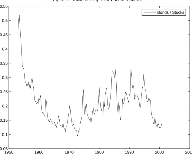
(4) Introduction One striking features of U.S. aggregate portfolio allocations is that holdings of cash, bonds, and stocks relative to wealth exhibit pronounced fluctuations through time. Specifically, from the mid 70’s to the late 80’s the empirical share of cash drastically increased, holdings of stocks substantially decreased, while the demand of bonds mildly declined (see Figure 1). This seems at odds with a prediction associated with tactical portfolio allocations, namely that portfolio rules are time-invariant. These decision rules are optimal regardless of the investors’ risk aversion, as long as the investment opportunity set is constant. Under such an environment, investors do not perform dynamic hedging because shocks to state variables have no effect on future asset returns. Thus, investors act as if their planning horizon is only one period. This reflects the behavior of short-term investors.. [ Insert Figure 1 here ] Another important characteristic of U.S. aggregate portfolio allocations is that the empirical shares display different dynamic properties. In particular, the ratio of the empirical share of bonds to that of stocks falls dramatically between the early 50’s and 70’s, and displays strong upward swings afterwards (see Figure 2). This seems inconsistent with a prediction derived from the two-fund-separation theorem that the mix of risky assets (such as bonds and stocks) is time-invariant. These rules are optimal, for example, when the relative risk aversion is unity, even if the investment opportunity set is not constant. Under this case, investors never take dynamic hedging positions since they ignore the effects of shocks on future asset returns. This reflects the behavior of myopic investors.. [ Insert Figure 2 here ] These observations suggest that U.S. aggregate portfolio allocations may be in line with the predictions related to strategic portfolio allocations, which state that portfolio rules are time-varying and the mix of risky assets also varies. These rules are optimal, for instance, when the relative risk aversion exceeds one, and when and the investment opportunity set is not constant. In this context, investors have a multi-period. 1.

(5) planning horizon, and have dynamic hedging demands to account for the effects of shocks on future asset returns. This reflects the behavior of long-term investors. The objective of this paper is to analyze a flexible framework’s ability in reproducing U.S. aggregate portfolio allocations. This study significantly departs from previous work in several dimensions. First, this analysis evaluates predicted shares from optimal rules derived for flexible parametrizations of preferences and various descriptions of investment opportunities relying on the most popular sets of factors — rather than focusing on a single set of factors. Second, this paper analyzes the first and second moments of shares to extract information on means, volatilities, and co-movements — rather than exclusively reporting averages. Third, this study applies formal statistical tests to assess whether U.S. empirical shares are explained by strategic portfolio allocations — rather than only documenting the properties of predicted shares. Specifically, we consider a general setting that involves time- and state-nonseparable preferences (i.e. non-expected utility) as well as various specifications of investment opportunity sets. These preferences are useful in disentangling the investors’ attitudes towards risk and inter-temporal substitution. In contrast, expected utility restricts one to be the reciprocal of the other. Also, changes in investment opportunities are described from unrestricted vector autoregression (VAR) processes involving asset returns and factor variables. Similar theoretical environments are analyzed for the cases of single risky asset and state variable (Campbell and Viceira, 1999), many risky assets and a unique state variable (Normandin and St-Amour, 2002), and several risky assets and state variables (Campbell et al., 2003). Importantly, these environments are attractive since they yield optimal portfolio rules that nest tactical, myopic, and strategic portfolio allocations. The theoretical environment is presented in Section 1. Also, we consider various wide-ranging specifications of the VAR process. A first specification simply relates the return variables associated with cash, bonds, and stocks to constant terms. This baseline case ensures that investment opportunities are constant, so that portfolio allocations are purely tactical. The other specifications link current return variables on their own lagged values as well as past values of factor variables. These alternative cases imply that investment opportunities are time-varying, such that portfolio allocations may be strategic. Also, the selected sets of factors include the seminal Fama and French (1993). 2.

(6) factors, the well-known Chen et al. (1986) macroeconomic factors, as well as the recent Campbell et al. (2003) factors. The estimation results for the quarterly post-war U.S. data reveal important implications for portfolio allocations. First, the baseline specification is rejected. This finding unambiguously refutes the joint hypothesis of a constant investment set and purely tactical allocations. Second, certain variable groups do affect the return variables. This finding confirms that investment opportunities are time-varying, and that portfolio allocations may be strategic. Third, the conventional criteria of fit are very close across the various alternative factor sets. Consequently, it is difficult at this point to identify the most influential factor set actually used for portfolio allocations. The returns analysis is reported in Section 2. Next, we apply formal statistical tests to verify whether the empirical and predicted portfolio shares exhibit identical means, volatilities, and co-movements. The empirical portfolio shares are constructed for cash, bonds, and stocks from quarterly aggregate U.S. data for the post-war period. The predicted portfolio shares are obtained by evaluating the optimal rules from reasonable calibrated preference parameters and estimated VAR parameters associated with the various sets of factors. The test results highlight two key implications for the assessment of portfolio allocations. First, the various moments of the empirical portfolio shares are never replicated from the baseline specification, nor from the combinations of any alternative factor sets with a relative risk aversion of one. This empirical evidence refutes both tactical and myopic investment behaviors. Second, the properties of the empirical portfolio shares are best explained by combining the FamaFrench factors with reasonable values of relative risk aversion larger than unity. This provides additional empirical support for strategic portfolio allocations. The portfolio analysis is elaborated in Section 3. Any dynamic models of asset allocations should account for the joint processes of consumption and portfolio. Consequently, for completeness, we perform statistical tests to check whether the empirical and predicted consumption shares display the same means and volatilities. The empirical consumption share is constructed as the consumption-wealth ratio from quarterly aggregate U.S. data for the post-war period. The predicted consumption shares are constructed by evaluating the optimal consumption rule from reasonable calibrated preference parameters and estimated VAR parameters associated with the Fama-French factors. The test results reveal two important implications for the evaluation of portfolio allocations. First, the. 3.

(7) moments of the empirical consumption share are never reproduced from the baseline specification, nor from the combination of the Fama-French factors with a relative risk aversion of one. Again, this confirms the rejection of both tactical and myopic portfolio allocations. Second, the properties of the empirical consumption share can be recovered by combining the Fama-French specification with reasonable values of relative risk aversion larger than unity. Once again, this accords with strategic portfolio allocations. The consumption analysis is explained in Section 4. Altogether, the returns, portfolio, and consumption analyses lead to key conclusions for portfolio allocations. First, there is a clear rejection of purely tactical and myopic investment behaviors. Second, there is a strong empirical support for strategic portfolio allocations. Third, there is some evidence suggesting that the Fama-French factors are those which best explain empirical portfolio shares.. 1. Theoretical Environment. This section presents the investor’s problem, specifies the dynamics of the state variables, and explains the approximate consumption and portfolio decision rules.. Investor’s Problem. We consider the following investor’s problem: " ut =. max. r {ct ,αi,t }n i=2. ψ−1 ψ. (1 − δ)ct. ψ−1 ¡ ¢ ψ(1−γ) + δ Et u1−γ t+1. ψ # ψ−1. ,. (1). s.t.. wt+1 = (1 + rp,t+1 )(wt − ct ), rp,t+1 = r1,t+1 +. nr X. αi,t xri,t+1. (2) (3). i=2. The term Et denotes the expectation operator conditional on information available in period t, ut is utility, ct is real consumption, wt is real wealth, rp,t+1 is the real (net) return on the wealth portfolio, r1,t+1. 4.

(8) is the real (net) return for a benchmark risky asset, ri,t+1 is the real (net) return for an alternative risky asset i, while xri,t+1 = (ri,t+1 − r1,t+1 ) and αi,t are the associated excess return (relative to the benchmark return) and portfolio share, with asset i = 2, . . . , nr . Also, 0 < δ < 1 is a time discount factor, γ > 0 is the relative risk aversion, ψ > 0 is the elasticity of inter-temporal substitution, and nr is the number of risky assets. Equation (1) describes the preferences of an infinitely-lived representative investor from a generalized recursive utility function (Epstein and Zin, 1989; Weil, 1990). The restriction γ = ψ −1 yields the standard state- and time-separable Von Neumann-Morgenstern preferences. This implies that the investor is indifferent to the timing of the resolution of uncertainty (of the temporal lottery over consumption). Conversely, γ 6= ψ −1 yields non-separable preferences. In particular, the agent prefers an early (late) resolution of uncertainty when γ > ψ −1 (γ < ψ −1 ). Equation (2) represents the usual inter-temporal budget constraint. Equation (3) defines the wealth portfolio return from the benchmark and excess returns and from the restriction that the portfolio shares of all assets sum to unity. The problem (1)–(3) stipulates that the current consumption and contemporaneous portfolio shares correspond to the investor’s choice variables. Also, the current wealth is a predetermined variable, while future benchmark and excess returns are exogenous variables.. Dynamics of the State Variables. We specify the law of motion describing the dynamics of the state. variables as:. st+1 = Φ0 + Φ1 st + vt+1 ,. (4). vt+1 ∼ N ID(0, Σ). 0 Here, st+1 = [r0t+1 , ft+1 ]0 is the (ns × 1) vector of state variables, rt+1 is the (nr × 1) vector of return. variables which includes the benchmark and excess returns, ft+1 is the (nf × 1) vector of factor variables which contains additional exogenous variables, and vt+1 is the (ns × 1) vector of state-variable innovations. 5.

(9) which are assumed to follow a normal distribution with zero means and a homoscedastic structure. Also, Φ0 is the (ns × 1) vector of intercepts and Φ1 is the (ns × ns ) matrix of slope coefficients. Equation (4) is a first-order vector autoregressive (VAR) process. A baseline specification of this process imposes the absence of dynamic feedbacks between future and current state variables (Φ1 = 0). These restrictions yield a constant investment opportunity set; i.e. the return variables are independently and identically distributed. The baseline specification will be useful shortly to study tactical portfolio allocations. The alternative specifications of the VAR process capture the dependence of future return variables on their present values as well as on current factor variables (Φ1 6= 0). Our selected specifications will involve different factors, which are among the most popular ones in the empirical asset-pricing literature, and which are well-known to have predictive power on returns. These specifications lead to time-varying investment opportunity sets. Again, this will prove to be useful below to study myopic and strategic portfolio allocations.. Decision Rules. The shares are defined as the ratios of consumption and portfolio relative to wealth:. αc,t. ≡. αi,t. ≡. where αc,t is the consumption share of wealth, wt =. ct , wt wi,t wt. Pnr i=1. (5) (6). wi,t , while αi,t and wi,t are the portfolio share. and the value of asset i, with i = 1, . . . , nr . The optimal decision rules associated with the investor’s problem (1)–(3) and the VAR process (4) relate the shares (5) and (6) to the contemporaneous state variables. Unfortunately, the exact analytical solution is unknown for general values of the parameters describing the preferences of the investor and the dynamics of the state variables. We circumvent this problem by approximating the decision rules from the numerical procedure developed in Campbell et al. (2003). In brief, the approximation of the decision rules first relates the portfolio return to asset returns; this holds exactly in continuous time. The approximation also log-linearizes the budget constraint around the unconditional expectation of the log consumption share; this holds exactly for constant consumption shares. The 6.

(10) approximation then relies on a second-order Taylor expansion of the Euler equations around the conditional expectations of consumption growth and returns; this holds exactly when the variables are conditionally normally distributed. The approximation is finally obtained by solving a recursive nonlinear equation system whose coefficients are complex functions of the parameters involved in the preferences (1) and the VAR process (4). Whereas the system can be solved analytically when there is a unique state variable affecting the returns of either a single risky asset (Campbell and Viceira, 1999) or many risky assets (Normandin and St-Amour, 2002), it must be solved numerically in our multiple states/assets environment. The solution establishes that the logarithm of the consumption share and the portfolio shares are respectively quadratic and affine in the state variables:. log(αc,t ) = αi,t α1,t. =. b0 + B01 st + s0t B2 st ,. (7). a0i + A01i st ,. (8). = 1−. nr X. αi,t .. (9). i=2. The terms b0 and a0i are scalars, B2 is a (ns × ns ) lower triangular matrix, whereas B1 and A1i are (ns × 1) vectors, with i = 2, . . . , nr . As mentioned above, these terms depend on the preference parameters δ, ψ, and γ in (1) and on the VAR parameters Φ0 , Φ1 , and Σ in (4), and are solved numerically. Campbell and Koo (1997) show for the case of a single state variable that the approximation (7)–(9) is very precise, especially when the consumption share is not excessively volatile. Furthermore, the approximation nests the known exact analytical solutions obtained under myopic consumption behavior (ψ = 1) where the consumption share is constant, myopic portfolio allocation (γ = 1) where the demand for dynamic hedging portfolios is zero, and constant investment opportunity sets (Φ1 = 0) (Giovannini and Weil, 1989). It is worth stressing that the myopic consumption and portfolio rules become optimal for all values of ψ and γ when the investment opportunities are constant (Φ1 = 0). That is, the investor chooses consumption and the portfolio as if the planning horizon is only one period. Consequently, the investor selects a fixed consumption share, regardless of his elasticity of inter-temporal substitution. Furthermore, the investor never. 7.

(11) takes dynamic hedging positions, whatever his risk aversion. This behavior reflects the tactical portfolio allocation of a short-term investor. In contrast, non-myopic rules are optimal for ψ 6= 1 and γ 6= 1, and when the investment opportunities are time-varying (Φ1 6= 0). In this case, the investor forms decisions from a planning horizon that exceeds one period. As a result, the investor chooses a consumption share that varies through time, as long as his elasticity of inter-temporal substitution differs from unity. Moreover, the investor performs inter-temporal hedging to reduce his exposure to adverse changes in investment opportunities, as long as his risk aversion is larger than unity. This hedging behavior reflects the strategic portfolio allocation of a long-term investor. In our analysis, we compare the decision rules (8)–(9) associated with the baseline and various alternative specifications of the VAR process (4) to document which factors are the most important for portfolio allocations.. 2. Returns Analysis. In this section, we estimate various specifications of the VAR process (4). We concentrate our attention on cash, bonds, and stocks since these assets play a central role both for academicians and practitioners. Given our objective, the specifications always include observable measures of return variables related to these assets. In particular, the return on cash is defined as the benchmark, r1,t+1 , and is measured as the real (net) ex post return on short-term Treasury bills, rtb,t+1 . Moreover, the excess returns, xri,t+1 , are measured for bonds, xrb,t+1 , and for stocks, xrs,t+1 . We also include different combinations of factor variables. We focus on the factors that are the most frequently invoked in the empirical asset-pricing literature. For example, the usual goods-market variables are the growth of production, prodt , and the rate of inflation, inft . These variables seek to capture macroeconomic, and thus undiversifiable, risks (Chen et al., 1986). The conventional stock-market variables incorporate the (logarithm of the) dividend-price ratio,(dt − pt ), to improve the predictability of returns (Campbell et al., 2003), as well as the excess returns smbt (Small Minus Big) and hmlt (High Minus Low) to. 8.

(12) capture unobserved economic risk exposure Fama and French (1993); Ferson and Harvey (1999). Finally, the common bond-market variables termt and deft measure the term-structure and default risks (Chen et al., 1986; Fama and French, 1993). We define the various specifications from different mixes of return and factor variables. We estimate these specifications from post-war U.S. quarterly data (see the Data Appendix). As is standard practice, ¯ 2 , for the return equations, Table 1 reports the OLS parameter estimates and the adjusted R2 statistics, R while Table 2 presents the cross-correlations between the innovations of return variables and of other state variables. The specifications and estimation results are the following.. [ Insert Table 1 here ] [ Insert Table 2 here ] BASIC. This is our baseline (or BASIC) specification. It relies on st+1 = rt+1 , where rt+1 = (rtb,t+1 , xrb,t+1 , xrs,t+1 )0 ,. so that it includes all the return variables, but no factor variables. It also imposes the restrictions Φ1 = 0 on the VAR process (4), so that investment opportunities are constant and portfolio allocations are therefore purely tactical. The empirical results indicate that the intercept estimates of the VAR process correspond to the means of the (real, annualized) return variables. Also, the innovations of excess returns on stocks and bonds are ¯ 2 statistics are, by construction, null for all return equations. statistically positively correlated. Finally, the R. FF. This specification captures the Fama and French (1993) (or F F ) factors, which are smbt+1 , hmlt+1 , and. xrs,t+1 for the excess returns on various stock portfolios and termt+1 and deft+1 for the excess returns on cor0 porate and government bonds. Our specification is st+1 = (r0t+1 ft+1 )0 , where rt+1 = (rtb,t+1 , xrb,t+1 , xrs,t+1 )0. and ft+1 = (smbt+1 , hmlt+1 , termt+1 , deft+1 )0 . Thus, the selected factors include no goods-market variables, some stock-market variables, and all the bond-market variables. Moreover, our specification does not impose any restrictions on the dynamic feedbacks, Φ1 6= 0, so that investment opportunities are time-varying and portfolio allocations may be strategic.. 9.

(13) Empirically, the return variables, stock-market variables, and bond-market variables all jointly statistically influence the returns on short-term Treasury bills as well as the excess returns on bonds, while the stock-market variables is the only group that significantly affects the excess returns on stocks. In addition, the correlations between the unexpected component of short-term returns or excess bond returns and the innovations of return variables as well as bond-market variables are jointly significant, while the correlations between unanticipated excess stock returns and the innovations of return variables as well as stock-market ¯ 2 is by far the largest for the benchmark-return equation, and variables are jointly significant. Finally, the R is smaller for excess bond returns, and particularly, for excess stock returns.. CRR. This specification takes into account the Chen et al. (1986) (or CRR) macroeconomic factors,. which are prodt+1 , inft+1 (decomposed in unexpected and expected terms), and xrs,t+1 , termt+1 , and deft+1 for excess returns on several stock portfolios.. 0 )0 , where Our specification is st+1 = (r0t+1 , ft+1. rt+1 = (rtb,t+1 , xrb,t+1 , xrs,t+1 )0 and ft+1 = (prodt+1 , inft+1 , termt+1 , deft+1 )0 . These factors include all the goods-market and bond-market variables, but no stock-market variables. Also, Φ1 6= 0, so that investment opportunities are time-varying and portfolio allocations may be strategic. The estimates indicate that the return variables, goods-market variables, and bond-market variables jointly statistically affect short-term returns as well as excess stock returns, while only the return variables and bond-market variables jointly significantly alter excess bond returns. The correlations between the unexpected component of short-term returns or excess bond returns and the innovations of return variables, goods-market variables, as well as bond-market variables are jointly significant, whereas only the correlations between unanticipated excess stock returns and the innovations of return variables are jointly statistically ¯ 2 statistics reveal that short-term returns are in large part predictable, excess different from zero. The R bond returns are less so, and excess stock returns are the least predictable.. CCV. This specification is based on the recent Campbell et al. (2003) (or CCV ) factors. These factors. include the three return variables as well as the dividend-price ratio, the term structure of interest rates, and the nominal (net) ex post return on short-term Treasury bills. Given that both the real and nominal ex post. 10.

(14) returns on short-term Treasury bills are included, an identical specification is obtained through Fisher’s law by omitting the nominal return and incorporating the inflation rate. Our specification exploits this notion to 0 yield st+1 = (r0t+1 , ft+1 )0 , where rt+1 = (rtb,t+1 , xrb,t+1 , xrs,t+1 )0 and ft+1 = (inft+1 , dt+1 − pt+1 , termt+1 )0 .. Hence, this set of factors includes a single goods-market variable, one stock-market variable, and one bondmarket variable. Again, Φ1 6= 0, so that investment opportunities are time-varying and portfolio allocations may be strategic. The estimates indicate that all variable groups statistically influence the benchmark return, only the return variables and bond-market variable jointly significantly affect excess bond returns, whereas only the goods-market variable and stock-market variable statistically affect excess stock returns. The correlations between the unanticipated benchmark return and the innovations of all variable groups are jointly statistically different from zero, the correlations between unexpected excess bond returns and the innovations of return variables, goods-market variable, and bond-market variable are significant, while only the correlations between unanticipated excess stock returns and the innovations of return variables are jointly significant. ¯ 2 is the largest for the benchmark-return equation, is smaller for excess bond returns, and is Again, the R the smallest for excess stock returns.. ALL. This specification nests every (or ALL) factors of the previous specifications. That is, st+1 =. 0 )0 , where rt+1 = (rtb,t+1 , xrb,t+1 , xrs,t+1 )0 and ft+1 = (prodt+1 , inft+1 , smbt+1 , hmlt+1 , dt+1 − (r0t+1 , ft+1. pt+1 , termt+1 , deft+1 )0 . Thus, this set includes all the goods-market, stock-market, and bond-market variables. Furthermore, Φ1 6= 0. Empirically, every variable group statistically affects short-term returns and excess stock returns, while only the return variables and bond-market variables jointly significantly alter excess bond returns. Moreover, the correlations between the unexpected benchmark return or excess bond returns and the innovations of return variables, goods-market variables, as well as bond-market variables are jointly statistically different from zero, and the correlations between unexpected excess stock returns and the innovations of return ¯ 2 statistics indicate that shortvariables and stock-market variables are jointly significant. Finally, the R. 11.

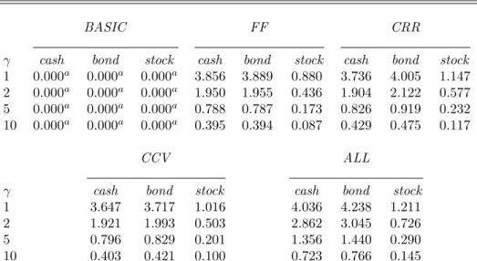
(15) term returns are largely predictable, excess bond returns are more difficult to forecast, and excess stock returns are even more difficult to predict. Overall, the returns analysis reveals four important implications for portfolio allocations. First, both the ¯ 2 statistics indicate that the baseline specification is rejected. significance levels of dynamic feedbacks and R This finding unambiguously refutes the notion that investment opportunities are constant, and thus, that portfolio allocations should be purely tactical. Second, the significance levels of dynamic feedbacks show that certain variable groups affect the return variables for all alternative factor sets. This result accords with the empirical asset-pricing literature documenting the predictability of returns, and confirms that investment opportunities are time-varying. Third, the significance levels of innovation correlations highlight several co-movements between the return and factor variables. These co-movements are necessary conditions for dynamic hedging strategies, which accords with the fact that the empirical shares of cash, bonds, and stocks ¯ 2 statistics are very close feature pronounced fluctuations through time (see Figures 1 and 2). Fourth, the R across the various alternative factor sets. Consequently, the identification of the most influential factor set for portfolio allocations remains an open question. For this reason, rather than focusing on a single factorial specification, we next perform our portfolio analysis for every factor sets.. 3. Portfolio Analysis. This section compares the empirical and predicted portfolio shares. For this purpose, the empirical shares are constructed for cash, bonds, and stocks by evaluating the definition (6) from a measure of (financial) wealth corresponding to the sum of the values of the three assets and from quarterly aggregate U.S. data covering the post-war period (see the Data Appendix). Table 3 reports descriptive statistics for empirical shares. Note that both the empirical shares for cash and stocks display large means and volatilities, whereas the empirical share for bonds has much lower average and standard deviation. Also, the empirical share for cash exhibits negative co-movements with the empirical share for bonds as well as the one for stocks, while the empirical shares for bonds and stocks are positively correlated.. 12.

(16) [ Insert Table 3 here ] In principle, these empirical shares should accord with the measures of return variables used in the VAR process (4). This is verified by comparing the implicit returns induced by the empirical shares to empirical returns. The (nominal, quarterly) implicit returns are obtained through the following expression:. ri,t+1 =. wi,t+1 − 1, αi,t (wt − ct ). (10). where the variables on the right-hand side are evaluated from the empirical shares and quarterly nominal observations on consumption, asset value, and wealth. Equation (10) can be reconciliated with the investor’s budget constraint (2). To see this, isolate wi,t+1 , sum over all assets, and use (3) to yield £Pnr. i=1 (1. Pnr i=1. wi,t+1 =. ¤ £ ¤ Pnr + ri,t+1 )αi,t (wt − ct ) = 1 + r1,t+1 + i=2 αi,t xri,t+1 (wt − ct ), or equivalently, wt+1 = (1 +. rp,t+1 )(wt − ct ). Table 3 also presents summary statistics for implicit and empirical returns. Interestingly, the implicit and empirical returns on cash, bonds, and stocks all feature means and volatilities that are almost identical. In addition, the implicit and empirical excess returns on bonds and stocks are characterized by Sharpe ratios that are almost identical. Overall, these findings suggest that our measures of empirical shares are consistent with our measures of empirical returns. The predicted portfolio shares are constructed by evaluating the decision rules (8) and (9) for quarterly post-war U.S. data. To this end, we evaluate the coefficients of the decision rules from specific values for the parameters of the VAR process (4) and investor’s preferences (1). For the VAR parameters, we use the OLS estimates presented previously for the various specifications. The baseline (alternative) specification permits us to test constant (time-varying) investment opportunity sets obtained from Φ1 = 0 (Φ1 6= 0). For the preference parameters, we calibrate the time discount factor to the standard value of δ = 0.979, which corresponds to a quarterly (net) discount rate of 2.1 percent. We also set the elasticity of inter-temporal substitution to the single value ψ = 1/2, given that alternative values have no effect on the predicted portfolio shares. A similar invariance result is obtained for the cases of single risky asset and state variable (Campbell. 13.

(17) and Viceira, 1999), many risky assets and a unique state variable (Normandin and St-Amour, 2002), and several risky assets and state variables (Campbell et al., 2003). We further fix the relative risk aversion to the values γ = 1, 2, 5, and 10. These calibrations are reasonable given the widely accepted beliefs about attitudes towards risk (Mehra and Prescott, 1985). Moreover, the different calibrations allow us to test myopic (non-myopic) portfolio rules induced by γ = 1 (γ > 1). Finally, we perform formal statistical tests to confront the empirical and predicted portfolio shares by focusing on their means, volatilities, and co-movements. These tests rely on χ2 (1)-distributed Wald statistics that take into account the uncertainty related to the estimates of the VAR parameters, using the δ-method. Table 4 presents the averages of the predicted portfolio shares and the levels of significance of the associated statistical test. Tables 5 and 6 report similar information, but for the standard deviations and correlations of the predicted shares.. BASIC. A non-conservative investor (γ = 1) takes, on average, a short position on cash, and long positions. on bonds and stocks. Thus, the investor borrows a sizable share of his wealth in the less risky asset to finance large holdings in bonds and stocks. This occurs because the Sharpe ratios, computed from excess returns, are positive for both bonds and stocks (see Table 3). In addition, the share invested in stocks is always larger than that held in bonds. This is due to the notion that stocks display the largest Sharpe ratio. In contrast, a conservative investor (γ > 1) takes long positions in all assets, as the share in cash increases and those in bonds and stocks decrease when the relative risk aversion increases. This is explained by the tactical portfolio allocation: a larger demand for cash allows the investor to diversify away the risk, given that the unexpected benchmark return is negatively correlated with unanticipated excess returns on bonds and on stocks (see Table 2). However, there is no such increase in the demand for bonds, since unanticipated excess returns on bonds and stocks are positively correlated. For almost all reasonable values of relative risk aversion, the averages of the predicted portfolio shares for cash and stocks are significantly different from those of the empirical shares. Furthermore, the zero standard deviations and correlations of the predicted shares are always statistically different from their empirical. 14.

(18) counterparts. In sum, these test results indicate that the investor’s tactical behavior is strongly rejected by the data.. FF. A myopic investor (γ = 1) takes, on average, a short position on cash, and long positions on bonds. and stocks. This myopic behavior is similar than the tactical behavior just explained for the BASIC case. This arises because both the myopic and tactical portfolio allocations abstract from hedging strategies. From a statistical perspective, the myopic behavior predicts a mean for the share of stocks and a correlation between the shares of cash and bonds that are significantly different from there empirical counterparts. In addition, all the means (in absolute values) and volatilities, as well as most correlations (in absolute values) of the predicted shares largely numerically over-state those of the empirical shares. These findings are clearly not in favor of the myopic behavior. A non-myopic investor (γ > 1) takes long positions in all assets, as the share in cash increases and those in bonds and stocks decrease when the relative risk aversion increases. Interestingly, the strategic behavior of the non-myopic investor implies that the decrease in the share of stocks (bonds) is less (more) pronounced, relative to that found from the tactical behavior. This suggests that stocks are better dynamic hedges against adverse changes in investment opportunities. Statistically, the strategic behavior predicts means and volatilities that are never significantly different from those found in the data. This behavior further predicts correlations for the shares of cash and of bonds with that of stocks that are never statistically different from the empirical ones, whereas the predicted correlations between the shares of cash and bonds are significantly different from the data, except for the case where the relative risk aversion is γ = 10. Furthermore, it is worth stressing that the predicted shares exhibit the appropriate signs and magnitudes for the means when γ = 2 and 5 for all assets, and adequate volatilities when γ = 5 and 10 for stocks. In addition, the predicted correlations for the share of cash with that of bonds and of stocks display the correct signs, regardless of the value of γ. Overall, these results provide empirical support for the strategic portfolio allocation obtained by combining reasonable degrees of risk aversions with the F F set of factors.. 15.

(19) CRR. As above, a myopic investor (γ = 1) takes, on average, a short position on cash, and long positions. on bonds and stocks. Also, the predicted mean for the share of stocks and correlation between the shares of cash and bonds are statistically at odds with the data. Finally, all the predicted means (in absolute values) and volatilities over-estimate the empirical ones, while the predicted correlations often display the wrong signs. Again, these findings indicate that the myopic behavior is refuted. A non-myopic investor (γ > 1) usually takes long positions in cash and stocks, but short positions in bonds. Also, the strategic behavior induced by the CRR factor set implies that the fall in demand for bonds is so pronounced that it drives the share for bonds to be negative, in contrast to that obtained from the F F case. The test results reveal that the strategic behavior associated with the CRR specification predicts means and volatilities that are never statistically different from the empirical ones. Also, the predicted correlations for the shares of cash and of bonds with that of stocks are never statistically different from the empirical ones. However, the predicted correlations between the shares of cash and bonds are always significantly different from the data. Moreover, the predicted means for the share of bonds and correlations between the shares of cash and stocks display the wrong signs, for almost all reasonable values of γ. In this sense, the strategic portfolio allocation derived from the CRR specification is performing worse than the one related to F F factor set.. CCV. A myopic investor (γ = 1) takes, on average, identical asset positions as those explained previously.. Also, this myopic behavior features similar statistical and numerical properties as those described above. Consequently, the myopic behavior is once again inconsistent with the data. A non-myopic investor (γ > 1) takes similar asset positions as those explained for the CRR specification. Also, the strategic behavior induced by the CCV factor set exhibits similar statistical and numerical results to those reported for the CRR case. In particular, the predicted means for the share of bonds and correlations between the shares of cash and stocks systematically display the wrong signs. Hence, the strategic portfolio. 16.

(20) allocation derived from the CCV specification is also less attractive than the one associated with the F F factor set.. ALL. A myopic investor (γ = 1) is characterized by a behavior that is numerically and statistically close to. that documented above. As a result, the myopic behavior is once more time at odds with the data. Finally, a non-myopic investor (γ > 1) has a strategic behavior that numerically and statistically parallels those discussed for the CRR and CCV specifications. For this reason, the strategic portfolio allocation derived from the ALL factor set is less appropriate than the one associated with the F F case. In sum, the portfolio analysis highlights two key findings for the assessment of portfolio allocations. First, the various moments of the empirical portfolio shares are never replicated from the baseline specification, nor from the combinations of any alternative factor sets with a relative risk aversion of one. This empirical evidence clearly refutes both tactical and myopic investment behaviors. Second, the properties of the empirical portfolio shares are best explained by combining the F F factors with reasonable values of relative risk aversion larger than unity. For example, this case yields predictions that are almost always statistically appropriate, and that exhibit the correct signs and numerical magnitudes. In particular, this is the only case for which the predicted means for the share of bonds and correlations between the shares of cash and stocks display the adequate signs. For these reasons, the F F case is our preferred specification. Moreover, this specification with the relevant values of relative risk aversion provides additional empirical support for strategic portfolio allocations. To reach a more definitive conclusion, however, it is necessary to assess whether this environment also implies a consumption behavior that accords with the data. We now turn to this issue.. 4. Consumption Analysis. In this section, we verify whether the empirical and predicted consumption shares are the same. The empirical share is constructed by evaluating the definition (5) from quarterly aggregate U.S. data for the. 17.

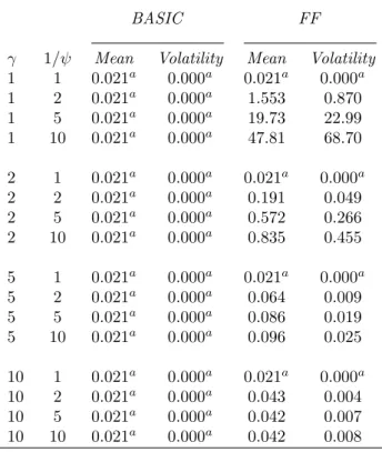
(21) post-war period (see the Data Appendix). This share exhibits a mean of 0.135 and a standard deviation of 0.026. The predicted consumption shares are constructed by evaluating the decision rule (7) for quarterly postwar U.S. data. To do so, we fix the VAR parameters to their OLS estimates. The baseline (alternative) specification enables us to test constant (time-varying) investment opportunity sets derived from Φ1 = 0 (Φ1 6= 0), where the consumption share is fixed (variable). For briefness, we limit our analysis of the alternative VAR processes to the F F case, i.e. our preferred specification for portfolio shares. As before, we use the standard calibration δ = 0.979 and the reasonable values γ = 1, 2, 5, and 10. This time, however, we consider the following calibrations ψ = 1, 1/2, 1/5 and 1/10, given that the elasticity of inter-temporal substitution is known to affect the predicted consumption shares (Campbell and Viceira 1999; Normandin and St-Amour 2002). The different calibrations permit us to study consumption shares predicted by separable (non-separable) preferences obtained from γ = ψ −1 (γ 6= ψ −1 ). In addition, we can test myopic (non-myopic) consumption rules induced by ψ = 1 (ψ < 1), where the consumption share is fixed (variable). Again, we apply formal statistical tests to confront the empirical and predicted consumption shares by focusing on their means and volatilities. Table 7 presents the statistics for the predicted consumption shares and the levels of significance of the associated tests.. BASIC. The consumer always spends a constant fraction of his wealth, where this proportion is equal to. the reasonable calibration for the quarterly (net) discount rate. This is a consequence of the absence of changes in investment opportunities, imposed by the BASIC specification. From a statistical perspective, the predicted means and volatilities are systematically significantly different from the empirical counterparts.. FF. A myopic consumer (ψ = 1) has an identical spending pattern than that observed for the BASIC. specification. This time, however, this is explained by the exact cancellation of the inter-temporal substitution and income effects associated with changes in investment opportunities. Statistically, the predicted means and volatilities are always significantly at odds with the data.. 18.

(22) A non-myopic consumer (ψ < 1) has consumption shares that always exhibit positive means and volatilities. In addition, these predicted means and volatilities decrease in relative risk aversion. This suggests that a highly risk-averse investor prefers to reduce his consumption exposure to changes in the states. Statistically, the non-myopic behavior predicts means and volatilities that are never significantly different from those found in the data. However, the predicted means and volatilities greatly numerically over-state the empirical ones, as long as γ = 1. In contrast, the predicted means and volatilities exhibit the appropriate magnitudes for the separable preferences γ = ψ −1 = 2 and non-separable preferences γ = 5 and ψ −1 = 10. Thus, combining these reasonable calibrations for the preference parameters with the estimates for the F F specification parameters yields predictions that accord with the data. In brief, the consumption analysis reveals two important results for the evaluation of portfolio allocations. First, the moments of the empirical consumption share are never reproduced from the BASIC specification, nor from the combination of the F F factors with a relative risk aversion of one. These facts confirm the rejection of both tactical portfolio allocations and myopic investment behaviors. Second, the properties of the empirical consumption share can be recovered by combining the F F specification with reasonable values of relative risk aversion larger than unity. Interestingly, this accords with our earlier findings in favor of strategic portfolio allocations. Overall, this paper has highlighted the important time variation in U.S. aggregate portfolio allocations. To analyze this, we first used flexible descriptions of preferences and investment opportunities to derive optimal decision rules that nest tactical, myopic, and strategic portfolio allocations. We then compared these rules to the data through formal statistical analysis. Our main results revealed that i) purely tactical and myopic investment behaviors are unambiguously rejected, ii) strategic portfolio allocations are strongly supported, and iii) the Fama-French factors best explain empirical portfolio shares.. 19.

(23) A. Data Appendix. This appendix describes the quarterly U.S. data covering the 1952:II-2000:IV period.. Portfolio and Consumption Variables cash: portfolio share in cash. This corresponds to the value of cash relative to wealth. The value of cash is measured by the seasonally unadjusted U.S. nominal checkable deposits and currency plus nominal time and saving deposits (Source: Board of Governors of the Federal Reserve Bank, Balance Sheet of Households and Nonprofit Organizations).. bond:. portfolio share in bonds. This is the value of bonds divided by wealth. The value of bonds is captured. by the seasonally unadjusted nominal U.S. government securities (Source: Board of Governors of the Federal Reserve Bank, Balance Sheet of Households and Nonprofit Organizations).. stock: portfolio share in stocks. This is the value of stocks normalized by wealth. The value of stocks corresponds to the seasonally unadjusted U.S. nominal corporate equities (Source: Board of Governors of the Federal Reserve Bank, Balance Sheet of Households and Nonprofit Organizations).. cons:. consumption share. This is the value of consumption divided by wealth. The value of consumption. is measured by the seasonally adjusted U.S. nominal private consumption expenditures on nondurable goods and services (Source: U.S. Department of Commerce, Bureau of Economic Analysis).. wealth:. This is the sum of the values of cash, bonds, and stocks.. Return Variables rtb,t : ex post real Treasury bill rate. This is the difference between the quarterly (annualized) nominal return on 90-day U.S. Treasury bill (Source: Center for Research in Security Prices) and the inflation rate.. 20.

(24) xrb,t : excess bond return. This is the difference between the quarterly (annualized) nominal return on fiveyear U.S. Treasury bonds (Source: Center for Research in Security Prices) and the quarterly (annualized) nominal return on 90-day U.S. Treasury bill.. xrs,t : excess stock return. This is the difference between the quarterly (annualized) nominal value-weighted return (including dividends) on the NYSE, NASDAQ, and AMEX markets (Source: Center for Research in Security Prices) and the quarterly (annualized) nominal return on 90-day U.S. Treasury bill.. Goods-Market Variables inft : inflation rate. This is the quarterly (annualized) growth rate of the seasonally adjusted U.S. gross domestic product implicit deflator (Source: U.S. Department of Commerce, Bureau of Economic Analysis).. prodt : production growth. This is the difference between the quarterly (annualized) growth rate of the seasonally adjusted U.S. nominal gross domestic product (Source: U.S. Department of Commerce, Bureau of Economic Analysis) and the inflation rate.. Equity-Market Variables smbt :. (Small Minus Big): excess small-portfolio return. This is the difference between the quarterly (annu-. alized) average return on three small U.S. portfolios and the quarterly (annualized) average return on three big U.S. portfolios (Source: http://mba.tuck.dartmouth.edu/pages/faculty/ken.french/data library.html).. hmlt : (High Minus Low): excess value-portfolio return. This is the difference between the quarterly (annualized) average return on two value U.S. portfolios and the quarterly (annualized) average return on two growth U.S. portfolios (Source: http://mba.tuck.dartmouth.edu/pages/faculty/ken.french/data library.html).. dt − pt : dividend-price ratio. This is the difference between the logarithm of the dividend payout and the logarithm of the price index. The dividend payout and the price index are calculated from the value-weighted. 21.

(25) returns (including and excluding dividends) on the NYSE, NASDAQ, and AMEX markets (Source: Center for Research in Security Prices).. Bond-Market Variables termt : excess long-term government-bond return. This term structure of interest rates is the difference between the quarterly (annualized) interest rate on five-year zero-coupon U.S. government bonds (Source: Center for Research in Security Prices) and the quarterly (annualized) nominal return on 90-day U.S. Treasury bill.. deft :. excess long-term corporate-bond return. This bond default premium is the difference between the. quarterly (annualized) nominal yield on Baa U.S. corporate bonds (Source: Moody’s Investors Service) and the quarterly (annualized) nominal return on 90-day U.S. Treasury bill.. 22.

(26) 23. B. 0.000. 0.000. 0.011. 0.017a. 0.000. 0.062a. xrs,t+1. FF. 0.065 [1.452]. [5.998a ]. 0.590. 0.036. 2.420a -0.308 [3.760a ]. 0.116. 2.987 0.948 [0.950]. [1.929c ]. [2.501b ]. 0.114 0.223a [3.731a ]. [2.590b ]. -0.289b -0.122. -1.013a -0.323. 0.384b. -0.013 -0.040a. 0.003 [71.83a ]. -0.067 -0.050b. -0.013. -0.028. 1.382a. 0.705a. 0.011. xrs,t+1. -0.021. xrb,t+1. -0.001. rtb,t+1. CRR. 0.589. 0.112. 0.063. Bond-Market Variables 0.268b 2.427a -4.343 -0.057 -0.579 10.40a [2.369b ] [2.950b ] [3.722a ]. Stock-Market Variables. [7.698a ]. 0.597. [5.181a ]. 0.248a. -0.006b [3.112b ]. 0.162a [10.88a ]. [51.92a ] Goods-Market Variables -0.013 -0.382b 0.032 0.147b -0.150 -5.654a [2.065c ] [1.558] [5.375a ]. -0.002 0.007a [89.42a ]. 0.016. 0.799a. -0.076 -0.063a. Return Variables 1.573a -3.833a. rtb,t+1 -0.024a. xrs,t+1 0.115b. -0.001. xrb,t+1. -0.058 [2.174b ]. -0.002 0.006b. 0.823a. -0.003. rtb,t+1. 0.107. [4.608a ]. 1.897a. 0.026 [1.037]. -0.332 [0.698]. [7.531a ]. -0.066 -0.070a. 1.333a. 0.076. xrb,t+1. CCV. Table 1: Returns Analysis: Estimates of the Parameters. 0.057. [0.112]. 0.844. 0.163a [5.062a ]. -2.877a [6.419a ]. [1.595]. -0.037. -0.305 0.439a. 0.715a. xrs,t+1. 0.597. 0.317a -0.063 [3.313a ]. -0.017 -0.033b -0.004 [2.281b ]. -0.007 0.180a [2.682b ]. [52.28a ]. -0.001 0.006c. 0.821a. -0.019c. rtb,t+1. ALL. 0.121. 2.614a -0.555 [3.434a ]. -0.298b -0.133 0.033 [1.632]. -0.328c -0.197 [1.158]. [6.508a ]. -0.092 -0.053b. 1.545a. 0.113. xrb,t+1. 0.107. -4.174 10.93a [4.375a ]. -0.918b -0.641c 0.210a [4.083a ]. 0.262 -6.516a [6.958a ]. [2.240b ]. -0.057. -0.053. -4.013a. 0.850a. xrs,t+1. Note: Entries are the OLS parameter estimates of the return equations for the different specifications of the VAR process. Numbers in brackets are the F statistics of the test that the estimates associated with the return variables, the goods-market variables, the stock-market variables, or the bond-market variables are jointly null. a, b, and c indicate that the estimates are individually or jointly significant at the 5, 10, and 15 percent levels.. ¯2 R. termt deft. smbt hmlt dt − pt. prodt inft. rtb,t xrb,t xrs,t. cst. BASIC. xrb,t+1. rtb,t+1. Tables.

(27) 24. -0.020 -0.020 [0.155]. BASIC. 0.197a [7.607a ]. -0.020. xrb,t+1. [7.607a ]. -0.020 0.197a. xrs,t+1. FF. -0.015 0.048 [0.491] 0.147a 0.811a [131.8a ]. [1.845] -0.330a -0.271a [35.37a ]. 0.191a [37.96a ]. -0.399a. xrb,t+1. -0.086 0.046. -0.399a -0.096 [32.67a ]. rtb,t+1. 0.080 0.056 [1.850]. [60.71a ]. 0.416a -0.374a. [8.865a ]. -0.096 0.191a. xrs,t+1. CRR. Bond-Market Variables -0.312a 0.147a 0.025 -0.287a 0.824a 0.126b a a [34.86 ] [141.7 ] [3.201]. Stock-Market Variables. 0.216a [37.81a ]. CCV. 0.126b [3.080b ]. [16.32a ]. 0.020 [0.077]. -0.132b [3.380b ]. 0.197a [34.23a ]. -0.371a. xrb,t+1. -0.290a. 0.124b [2.983b ]. -0.761a [112.3a ]. rtb,t+1. [9.462a ]. -0.046 0.216a. xrs,t+1. Goods-Market Variables 0.389a -0.222a 0.009 -0.767a -0.119b -0.072 a a [143.5 ] [12.31 ] [1.021]. Return Variables -0.385a. xrb,t+1. -0.371a -0.029 [26.87a ]. -0.385a -0.046 [29.17a ]. rtb,t+1. [0.770]. 0.063. 0.059 [0.675]. -0.098 [1.863]. [7.692a ]. -0.029 0.197a. xrs,t+1. -0.297a -0.316a [36.48a ]. -0.080 0.044 0.097 [3.443]. 0.405a -0.766a [145.7a ]. -0.404a -0.047 [32.09a ]. rtb,t+1. ALL. 0.140b 0.825a [135.8a ]. -0.020 0.056 -0.038 [0.966]. -0.217a -0.096 [10.923a ]. 0.186a [38.38a ]. -0.404a. xrb,t+1. -0.001 0.105c [2.139]. 0.420a -0.387a 0.026 [63.41a ]. 0.035 -0.046 [0.648]. [7.140a ]. -0.047 0.186a. xrs,t+1. Note: Entries are the cross-correlations between the innovations of return variables and other state variables for the different specifications of the VAR process. Numbers in brackets are the χ2 statistics of the Box-Pierce test that the cross-correlations between the innovations of each return variable and the other return variables, the goods-market variables, the stock-market variables, or the bond-market variables are jointly null. a, b, and c indicate that the cross-correlations are individually or jointly significant at the 5, 10, and 15 percent levels.. term def. smb hml d−p. prod inf. rtb xrb xrs. rtb,t+1. Table 2: Returns Analysis: Cross-Correlations of the State-Variable Innovations.

(28) Table 3: Portfolio Analysis: Empirical Shares and Returns Shares Volatility. Mean. Empirical. cash 0.458. bond 0.092. stock 0.450. cash 0.122. bond 0.034. stock 0.109. Returns Volatility. Mean. Empirical Implicit. Co-movement cash -0.497. bond -0.963. stock 0.246. Sharpe Ratio. cash. bond. stock. cash. bond. stock. bond. stock. 0.013 0.017. 0.016 0.015. 0.029 0.024. 0.007 0.009. 0.029 0.028. 0.080 0.090. 0.152 0.119. 0.355 0.303. Note: Shares: Entries are the means, standard deviations, and cross-correlations of the empirical portfolio shares in cash, bond, and stock. Returns: Entries are the means, standard deviations, and Sharpe ratios for the empirical and implicit returns. The means and standard deviations are computed from quarterly nominal returns for cash, bonds, and stocks. The Sharpe ratios are calculated from quarterly (annualized) excess returns for bonds and stocks. These ratios correspond to the sum of the mean and half of the variance of the excess return, normalized by its standard deviation.. Table 4: Portfolio Analysis: Mean BASIC γ 1 2 5 10. cash -0.774a 0.111 0.642c 0.819a. bond 0.735 0.369 0.149 0.076. FF stock 1.039a 0.520 0.209a 0.105a. cash -0.915 0.232 0.688 0.796. bond 0.834 0.191 0.058 0.058. CRR stock 1.080a 0.577 0.255 0.146. CCV γ 1 2 5 10. cash -0.883 3.726 3.823 2.539. bond 0.796 -3.469 -3.109 -1.657. cash -0.862 0.394 0.904 0.694. bond 0.752 -0.048 -0.177 0.167. stock 1.110c 0.654 0.273 0.139. ALL stock 1.087a 0.743 0.285 0.119. cash -0.416 5.411 7.391 5.748. bond -0.562 -6.022 -7.111 -5.078. stock 1.977 1.611 0.720 0.330. Note: Entries are the means of the predicted portfolio shares. The means of the empirical portfolio shares are 0.458 for cash, 0.092 for bond, and 0.450 for stock. a, b, and c indicate that the difference between the predicted and empirical means is significant at the 5, 10, and 15 percent levels. These tests use the variance of the difference, which is computed as D0 ΞD — where D is the vector of numerical derivatives of the difference with respect to the parameters of the VAR process, and Ξ is the covariance matrix of these parameters.. 25.

(29) Table 5: Portfolio Analysis: Volatility BASIC γ 1 2 5 10. cash 0.000a 0.000a 0.000a 0.000a. bond 0.000a 0.000a 0.000a 0.000a. FF stock 0.000a 0.000a 0.000a 0.000a. cash 3.856 1.950 0.788 0.395. bond 3.889 1.955 0.787 0.394. CRR stock 0.880 0.436 0.173 0.087. CCV γ 1 2 5 10. cash 3.647 1.921 0.796 0.403. bond 3.717 1.993 0.829 0.421. cash 3.736 1.904 0.826 0.429. bond 4.005 2.122 0.919 0.475. stock 1.147 0.577 0.232 0.117. ALL stock 1.016 0.503 0.201 0.100. cash 4.036 2.862 1.356 0.723. bond 4.238 3.045 1.440 0.766. stock 1.211 0.726 0.290 0.145. Note: Entries are the standard deviations of the predicted portfolio shares. The standard deviations of the empirical portfolio shares are 0.122 for cash, 0.034 for bond, and 0.109 for stock. a, b, and c indicate that the difference between the predicted and empirical standard deviations is significant at the 5, 10, and 15 percent levels. These tests use the variance of the difference, which is computed as D0 ΞD — where D is the vector of numerical derivatives of the difference with respect to the parameters of the VAR process, and Ξ is the covariance matrix of these parameters.. 26.

(30) 27. cash–bond 0.000a 0.000a 0.000a 0.000a. cash–bond -0.962a -0.968a -0.970a -0.971c. cash–stock 0.000a 0.000a 0.000a 0.000a. cash–stock -0.070 0.015 0.042 0.051. CCV. bond–stock 0.000a 0.000a 0.000a 0.000a. bond–stock -0.204 -0.267 -0.283 -0.287. cash–bond -0.974a -0.975a -0.976a -0.976. cash–stock -0.076 -0.098 -0.114 -0.120. FF. cash–bond -0.958a -0.972a -0.980a -0.983a. bond–stock -0.151 -0.125 -0.106 -0.100. cash–stock 0.021 0.133 0.193 0.210. ALL. cash–bond -0.959a -0.965a -0.970b -0.972c. bond–stock -0.306 -0.364 -0.383 -0.387. cash–stock 0.089 0.248 0.283 0.286. CRR bond–stock -0.369 -0.494 -0.507 -0.503. Note: Entries are the correlations between the predicted portfolio shares. The correlations of the empirical portfolio shares are -0.497 between cash and bond, -0.963 between cash and stock, and 0.246 between bond and stock. a, b, and c indicate that the difference between the predicted and empirical correlations is significant at the 5, 10, and 15 percent levels. These tests use the variance of the difference, which is computed as D0 ΞD — where D is the vector of numerical derivatives of the difference with respect to the parameters of the VAR process, and Ξ is the covariance matrix of these parameters.. γ 1 2 5 10. γ 1 2 5 10. BASIC. Table 6: Portfolio Analysis: Co-movement.

(31) Table 7: Consumption Analysis: Mean and Volatility BASIC. FF. γ 1 1 1 1. 1/ψ 1 2 5 10. Mean 0.021a 0.021a 0.021a 0.021a. Volatility 0.000a 0.000a 0.000a 0.000a. Mean 0.021a 1.553 19.73 47.81. Volatility 0.000a 0.870 22.99 68.70. 2 2 2 2. 1 2 5 10. 0.021a 0.021a 0.021a 0.021a. 0.000a 0.000a 0.000a 0.000a. 0.021a 0.191 0.572 0.835. 0.000a 0.049 0.266 0.455. 5 5 5 5. 1 2 5 10. 0.021a 0.021a 0.021a 0.021a. 0.000a 0.000a 0.000a 0.000a. 0.021a 0.064 0.086 0.096. 0.000a 0.009 0.019 0.025. 10 10 10 10. 1 2 5 10. 0.021a 0.021a 0.021a 0.021a. 0.000a 0.000a 0.000a 0.000a. 0.021a 0.043 0.042 0.042. 0.000a 0.004 0.007 0.008. Note: Entries are means and standard deviations of the predicted consumption share. The mean and standard deviation of the empirical consumption share are 0.135 and 0.026. a, b, and c indicate that the difference between the predicted and empirical moments is significant at the 5, 10, and 15 percent levels. These tests use the variance of the difference, which is computed as D0 ΞD — where D is the vector of numerical derivatives of the difference with respect to the parameters of the VAR process, and Ξ is the covariance matrix of these parameters.. 28.

(32) C. Figures Figure 1: Empirical Portfolio Shares 0.7 Cash Bonds Stocks 0.6. 0.5. 0.4. 0.3. 0.2. 0.1. 0 1950. 1960. 1970. 1980. 1990. 2000. 2010. Note: The solid [dotted] (dashed) lines represent the empirical portfolio shares of cash [bonds] (stocks). Each empirical share is measured as the value of the asset holdings relative to wealth, where wealth is the sum of the values of holdings of cash, bonds, and stocks (See the Data Appendix).. 29.

(33) Figure 2: Ratio of Empirical Portfolio Shares 0.55 Bonds / Stocks 0.5. 0.45. 0.4. 0.35. 0.3. 0.25. 0.2. 0.15. 0.1. 0.05 1950. 1960. 1970. 1980. 1990. 2000. Note: The solid line represents the ratio of the empirical share of bonds to that of stocks.. 30. 2010.

(34) References Campbell, J. Y., Chan, Y. L., and Viceira, L. M. (2003), “A Multivariate Model of Strategic Asset Allocation,” Journal of Financial Economics, 67, 41–80. Campbell, J. Y. and Koo, H. K. (1997), “A Comparison of Numerical and Analytical Approximate Solutions to an Intertemporal Consumption Choice Problem,” Journal of Economic Dynamics and Control, 21, 273–295. Campbell, J. Y. and Viceira, L. M. (1999), “Consumption and Portfolio Decisions when Expected Returns are Time Varying,” Quarterly Journal of Economics, 114, 433–495. Chen, N.-F., Roll, R., and Ross, S. A. (1986), “Economic Forces and the Stock Market,” Journal of Business, 59, 383–403. Epstein, L. G. and Zin, S. E. (1989), “Substitution, Risk Aversion and the Temporal Behavior of Consumption and Asset Returns: A Theoretical Framework,” Econometrica, 57, 937–969. Fama, E. F. and French, K. R. (1993), “Common Risk Factors in the Returns on Stocks and Bonds,” Journal of Financial Economics, 33, 3–56. Ferson, W. E. and Harvey, C. R. (1999), “Conditionaing Variables and the Cross Section of Stock Returns,” Journal of Finance Papers and Proceedings, 54, 1325–1360. Giovannini, A. and Weil, P. (1989), “Risk-Aversion and Inter-Temporal Substitution in the Capital Asset Pricing Model,” Working Paper 2824, National Bureau of Economic Research. Mehra, R. and Prescott, E. C. (1985), “The Equity Premium: A Puzzle,” Journal of Monetary Economics, 15, 145–161. Normandin, M. and St-Amour, P. (2002), “Canadian Consumption and Portfolio Shares,” Canadian Journal of Economics, 35, 737–756. Weil, P. (1990), “Non-expected Utility in Macroeconomics,” Quarterly Journal of Economics, 105, 29–42. 31.

(35)