The Road to Power: Partisan Loyalty and the Centralized Provision of Local Infrastructure

Texte intégral

(1)2009s-46. The Road to Power: Partisan Loyalty and the Centralized Provision of Local Infrastructure Marcelin Joanis. Série Scientifique Scientific Series. Montréal Novembre 2009. © 2009 Marcelin Joanis. Tous droits réservés. All rights reserved. Reproduction partielle permise avec citation du document source, incluant la notice ©. Short sections may be quoted without explicit permission, if full credit, including © notice, is given to the source..

(2) CIRANO Le CIRANO est un organisme sans but lucratif constitué en vertu de la Loi des compagnies du Québec. Le financement de son infrastructure et de ses activités de recherche provient des cotisations de ses organisations-membres, d’une subvention d’infrastructure du Ministère du Développement économique et régional et de la Recherche, de même que des subventions et mandats obtenus par ses équipes de recherche. CIRANO is a private non-profit organization incorporated under the Québec Companies Act. Its infrastructure and research activities are funded through fees paid by member organizations, an infrastructure grant from the Ministère du Développement économique et régional et de la Recherche, and grants and research mandates obtained by its research teams. Les partenaires du CIRANO Partenaire majeur Ministère du Développement économique, de l’Innovation et de l’Exportation Partenaires corporatifs Banque de développement du Canada Banque du Canada Banque Laurentienne du Canada Banque Nationale du Canada Banque Royale du Canada Banque Scotia BMO Groupe financier Caisse de dépôt et placement du Québec DMR Fédération des caisses Desjardins du Québec Gaz Métro Hydro-Québec Industrie Canada Investissements PSP Ministère des Finances du Québec Power Corporation du Canada Raymond Chabot Grant Thornton Rio Tinto State Street Global Advisors Transat A.T. Ville de Montréal Partenaires universitaires École Polytechnique de Montréal HEC Montréal McGill University Université Concordia Université de Montréal Université de Sherbrooke Université du Québec Université du Québec à Montréal Université Laval Le CIRANO collabore avec de nombreux centres et chaires de recherche universitaires dont on peut consulter la liste sur son site web. Les cahiers de la série scientifique (CS) visent à rendre accessibles des résultats de recherche effectuée au CIRANO afin de susciter échanges et commentaires. Ces cahiers sont écrits dans le style des publications scientifiques. Les idées et les opinions émises sont sous l’unique responsabilité des auteurs et ne représentent pas nécessairement les positions du CIRANO ou de ses partenaires. This paper presents research carried out at CIRANO and aims at encouraging discussion and comment. The observations and viewpoints expressed are the sole responsibility of the authors. They do not necessarily represent positions of CIRANO or its partners.. ISSN 1198-8177. Partenaire financier.

(3) The Road to Power: Partisan Loyalty and the Centralized Provision of Local Infrastructure Marcelin Joanis*. Résumé / Abstract Cet article développe un modèle dynamique simple de vote probabiliste dans lequel un gouvernement répartit un budget fixe entre des circonscriptions électorales qui diffèrent selon leur degré de loyauté au parti au pouvoir. Le modèle prédit que la répartition géographique des dépenses dépend de la manière dont le gouvernement assure l’équilibre entre des considérations de long terme de type « machine électorale » et des considérations plus immédiates de victoire dans les circonscriptions pivot. Des résultats empiriques obtenus à partir d’un panel de circonscriptions électorales au Québec montrent que les circonscriptions qui sont loyales au parti au pouvoir reçoivent plus que leur part de dépenses, particulièrement à l’approche d’une élection, contrairement à la vision théorique traditionnelle prédisant plus de dépenses dans les circonscriptions pivot. Mots clés : loyauté partisane, électeurs pivot, concurrence électorale, biens publics locaux, clientélisme politique, relations de long terme.. This paper sets out a simple dynamic probabilistic voting model in which a government allocates a fixed budget across electoral districts that differ in their loyalty to the ruling party. The model predicts that the geographic pattern of spending depends on the way the government balances long-run ‘machine politics’ considerations and the more immediate concern to win over swing voters. Empirical results obtained from a panel of electoral districts in Québec provide robust evidence that districts which display loyalty to the incumbent government receive disproportionately more spending, especially close to an election, at odds with the standard ‘swing voter’ view. Keywords: partisan loyalty, swing voters, political competition, local public goods, distributive politics, long-run relationships. Codes JEL : D72, H41, H54 *. I thank Robert McMillan, Michael Smart, Michael Baker, Adonis Yatchew, François Vaillancourt, André Blais, Timothy Besley, Brian Knight, and an anonymous referee for their suggestions. I also thank seminar participants at Université de Sherbrooke, University of Toronto, Industry Canada, U. of Oklahoma, CRA International, U. of Louisville, University of Kentucky, UC-Merced, PPIC, SUNY-Albany, CEA (Montréal 2006), SCSE (Montréal 2006) and PCS (Amsterdam 2007). I am most grateful to Benoît Méthot for his input in the early stages of this research. All remaining errors are mine. Contact address: Université de Sherbrooke, Faculté d'administration, 2500, boul. de l'Université, Sherbrooke (Québec), J1K 2R1, email: marcelin.joanis@usherbrooke.ca..

(4) “... the new road turns from pavement into gravel (‘Must’ve elected the wrong guy last time around,’David says...)” –Margaret Atwood, Surfacing, 1972, p. 18. 1. Introduction. Spectacular events involving aging public infrastructures, such as the Minneapolis bridge collapse in the summer of 2007, inevitably spark debates in the popular press about electoral misallocation of infrastructure spending.1 This is not surprising since public infrastructures such as roads and bridges are durable and highly visible, two characteristics that are especially desirable from the point of view of politicians interested in securing the enduring support of their constituencies. The main goal of this paper is to examine whether the geographic allocation of infrastructure spending by higher tiers of government is indeed distorted by electoral politics. Most public infrastructures are best described as centrally-provided local public goods: they generate localized bene…ts –in contrast with pure public goods –but are generally not provided by local governments. The political process is well known to be a fundamental component of the centralized provision of local public goods.2 The existing theoretical literature on distributive politics (or special-interest politics), rooted in the Downsian modelling tradition, has focused largely on the incentive for politicians to target these goods to pivotal voters, groups or regions.3 As shown by the considerable interest in ‘swing states’ during U.S. presidential campaigns, pivotal regions clearly attract a disproportionate share of political attention, and the empirical evidence suggests that this is indeed accompanied by a disproportionate share of campaign resources.4 It seems natural to expect that pivotal regions should also attract a disproportionate share of government resources more generally. However, evidence from the empirical literature on the geographic allocation of public spending is somewhat mixed in …nding spending patterns that conform to such a ‘swing 1. Thirteen people died on August 1, 2007, when a bridge of the Interstate 35W highway over the Mississippi River. collapsed in Minneapolis, Minnesota (USA). On September 30, 2006, …ve motorists were killed in a similar tragedy in Laval, Québec (Canada), when a bridge over Highway 19 collapsed. Both events were followed by intense debates about the politicization of infrastructure spending. 2 See Knight (2004) for an excellent discussion. 3 Echoing Downs’ (1957) median voter theorem, a ‘swing voter’ view of pork-barrel politics has emerged as a standard prediction in formal models of distributive politics –see Lindbeck and Weibull (1987, 1993) for perhaps the most in‡uential treatment. 4 See, for example, Strömberg (2008) on campaign spending in the United States.. 1.

(5) voter’view.5 Despite its intuitive appeal, the swing voter view overlooks one of the most enduring features of modern democratic societies, namely the fact that political parties engage in long-run relationships with their core supporters. For example, two-thirds of the U.S. population consider themselves to be either Democrat or Republican, and these partisan loyalties are known to evolve only slowly over time (see Green et al., 2002). Such stable electoral bases are crucial for major political parties to remain credible contenders in upcoming elections. For that reason, parties typically devote ongoing attention to their core supporters, a tendency that has been referred to in the literature as ‘machine politics.’6 Political parties thus face a trade-o¤ in the allocation of political favours. Politicians have an incentive to direct spending towards constituencies in which the marginal dollar spent is most likely to make a di¤erence in terms of immediate electoral outcomes (e.g. in swing districts); however, the existence of long-term relationships between parties and the constituencies forming their electoral base provides an incentive for forward-looking incumbents to favour them as well, so as to secure their support in the future. To formalize these con‡icting incentives, this paper proposes a distributive politics model with probabilistic voting –an approach pioneered by Lindbeck and Weibull (1987, 1993) –that accounts for the existence of long-run relationships between the incumbent government and loyal electoral districts. In contrast with the static models typically used in the existing literature, a two-period model captures the time dimension inherent to partisan loyalty. The model’s key assumption is that electoral support in favour of the incumbent government exhibits some intertemporal persistence in loyal districts. In equilibrium, the allocation of spending by the government is a¤ected by two con‡icting forces: the need to sway the balance in swing districts to win the election in the shortrun – a ‘political competition e¤ect’ – and the need to nurture long-run loyalty relationships to win in the future – a ‘loyalty e¤ect.’ Depending on which of these forces dominates, the model predicts that both ‘swing district’ and ‘machine politics’ equilibria can arise. The latter ‘nonDownsian’equilibria arise in the model when future electoral support receives su¢ cient weight in the incumbent government’s decisions. 5. While Cadot et al. (2006), Milligan and Smart (2005), Dahlberg and Johansson (2002), Schady (2000), and Stein. and Bickers (1994) report evidence of swing voter patterns, Francia and Levine (2006), Larcinese, Rizzo and Testa (2006), Larcinese, Snyder and Testa (2006), Moser (2008) and Case (2001) do not …nd such evidence. 6 See, for example, Dixit and Londregan (1996). Others, such as Larcinese, Snyder and Testa (2006), refer to machine politics outcomes as ‘partisan supporters’outcomes.. 2.

(6) The empirical relevance of both swing district and machine politics equilibria is assessed by exploiting a rich data set on road expenditure by the provincial government in Québec, the Canadian province with the largest land mass. These data are disaggregated at the electoral district level and cover a ten-year period in the 1980s and 1990s. The empirical analysis contributes to a small but growing empirical literature interested in measuring the e¤ect of local political competition on the geographic allocation of centrally-provided local public goods.7 I follow this literature in using a measure of election closeness to proxy for the intensity of political competition in a district. The empirical strategy also captures the long-run partisan loyalty of some districts in a novel way, by identifying those that repeatedly vote for a given party.8 A non-negligible side e¤ect of controlling for a district’s partisan loyalty is the attenuation of a potential omitted variable bias in estimates of the e¤ect of election closeness on expenditures. The empirical strategy involves regressing policy outcomes on electoral outcomes, which gives rise to well-known endogeneity problems. While previous studies had typically relied on crosssectional data, the panel structure of the Québec data makes it possible to control for …xed, unchanging geographic determinants of government spending.9 A second opportunity to control for the potential endogeneity of political variables is provided by the distinctive linguistic pattern associated with partisan loyalty in Québec. A former French, then British colony, Québec is a linguistically divided society. Since the integration of the Province of Québec in the British Empire, linguistic divisions have had profound consequences for the political landscape. Local partisan loyalties today are still strongly correlated with the linguistic composition of local populations, which is plausibly exogenous to spending decisions. The analysis provides robust evidence that machine politics has played a key role in the geographic allocation of road spending in Québec in the 1980s and 1990s. The paper’s main result is that road spending tended to favour electoral districts that are loyal to the party in power, especially close to elections. There is no consistent evidence that the parties in power have favoured swing districts. Together, these results thus challenge the swing voter view of distributive politics, 7. The recent contributions by Milligan and Smart (2005), Larcinese, Rizzo and Testa (2006) and Larcinese, Snyder. and Testa (2006) are the closest, in many respects, to the present paper. 8 Larcinese, Rizzo and Testa (2006), Larcinese, Snyder and Testa (2006) and Case (2001) are also interested in the role played by safe districts in the allocation of spending. However, their measures of ‘safeness’ do not exploit the dynamic nature of partisan loyalties. 9 Milligan and Smart (2005) and Larcinese, Rizzo and Testa (2006) also use panel data, but most existing studies rely on cross-sectional data – e.g. Stein and Bickers (1994), Case (2001), Dahlberg and Johansson (2002).. 3.

(7) and lend support to the theoretical model’s loyalty e¤ect and machine politics equilibria.10 That machine politics patterns dominate in the allocation of road spending is consistent with roads’ long-lasting character – arguably a desirable feature from the point of view of politicians who are interested in cementing long-run loyalty relationships with voters. Previous studies have tended to use data on either campaign spending or relatively small transfer programs.11 Unlike road spending, it is plausible to think that politicians would not perceive these expenditures to have su¢ cient long-term signi…cance to be appropriate instruments for building enduring political support.12 The paper is organized as follows: In Section 2, I discuss the implications of a simple twodistrict model of distributive politics which nests the swing voter and the machine politics views of distributive politics, and Section 3 presents the model’s empirical implementation (the details of the multiple-district model are presented in the Appendix). Section 4 describes the data used in the analysis and provides summary statistics. Baseline regression results are presented in Section 5, with instrumental variables (IV) and di¤erence-in-di¤erences results presented in Section 6. Section 7 concludes.. 2. A Dynamic Model of Distributive Politics. In this section, I analyse the role of partisan loyalty in the context of a simple two-district model. It is relatively straightforward to extended the analysis to more than two districts –see Appendix A.2 for a generalization of the model to a large …nite number of districts. 10. It must however be acknowledged that within-district swing voter patterns cannot be ruled out here as data. on within-district partisan loyalties were not available. Larcinese, Snyder and Testa (2006) use U.S. survey data to address this issue. 11 Two examples are Peru’s Social Fund in Schady (2000) or Sweden’s environmental grants to municipalities in Dahlberg and Johansson (2002). Milligan and Smart (2005) study the allocation of regional development grants by the Canadian federal government. Although a portion of these grants are directed to local infrastructure projects, they serve a variety of other purposes, including transfers to businesses and operating subsidies to local development agencies. Thus, the fact that Milligan and Smart do not …nd evidence of strong machine politics patterns associated with these grants should not be unduly surprising. 12 In a recent closely related contribution, Diaz-Cayeros et al. (2007) argue instead that discretional, private, reversible goods are best suited to build long-run loyalty relationships. The Québec application presented in this paper supplies an instance of a discretional, public, irreversible good emerging as an instrument for machine politics.. 4.

(8) 2.1. The Two-District Model. Consider a simple model in which an incumbent government can a¤ect its electoral prospects by allocating a …xed budget between two districts. For expositional purposes, one of the districts will be referred to as the ‘swing’district (labeled with superscript j = s) and the other, as the ‘loyal’ district (labeled with superscript j = l). The model captures two key di¤erences between swing and loyal districts. First, the incumbent bene…ts from an ‘initial electoral advantage’(which will be governed by the parameter ) over its potential challengers in the loyal district; however, in the swing district, the incumbent has no advantage and the playing …eld is level. Second, any electoral advantage favouring the incumbent persists over time in the loyal district but not in the swing district (intertemporal persistence will be governed by the ‘persistence factor’ ). These two di¤erences between the districts are captured formally by the following assumptions:13 Assumption 1:. l. =. 0 and. s. Assumption 2:. l. =. 2 (0; 1] and. = 0: s. = 0:. I consider the following timing of events: 1. At the beginning of period 1, the government allocates spending between the two districts such that el + es = e, with el ; es. 0:. (1). 2. At the end of period 1, an election is held. 3. In period 2, a second election is held.14 Public spending (ej ) and initial electoral advantage ( j ) a¤ect the incumbent’s probability of being reelected in the period-1 election (pj1 ) in district j in the following way: pj1 = 13. 1 + F( 2. The results derived hereafter do not depend on. However,. s. =. s. j. + ej ) for j 2 fs; lg ; s. and. s. (2) l. being set to zero but rather on. = 0 is a convenient normalization. The positive correlation between. j. and. s. and j. l. s. :. implied by. Assumptions 1 and 2 captures in a simple way the idea that a safe district today is also a district that is likely to deliver repeated victories in the future. Appendix A.2 provides a more ‡exible model, upon which the empirical strategy is based, in which j and j may not be positively correlated. 14 Note that spending takes place only once, i.e. before election 1, and that the entire budget is assumed to be distributed in period 1. However, the spending allocation will have impacts in both periods through the political process. Any subsequent budget to be allocated in the future is abstracted from to simplify the analysis.. 5.

(9) j. where. 0; F 0 > 0, F 00 < 0, 0. 1 2. F (e). 8e and F (0) = 0:15 In such a framework, the initial. electoral advantage ( j ) lends itself to an intuitive interpretation in terms of political competition. If. j. is high, the incumbent bene…ts from having a strong advantage over her challengers, j. is low, the. competition.16. Given the. which corresponds to a situation involving low political competition. Conversely, if incumbent’s advantage is low, which leads to a high degree of political. concavity of F , the marginal e¤ect of an increase in ej on reelection probability is decreasing in. j:. In the period-2 election, the probability of winning is determined as in (2), with the exception that the electoral advantage derived from pj2 = where 0. j. 1 + 2. j. j. F(. and ej is subject to some ‘depreciation’over time: j. + ej ) for j 2 fs; lg ;. (3). 1:17. Now, consider an incumbent government whose period-t Bernoulli utility function is linear in the number of seats won:18 ut (n) = n;. (4). where n 2 f0; 1; 2g is the number of seats. The government maximizes its total expected utility19 15. Similar concavity assumptions are adopted by Cox and McCubbins (1986), Lindbeck and Weibull (1993), and. Dixit and Londregan (1996). 16 To simplify the exposition, the two-district model does not consider districts in which challengers bene…t from an electoral advantage, and such districts that are loyal to an opposition party. The reason is that the key trade-o¤ of interest highlighted by the model is a consequence of some districts being loyal to the incumbent. From the point of view of the incumbent, the existence of districts being loyal to the opposition (i.e. sure losers) creates incentives that, if anything, reinforce the incentives associated with a high electoral advantage in favour of challengers. For a discussion of this point in the context of the multiple-district model, see Appendix A.3. 17 Box-Ste¤ensmeier and Smith (1996) …nd empirical support for such a ‘law of motion’for electoral support. Their estimates of. j. (in my notation) are in the order of .7-.8, which is consistent with the interpretation of. j. as a. depreciation factor. 18 This government objective assumes away the issue of winning a majority of seats. Cox and McCubbins (1986), Dixit and Londregan (1996) and Lindbeck and Weibull (1993) also assume that political parties are merely vote or seat maximizers. A relevant alternative is the maximization of the probability of winning a majority of seats. Lindbeck and Weibull (1987) and Snyder (1989) contrast these two objectives. See Case (2001) for an excellent discussion. 19 In any period, three events can occur: ut (0) = 0 with probability (1 1. (1. plt )(1. pst ). plt )(1. pst ), ut (1) = 1 with probability. plt pst , and ut (2) = 2 with probability plt pst : This yields expected utility in period t : Ut = 1. (1. plt )(1. pst ). which reduces to: Ut = plt + pst :. 6. plt pst + 2plt pst ;.

(10) subject to (2), (3), the resource constraint (1) and assumptions 1 and 2. This yields the following optimization problem for the government, reminiscent of a durable/nondurable consumption problem or of a consumption/investment trade-o¤: fF (es ) + (1 + max s. )F ( + e. e. where. is a discount factor (0. es )g ;. (5). 1). Assuming that the problem has an interior solution,. spending in the swing district is given by the following …rst-order condition (spending in the loyal district is obtained residually): F 0 (es ) = (1 +. )F 0 ( + e. es ):. (6). The left-hand side of the equation is the marginal bene…t of the last unit spent in district s, and the right-hand side is the marginal bene…t of spending in district l (which has a period-1 and a period-2 component) or, alternatively, the marginal opportunity cost of spending in district s. In equilibrium, these two quantities must be equal.20. 2.2. Predictions. The key issue concerns which of the two districts should be expected to get more funding. The basic mechanism at work involves diminishing returns to spending, which follow from the concavity of F . Because of diminishing returns, public spending is less productive in terms of period-1 marginal political support in the loyal district than in the swing district. Thus, the incumbent government has an incentive to direct more spending to the swing district –this captures, in a simple way, the standard ‘political competition e¤ect’that has been the main focus of the prior literature, and is consistent with the swing voter view of distributive politics. This incentive is stronger the higher the initial electoral advantage in the loyal district ( ). Proposition 1 formalizes this idea. Proposition 1 (political competition e¤ect): In a two-district setting, an increase in the initial electoral advantage of the incumbent government in the loyal district ( ) unambiguously increases equilibrium spending in the swing district (and decreases spending in the loyal district). 20. Obviously, other factors may a¤ect reelection probabilities: for example, individual characteristics of politicians,. characteristics of the local population, etc. Such undoubtedly important in‡uences on local politics are abstracted from here in order to keep the exposition as simple as possible, but will be introduced in the empirics. See Section 3 for a discussion of the empirical implementation.. 7.

(11) Proof. See Appendix A.1. The fact that political support persists over time in the loyal district leads to a second, opposing incentive for the incumbent government. As long as. > 0; the incumbent cares about the election. to be held in period 2 and therefore values the support of the loyal district in the future. Spending in the loyal district is more valuable to the incumbent the higher the persistence factor in that district ( ). Ceteris paribus, this ‘loyalty e¤ect’ (formalized by Proposition 2) leads to more spending in the loyal district, consistent with the machine politics view of distributive politics: Proposition 2 (loyalty e¤ect): In a two-district setting, an increase in the persistence of political support in the loyal district ( ) unambiguously reduces equilibrium spending in the swing district (and increases spending in the loyal district). Proof. See Appendix A.1. Thus spending in the swing district is decreasing in the intertemporal link between elections in the loyal district (governed by. and ) and increasing in the initial electoral advantage favouring. the incumbent in the loyal district (governed by ). Together, these two opposing e¤ects lead to the key insight of the model, which is captured by the following proposition: Proposition 3: Depending on the values taken by ;. and. ; the two-district model. has three types of equilibria: (i) Swing district equilibria: es >. e 2. > el ;. (ii) Machine politics equilibria: el >. e 2. > es ; and. (iii) An equal distribution equilibrium: es = el = 2e : Proof. See Appendix A.1. Spending will be higher in the swing district if the persistence of political support (in the loyal district) is relatively low and the initial electoral advantage (also in the loyal district) is relatively high, leading to the …rst type of equilibria. However, the standard swing voter view of distributive politics is reversed here if the government cares su¢ ciently about the future and if electoral support is su¢ ciently persistent in the loyal district, leading to the second type of equilibria. Note that the ambiguous result in Proposition 3 is a direct consequence of the time component in the government’s optimization problem: in the static case, i.e. the case in which e¤ect is present and the swing district is always favoured. 8. = 0; only the political competition.

(12) 2.3. Relation to the Previous Theoretical Literature. Relative to existing theories, the main theoretical contribution of the paper is the adoption of a dynamic perspective of distributive politics to study the role of partisan loyalty. The model shows that both swing voter and machine politics equilibria can arise in a dynamic context, whereas the static version of the model allows only for the former type of equilibrium. This paper is not the …rst attempt to rationalize both machine politics and swing voter equilibria in a probabilistic voting framework.21 Dixit and Londregan (1996) provide a static model in which both types of equilibria are possible. The feature that plays a central role in triggering machine politics equilibria in the Dixit and Londregan model is the lower cost that political parties face when delivering favours to their own support groups. This arises because the government has an informational advantage in loyal constituencies, for example because politicians know their supporters’ preferences better than those of citizens who are less loyal. While this assumption is plausible, a di¤erent route is followed here: the key e¤ect of partisan loyalty is instead captured by loyal districts delivering enduring bene…ts to the incumbent government (vs. short-run bene…ts for swing districts). Cox and McCubbins (1986) also propose a static probabilistic voting model in which machine politics equilibria can arise, but not swing voter equilibria. Their model predicts that spending in loyal constituencies is a less risky strategy to secure winning coalitions than spending in swing constituencies, and that loyal constituencies should therefore be favoured by risk-averse politicians. Studying loyalty building strategies in a dynamic framework permits the relaxation of this riskaversion assumption. More generally, interest in non-Downsian outcomes pre-dates Down’s (1957) seminal contribution and can be traced back to Smithies (1941), whose work has later been interpreted as suggesting that threats of abstention may challenge the median voter theorem. Machine politics outcomes can also arise if party leaders maximize not only their own welfare, as is typically assumed in this literature, but also their party members’ welfare. Adopting this perspective, Besley and Preston (2007) deal with the implications of a heterogeneous population of loyal and swing voters. In their model, the party in power maximizes the welfare of its members, leading to a bias in favour of 21. Probabilistic voting models, in which voters are assumed to react ‘smoothly’to government policies, are simple. and convenient for studying government behaviour under electoral constraints. As a result, their use has become standard in the political economy literature and, more directly relevant to this paper, in models of distributive politics – see Lindbeck and Weibull’s (1987, 1993) seminal contributions. For an extensive discussion of probabilistic voting models, see Persson and Tabellini (2000).. 9.

(13) core supporters. Spending targeted towards swing voters arises as an electorally-driven deviation from this pattern, whereas spending bene…ting the loyal voters is not directly driven by an electoral motive. The model developed in this paper di¤ers in that it assumes a purely opportunistic (but forward-looking) government. The dominance of static models in the political economy literature is re‡ected in the extensive survey by Persson and Tabellini (1999), which restricts attention to such models. However, at least since Alesina’s (1988) account of the crucial role of credibility, there is widespread acceptance of the idea that electoral politics is best thought of in a dynamic framework.22 This paper is also related to the longstanding literature on ideology –see Hinich and Munger (1994) and Green et al. (2002). In a recent and closely related contribution, Diaz-Cayeros et al. (2007) also propose a dynamic model of distributive politics in which a risk-averse and rent-seeking incumbent party must allocate transfers to either swing or loyal voters. In a game-theoretic framework, they highlight the role that reversible private goods (e.g. transfers) may play in sustaining partisan loyalties in the future. As in the model presented above, catering to loyal voters becomes more likely when the incumbent party’s interest for the future increases. While Diaz-Cayeros et al.’s model is undoubtedly relevant to our purpose, this paper presents a simple and empirically tractable model in which an irreversible public good – roads – is the instrument used by the incumbent party to sustain loyalty. Another noteworthy di¤erence is that Diaz-Cayeros et al. are interested in the problem of targeting swing vs. loyal voters, while this paper highlights the trade-o¤ between swing and loyal districts (abstracting from a district’s distribution of voters).23 Although the empirical analysis that follows does not directly test for the relevance of one modelling approach over the others,24 the results presented hereafter support the theoretical perspective 22. More recently, in‡uential dynamic political economy models have been developed by Besley and Coate (1998),. explicitly extending the standard probabilistic voting model to a dynamic environment, and by Persson et al. (2000), setting out a model of politics and public …nance, mainly intended to study the role of di¤erent political institutions on public …nance outcomes. The case for adopting a dynamic perspective in the analysis of the “theory of political failure” has recently been convincingly reasserted by Battaglini and Coate (2007), this time within the framework of a legislative bargaining model. 23 The models of Cox and McCubbins (1986), Lindbeck and Weibull (1987, 1993) and Dixit and Londregan (1996) are also cast at the voter level. 24 Theory suggests other mechanisms through which the centralized provision of local public goods might lead to ine¢ ciencies in spending decisions. For example, legislative bargaining models such as the one proposed by Milligan and Smart (2005) draw attention to the role of politicians’individual characteristics in their ability to attract public projects to their own constituency. Knight (2004) highlights the con‡icting incentives of individual legislators to increase own-district spending and restrain the own-district tax burden, while Cadot et al. (2006) focus on the link. 10.

(14) adopted in this section, drawing attention to the key role of long-lasting partisan loyalties.. 3. Empirical Implementation. The empirical strategy is based on a generalization of the theoretical model presented in Section 2, to account for more than two districts and a larger set of district characteristics – the general model is presented in Appendix A.2. Let us now think of a large …nite number of districts di¤ering by their persistence factor ( j ) and their initial electoral advantage ( j ). It will be useful to allow the initial electoral advantage to be correlated with partisan loyalty, and to be in‡uenced by other local and economy-wide political conditions:25 j. = ( j) +. j. ;. where ( j ) captures any systematic correlation between. (7) j. and. j. ; and. j. stands for any other. factor a¤ecting local political competition. Equilibrium condition (17) – see the Appendix – forms the basis of the empirical strategy. For estimation purposes, this condition is extended to include other observable political and nonpolitical determinants of public spending, that are assumed to enter the equation linearly, yielding: ej = G( j ) where G( j ) is an increasing function of. ( ( j) + j 26 ,. j. ) + Zj + Xj +. j. ;. (8). Zj stands for other political factors that may a¤ect. the allocation of spending (e.g. the role of powerful politicians in attracting spending to their own district), and Xj and. j. are observable and unobservable district characteristics respectively.. The sign of the relationship between partisan loyalty and expenditure (i.e. the sign of. @ej @ j. ). depends crucially on the sign of the correlation between loyalty and political competition (i.e. the sign of the derivative. 0 ( j )).27. For the incumbent government, there is a trade-o¤ if high loyalty. districts tend to display high values for both. j. and. j. ; that is if. 0( j ). 0. In this case (for which. this paper provides empirical evidence), the model predicts an ambiguous relationship between district expenditure and the degree of loyalty, depending on which of the political competition or between the productivity of public capital and in‡uence activities by corporate lobby groups. 25 For example, the national political climate undoubtedly in‡uences the incumbent’s initial advantage in a given district. 26 By Lemma 2, to be found in the Appendix. 27 See Proposition 4 in the Appendix.. 11.

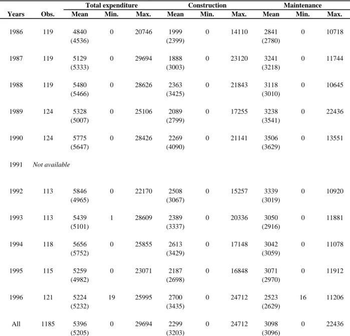
(15) loyalty e¤ect dominates.28 A dominant loyalty e¤ect would be consistent with the machine politics view of distributive politics, whereas a dominant political competition e¤ect would be consistent with the swing voter view. In sections 5 and 6, empirically-relevant versions of equation (8) will be estimated to test the theoretical model’s political competition e¤ect (governed by j. j). and loyalty e¤ect (governed by. ). Recall that according to the political competition e¤ect (see Proposition 1 above), one would. expect lower levels of expenditure where the intensity of political competition is low, e.g. where winning margins are typically high. The loyalty e¤ect concerns the role that local spending plays in securing the support of loyal districts in the future (see Proposition 2). According to the loyalty e¤ect, one would expect a positive relationship between expenditure and partisan loyalty.. 4. Data and Summary Statistics. To assess the empirical relevance of the political competition and the loyalty e¤ects described in the previous sections, I exploit rich data on the Québec government’s road expenditures in each of the province’s electoral districts. The expenditure data cover …scal years 1986 to 1996, with the exception of 1991, when the data were not compiled by the Department of Transportation.29 There were 122 (provincial) districts before 1989, and there has been 125 since then.30 The expenditure data set is merged with two other sources of data, used to construct district-level covariates. The …rst of these sources provides demographic and economic data on each electoral district. The second source of district-level data consists of o¢ cial election results covering six general elections (1981, 1985, 1989, 1994, 1998 and 2003). Summary statistics on the variables used in the analysis are provided in tables 1 and 2, which are now discussed in detail. 28. This case is a natural extension of the two-district model, in which such a positive correlation between. j. and. j. is implicitly assumed (see assumptions 1 and 2). 29 These …gures have been produced using administrative data, internal to the Department of Transportation – Béland (various years). Aggregate …gures may not match public accounts data. I refer to …scal years as if they were calendar years, e.g. 1986 refers to the 1986-87 …scal year. Publication of these data stopped after 1996. 30 Over the period covered by this study, some redistricting occurred but most changes to district boundaries have been minor. In these cases, it is straightforward to link old and new districts and no further adjustment to the data has been made. However, in some cases, either districts have been split or new districts have been created from existing districts. Thus, the number of cases varies from year to year. Another source of variation in the number of cases has to do with missing data points in the o¢ cial publications, which generally relate to urban districts where expenditure is very small.. 12.

(16) 4.1. Expenditure Data (Dependent Variable). Table 1 documents the road expenditure data, which are used to construct the dependent variable in all empirical speci…cations. The average per district road expenditure was $4.84 million in 1986 (in 1992 Canadian dollars) and reached a peak of $5.85 million in 1992.31 In 1996, average expenditure had declined to $5.22 million. The maximum spending received by a single district varied from $20.75 million (in 1986) to $29.69 million (in 1987). Each year, a fraction of the ‘ridings’–Canadian electoral districts – received zero or almost zero expenditure.32 The expenditure …gures include direct expenditure by the Department of Transportation on the construction and maintenance of roads under its direct jurisdiction and transfers to municipal governments for road improvement.33 On average, construction expenditure represents 42% of total expenditure (with a low of 37% in 1987 and a high of 52% in 1995), the remainder being accounted for by maintenance expenditure.. 4.2. District Characteristics. The following district characteristics are used in the analysis (see Table 2): the area covered by the district (AREAj ), the size of the population (P OPtj ), the share of the population living in urban areas (U RB j ), the share of the population that is French-speaking (F REN CHtj ), the number of manufacturing …rms (F IRM S j ), the unemployment rate (U Etj ), and the average household income (IN Ctj ).34 The AREAj variable is the only one to which a log transformation is applied in order to account for the wide size discrepancy between some large northern districts and the average district. This transformation conveniently linearizes the relationship between expenditure and district geographic size. Perhaps with the exception of population size, the districts vary widely with respect to these characteristics. Whereas the smallest district was 3 km2 (an urban district), the largest was 343,390 km2 (a northern district). The average riding had a population 31. All expenditure and income …gures are expressed in 1992 Canadian dollars using provincial CPI (data provided. by the Institut de la statistique du Québec). 32 A closer look at the data reveals that, each year, roughly one fourth of the ridings receives essentially no spending. These ridings are typically the smallest urban districts. 33 Most roads in Canada are under provincial/municipal jurisdiction. Any direct federal spending on infrastructure is not included here. 34 Data on district characteristics come from the Directeur général des élections du Québec, the body responsible for organizing elections in the province –see Directeur général des élections du Québec (various years). Most of these data come from special tabulations from the census and, hence, do not vary every year (see Table 1b for available years). Based on data availability, some of these variables are coded as time-invariant (they are AREAj ; U RB j and F IRM S j ).. 13.

(17) of 52,242 in 1986, 55,237 in 1991 and 57,099 in 1996. The share of the population living in urban areas varies from 10% to 100% and the share of the population whose main language is French (a group which forms more than 80% of the province’s population) ranges between 13% to 99%. The unemployment rate varies between 5.3% and 48.9%, while the average household’s real income is $24,813 in the ‘poorest’riding (in 1995) and $70,520 in the ‘richest’(in 1985).. 4.3. Election Data. Provincial politics in Québec, which is the focus of this paper, operates in a …rst-past-the-post system and was essentially bipartisan over the period of interest: the ‘federalist’ Québec Liberal Party and the ‘independentist’ Parti Québécois (PQ) have alternated in power since 1970.35 For the period most directly related to the expenditure data (1986-1996), the Liberals were in power from 1985 to 1994, when the PQ took o¢ ce, only to be replaced in power by the Liberals again in 2003. Table 3 provides some summary statistics on the elections held over the 1981-2003 period. From the electoral data, several political variables are constructed. The main political variables measure the intensity of political competition – not of long-run partisan loyalty – elections at the riding level. j. j. in the theoretical model – and the presence or. in the theoretical model. A standard measure of ‘closeness’of. (M ARtj ). is used as a proxy for the intensity of political competition.. This variable is de…ned in a straightforward manner for a particular district j and the last election before year t as36 vj1t M ARtj = PK. vj2t. k=1 vjkt. ;. (9). where vjkt is the number of votes cast for candidate k: K is the total number of candidates, and the candidates are ordered in decreasing order of their number of votes, such that vj1t stands for the number of votes for the winning candidate in district j, vj2t stands for the number of votes for the second most popular candidate, etc. Thus M ARtj captures the margin of the winner over total votes cast and will be used in the empirical analysis to capture the e¤ect of political competition. Summary statistics are provided in Table 2. There is wide variation in winning margins across districts. For example, in the 1985 election, winning margins ranged from .23% to 86.93%. The 35. Two other parties have been represented in the National Assembly (N.A.) over the 1981-2003 period: the ‘English-. speaking’Equality Party (four members of the N.A. in 1989) and the ‘conservative’Action démocratique du Québec (one elected in 1994). Separate elections are also held at the federal, municipal and school-board levels. 36 In election years, the previous election is also used. The same convention is adopted by Milligan and Smart (2005), who use a similar measure of election closeness.. 14.

(18) average margin was 20.47% in the 1985 election, 15.81% in the 1989 election, and 21.57% in the 1994 election. To capture a district’s loyalty to the party in power, six closely related measures of partisan loyalty are used. They exploit the fact that loyal districts repeatedly vote for a given party, often over long periods. All share the same logic: LOY ALjt = 1 if riding j repeatedly voted for the incumbent government in a given series of elections, 0 otherwise. The six loyalty variables (labeled L1 to L6) capture di¤erent combinations of elections (see Table 2 for details). For example, according to L1 a district is classi…ed as ‘loyal to the party in power’in year t if it voted for the party currently in power in the 1985, 1989 and 1994 elections.37 Depending on the measure being used, on average between 20% and 35% of districts can be classi…ed as ‘loyal’to the party in power. This approach to the measurement of partisan loyalty di¤ers from the approaches followed in Case (2001) and Larcinese, Rizzo and Testa (2006). In those studies, vote shares for the incumbent party are used as measures of what Larcinese et al. label ‘ideological bias.’38 To capture the dynamic aspect of partisan loyalty, the current application focuses on a measure of loyalty based on the extent of repeated support for the party in power. Finally, two variables describe the status of individual politicians in the Québec parliament (the National Assembly). The GOVtj variable takes values 1 if the district is represented by a member of the National Assembly (MNA) from the government party and 0 otherwise. In all three elections directly relevant to the expenditure data (1985, 1989 and 1994), majority governments were elected. Consequently, more than 50% of seats in the National Assembly were held by the government party, and as many as 82% following the 1985 election. Within the parliamentary delegation of the party in power, some MNAs are also cabinet members. The M INtj variable equals one if a district’s MNA was a cabinet minister during the previous calendar year, 0 otherwise. On average, one out of …ve MNAs were cabinet ministers in a given year between 1986 and 1996.. 5. Main Empirical Results. In this section, I study the relative roles played by political competition and partisan loyalty in the geographic allocation of road spending in Québec. The section proceeds as follows: Section 5.1 focuses on the e¤ect of political competition. The standard test of the political competition e¤ect in 37 38. In an election year, the party forming the incumbent government is deemed the party in power. In a related paper, Larcinese, Snyder and Testa (2006) measure ideological bias using exit polls. Such data are. not available in Québec.. 15.

(19) the literature involves regressing expenditure on a measure of election closeness, generally winning margin. As a benchmark, results based on this standard approach, i.e. abstracting from partisan loyalty, are presented. Measures of partisan loyalty are introduced in Section 5.2. Section 5.3 then explores the composition of road expenditure by presenting separate results for construction and maintenance expenditure.. 5.1. Political Competition. In this subsection, the basic estimating equation relates spending in district j and year t (EXPtj ) – the empirical counterpart of ej in the theoretical model – to winning margin (M ARtj ) in the previous election, controlling for a series of district characteristics: EXPtj = where. +. j G M ARt. GOVtj +. j O M ARt. OP Ptj + Zjt + Xj + 't +. is a constant, OP Ptj = 1 GOVtj , 't is a vector of year e¤ects, and. j. j. +. j t;. (10). is a vector of district. …xed e¤ects. The dependent variable is measured as the level of road spending.39 Zjt includes the political variables GOVtj and M INtj , and Xjt includes the following district characteristics: area covered by the district (AREAj ), population size (P OPtj ), urban population share (U RB j ), number of manufacturing …rms (F IRM S j ), unemployment rate (U Etj ) and household income (IN Ctj ). Note that this initial speci…cation excludes partisan loyalty, which will be introduced in Section 5.2, in order to focus …rst on the correlation between winning margin and expenditure. Equation (10) allows the e¤ect of winning margin on expenditure to di¤er between ridings held by the government (captured by the parameter 5.1.1. G). and opposition parties (. 40 O ).. Benchmark Results. The results for this benchmark regression are presented in the …rst two columns of Table 4.41 Speci…cation (1) includes the Xjt vector but no district …xed e¤ects.42 Most ‘economic’ controls enter the regression signi…cantly and with the expected signs. The area and urban population 39. Results are generally insensitive to changes in the de…nition of the dependent variable. Regressions using as the. dependent variable per capita expenditure, budget shares and ratios to the average district yield very similar results, and are available upon request. 40 Table 5 will also report benchmark results without this interaction – see Section 5.2. 41 Throughout the paper, standard errors are adjusted for clustering. Groups are de…ned according to the margin variable, which changes only once per electoral cycle in each district. 42 Since some district characteristics are coded as time-invariant, inclusion of …xed e¤ects absorbs them. In speci…cations (2) to (5), AREAj ; U RB j and F IRM S j are dropped and …xed e¤ects are included.. 16.

(20) variables are strongly signi…cant, with a positive sign for the former and a negative sign for the latter. The unemployment rate is also signi…cant and enters the regression positively (higher unemployment being associated with more spending), perhaps re‡ecting the role of transportation infrastructure in regional development policies. While the positive signs on the other two economic variables (income and number of …rms) suggest a positive relationship between economic activity and spending, only the number of …rms coe¢ cient is statistically signi…cant.43 Turning now to the political variables, the main parameters of interest are tively the coe¢ cients on. M ARtj. GOVtj. and. M ARtj. OP Ptj ):. G. and. O. (respec-. The basic empirical test can be. thought of as follows: consistent with the swing voter view of distributive politics, the theoretical model’s political competition e¤ect predicts that both. G. and. O. should be negative. Accord-. ing to this e¤ect, more spending should be directed to ridings with narrow margins regardless of which party currently holds the riding, those ridings being the most likely to be pivotal in the next election.44 However, Speci…cation (1) displays a strong positive e¤ect of winning margin in government-held ridings (^G > 0). This result thus seems to sharply contradict the swing voter view of distributive politics and is more in line with the machine politics view. The coe¢ cient on M ARtj. OP Ptj has the expected negative sign but is not statistically signi…cant. The other two. political variables (GOVtj and M INtj ) display insigni…cant e¤ects. Speci…cation (2) exploits the panel structure of the data. By including …xed e¤ects, it controls for …xed unchanging district characteristics. The results for Speci…cation (2) show that ^G and ^O have the same signs as in Speci…cation (1) but neither of them is statistically signi…cant, with ^G now much smaller. Again, these results provide very little evidence in favour of the swing voter view. Speci…cation (3) presents the results from a …xed-e¤ects regression on the subsample of districts that were in the …rst three deciles of the winning margin variable in 1985. The results from this speci…cation provide useful information with respect to a potentially nonlinear e¤ect of the winning margin on expenditure. Indeed, it is for the highest margins that one would expect the swing district prediction to be the weakest. Hence, limiting the sample to close races introduces a bias against …nding machine politics patterns, which are intuitively expected to be more prevalent for 43. The number of manufacturing …rms is central to the analysis of Cadot et al. (2006), which they interpret as a. proxy for lobbying activities. My results corroborate the presence of a signi…cant link between the number of …rms and spending. 44 As shown by Lemma 1’ in Appendix A.3, there is no a priori reason to expect that the political competition e¤ect should work di¤erently in government and opposition districts.. 17.

(21) higher margins. Both ^G and ^O now have the negative sign predicted by the political competition e¤ect. While the e¤ect is now signi…cant for opposition-held ridings, it is still insigni…cant for government-held ridings.45 5.1.2. Electoral Budget Cycle. The …rst three speci…cations in Table 4 make the strong assumption that the impact of political variables such as M ARtj GOVtj are constant over time. Speci…cations (4) and (5) allow the impact of M ARtj GOVtj to vary over the electoral cycle.46 In Speci…cation (4), M ARtj GOVtj is interacted with three electoral cycle dummies: ELECt (election years: 1989 and 1994), P REELECt (preelection years: 1988 and 1993), and P OST ELECt (post-election years: 1986, 1990 and 1995). The coe¢ cients on all three interaction terms are positive. However, M ARtj. GOVtj is only signi…cant. when interacted with the ELECt dummy, revealing that a lot of the action is concentrated in election years. Note that the coe¢ cient on M ARtj. OP Ptj (which is not interacted with electoral. cycle dummies here) has the expected negative sign and is marginally signi…cant. Speci…cation (5) is presented as a robustness test for the positive sign on M ARtj. GOVtj. ELECt in Speci…cation. (4). Interactions with P REELECt and P OST ELECt are dropped, and year e¤ects are included. The pattern of interest (the positive sign on the estimated coe¢ cient for M ARtj GOVtj ELECt ) appears to be robust. These results indicate that the dynamics in opposition ridings tend to conform to the standard swing voter view but that, in government-held ridings, there is no supporting evidence.47 Furthermore, the e¤ect of winning margin is positive and signi…cant in election years, when electoral 45. It may be argued that Speci…cation (3) controls for the potential endogeneity of political variables, at least to. some degree. According to Lee et al. (2004), by following over time a subgroup of districts where winning margins were initially narrow, it is possible to isolate a group of districts that share similar unobservable characteristics. Unfortunately, given that the variable of interest here is the winning margin, this strategy is obviously not fully satisfactory for our purposes since using margin to split the sample e¤ectively treats it as a control variable. Note also that there is a trade-o¤ here in restricting the sample to closer races, which would arguably reduce the endogeneity bias but also reduce the number of observations and hence the precision of the results. Unreported results show that choosing a lower cuto¤ does not signi…cantly alter the qualitative pattern of the political variables. For a more comprehensive discussion of potential endogeneity issues, see Section 6. 46 There is a large body of literature on political budget cycles, the well-known phenomenon that aggregate government budget ‡uctuations are in‡uenced by political dynamics. Brender and Drazen (2005) revisit the evidence on the political budget cycle and, in a related paper, Drazen and Eslava (2006) provide a theoretical model of redistributive politics in which swing regions are targeted before the election. 47 Milligan and Smart (2005) …nd a similar dichotomy.. 18.

(22) competition is expected to be the strongest. On average, government-held ridings with high winning margins in the previous election received higher road spending in election years. The estimated e¤ect is economically signi…cant, a one percentage-point increase in winning margin being associated with $40,000 worth of spending in election years. The remainder of this section argues that this pattern is largely explained by the positive correlation between winning margin and partisan loyalty.. 5.2. Partisan Loyalty. The large positive coe¢ cients on M ARtj estimated for government-held ridings in the previous subsection are puzzling if one’s prior is the swing voter view of distributive politics. Why would rational politicians not target swing districts, especially close to an election? I argue that these estimates might su¤er from an omitted variable bias related to the role played by partisan loyalty. High margins tend to be associated with strong partisan loyalty. And the theoretical model of Section 2 develops one rationale as to why loyalty might be a determinant of the allocation of spending across districts. In terms of equation (10), the coe¢ cient on M ARtj GOVtj will be biased if (i) M ARtj GOVtj is correlated with partisan loyalty, and (ii) if the error term. j t. is also correlated. with loyalty. Regardless of the loyalty measure (L1 to L6) being used, there is indeed a strong positive correlation between M ARtj and LOY ALjt (see the last column of Table 5). The coe¢ cient of correlation between these two variables varies from .28 for L4 (loyalty de…ned over all future elections) to .50 for L3 (loyalty de…ned over all past elections) and is always signi…cantly di¤erent from zero at the 1% con…dence level. Omitting loyalty from the regressions will therefore be a concern to the extent that partisan loyalty is in itself a factor in the geographic allocation of spending, as suggested by the theoretical model. In this subsection, I take this concern seriously and present results based on the following equation: EXPtj =. + M ARtj + LOY ALjt + Zjt + Xjt + 't +. j. +. j t:. (11). This speci…cation includes the partisan loyalty variable and provides evidence on the relative in‡uence of political competition and loyalty on the allocation of spending. The main parameters of interest are now. and : In line with the swing voter view, ^ is expected to be negative. Consistent with the machine politics view, ^ is expected to be positive.48 48. Since the focus of this subsection is on the partisan loyalty e¤ect, the regressions do not allow the e¤ect of winning. 19.

(23) Table 5 reports results from regressions with the six loyalty variables, with and without …xed e¤ects. It also reports the results from a benchmark regression excluding LOY ALjt . Mirroring the results presented above, the coe¢ cient on M ARtj (^ ) is positive and signi…cant in the benchmark regression. Regardless of which loyalty measure is being used, the inclusion of LOY ALjt in the regression considerably decreases the coe¢ cient on M ARtj : Although it remains positive in most cases, it is never signi…cant. In contrast, the coe¢ cient on LOY ALj (^) is positive and signi…cant t. at the 1% con…dence level in all speci…cations but one. When equation (11) is estimated with …xed e¤ects, the coe¢ cient on LOY ALjt is still positive but not signi…cant.49 The sudden explanatory power of the GOVtj variable when …xed e¤ects and the loyalty variable are introduced is puzzling, as it is the only speci…cation in which this variable displays a signi…cant e¤ect. Note that with …xed e¤ects, the impact of loyalty – essentially a …xed district characteristic – is identi…ed from changes in the loyalty variable. By construction of the loyalty variables used in this study, such changes occur only when there is a change in government. In the current context, this occurred only in 1994. Given this limited variation, changes in the loyalty variable are hard to disentangle from changes in the GOVtj variable, many of which correspond to the changes in LOY ALjt – see Section 6.2 for a di¤erence-in-di¤erences strategy which actually exploits the 1994 change in government. To address this concern, I also provide results from a …xed-e¤ect regression without the GOVtj variable. These results show an estimate of the e¤ect of loyalty that is strongly signi…cant. Although smaller in magnitude than in the regressions without …xed e¤ects, the latter e¤ect is economically signi…cant: it implies that a loyal district received 17% more spending than the average district.. 5.3. Construction vs. Maintenance Expenditure. The data allow for a separate analysis of construction and maintenance expenditure, with the former containing major road improvement projects. One might expect maintenance expenditure to be less responsive to political considerations and more responsive to local needs than construction expenditure. This is indeed what the results in the last two lines of Table 5 indicate. While partisan loyalty has a positive and strongly signi…cant e¤ect on construction expenditure, the e¤ect margin to di¤er in government-held and opposition-held districts. However, note that since loyalty to the party in power is taken into account, one should not expect a di¤erence in the e¤ect of winning margin in government vs. opposition ridings – see Appendix A.3. 49 Table 5 presents results for …xed e¤ects regressions only with loyalty measure L2. As shown by results for the six loyalty measures without …xed e¤ects, the results are only slightly sensitive to the de…nition of LOY ALjt :. 20.

(24) is considerably smaller (and not signi…cant) for maintenance expenditure. This result suggests that major projects, presumably those with the biggest long-term value to voters, are being driven by partisan loyalty. The positive coe¢ cient on M ARtj in the maintenance expenditure regression (signi…cant at the 10% level) is hard to interpret and once again casts doubt on the presence of a signi…cant political competition e¤ect in the behaviour of Québec governments over the 1986-1996 period. Taken together, the results presented in this section illustrate the di¢ culty of identifying any evidence of the standard swing voter view in the Québec data. They do, however, provide stronger support for the machine politics view. Section 6 below shows that this overall picture is robust when accounting for the potential endogeneity of political variables.. 6. Robustness and Endogeneity. In this section, the robustness of the results presented in Section 5 is assessed by means of instrumental variables (IV) and di¤erence-in-di¤erences strategies to account for the potential endogeneity of the LOY ALjt variable. As suggested by the theory discussion in Section 2, partisan loyalty is the product of repeated interaction between parties and voters. Hence, while loyalty can be expected to be a causal factor in the allocation of spending, it is also likely that causality works in the opposite direction if governments actually spend with the intention to nurture local partisan loyalties. More generally, endogeneity biases will arise if non-observable considerations, e.g. preferences for public goods, are correlated with both electoral outcomes (speci…cally partisan loyalty) and the geographic allocation of road spending. To get a sense of the likelihood that partisan loyalty is picking up some unobserved heterogeneity across districts, Table 7 compares the 28 districts that were loyal to the Liberal party in all elections between 1981 and 2003 (i.e. according to L2) to the other 97 districts, based on observable characteristics. Suggesting that unobserved heterogeneity might be an issue, ‘Liberal strongholds’are statistically di¤erent from the other districts along three dimensions: loyal districts tend to be slightly smaller, have a lower unemployment rate, and have a much smaller share of French-speakers. The latter is the main observable di¤erence between liberal strongholds and other districts and will form the basis for the IV strategy that follows. Based on these observations, the direction of the potential OLS bias a¤ecting the LOY ALjt coe¢ cient is unclear. On the one hand, Liberal strongholds tend to be economically dynamic areas. 21.

(25) (as suggested by the low unemployment rate) and hence can be expected to have a strong need for new or improved roads. If this is true, one should expect the OLS estimates to be upward-biased. On the other hand, Liberal strongholds tend to be small urban districts, which can be expected to be characterized by a low preference for road spending compared to other public spending. This alternative story suggests that OLS estimates might instead be downward-biased.. 6.1. Instrumental Variables. The IV strategy uses the French-speaking population variable (F REN CHtj ) as an instrument for partisan loyalty. The rationale for this instrument comes from a fundamental characteristic of the political environment in Québec: partisan loyalties and language spoken are strongly correlated. Roughly 80% of the province’s 7-million population are French-speaking, the majority of whom descend from original French settlers and have a Roman Catholic background. The English-speaking population, which forms a majority in Canada as a whole, is the most important linguistic minority in Québec. This British (and usually Protestant) presence in Québec goes as far back as 1760, when New France was integrated in the British Empire. The Parti Québécois, which advocates the province’s independence from Canada, draws almost all of its support from the French-speaking community. In contrast, loyalty to the Liberal Party (in o¢ ce for most of the period covered by this study) tends to arise in districts where the English-speaking population is concentrated (e.g. Western Montréal). Anecdotal evidence for this is provided by the fact that among the 12 strongest wins for the Liberals in 1985 (the top decile), 11 occurred in Western Montréal ridings. The IV regressions are conducted under the assumption that language is in itself not a direct determinant of the level of transportation expenditure received by a district. If language has an in‡uence on spending patterns, it is taken here to be mediated by the political process (through its in‡uence on partisan loyalty). This is what the …rst stage regression captures: the linguistic composition of a riding is a key determinant of the nature of partisan loyalty in that riding. In the second stage, partisan loyalty itself (together with the intensity of political competition) captures the ability of politicians to bias the allocation of spending for electoral purposes. The bottom panel of Table 6 presents …rst-stage diagnostics documenting the strong correlation between F REN CHtj and LOY ALjt : The correlation between the two variables is strong, ranging from .29 for loyalty variable L1 to .46 for L5. The usual F -tests and partial R2 measures con…rm that, regardless of which de…nition of the loyalty variable is used, F REN CHtj has strong predictive power in the …rst-stage regression.. 22.

(26) IV results, featured in the top panel of Table 6, are qualitatively similar to the previous results. In fact, the e¤ect of partisan loyalty is slightly bigger and still statistically signi…cant in all speci…cations (except again for maintenance expenditure). The coe¢ cient on winning margin is negative in most speci…cations but, as before, is never signi…cantly di¤erent from zero. These results con…rm the robustness of the previous section’s results, and suggest that causality is working in the expected direction, i.e. from partisan loyalty to spending. The fact that the IV estimates tend to be bigger than their OLS counterparts is noteworthy and likely due to the fact that the …rst-stage regression underscores the e¤ect of politically powerful English-speaking ridings (the core supporters of the Liberal party), hence reinforcing the estimated impact of loyalty on expenditure. As suggested by Dixit and Londregan (1996), it may be less expensive for the government to cater to its core supporters, for organizational or informational reasons. If this is the case, then IV results will remain upward biased. Nevertheless, even if they do not allow for a direct test of the theoretical model of Section 2 against Dixit and Londregan’s model, these IV results suggest that core supporters within loyal districts are driving the spending allocation in their favour. Indeed, the F REN CHtj variable can be interpreted as a rough proxy for the within-district distribution of partisan loyalties in Québec. And results show that a large proportion, in a district, of the language group that is traditionally loyal to the party in power tends to reinforce the correlation between a district’s loyalty and road spending.. 6.2. Di¤erence-in-Di¤erences. An additional caveat of the above IV strategy follows from the fact that F REN CHtj is essentially a time-invariant district characteristic. Therefore, in this particular application, it is not a suitable instrument in the …xed e¤ects regressions (…xed e¤ects are accordingly excluded from the IV regression). But the fact that there was a change of government in 1994 allows for a di¤erent identi…cation strategy which exploits variation over time in the loyalty variable. The rationale is simple: the extra spending directed to ridings that are loyal to the Liberals while this party is in power should go away when the PQ takes o¢ ce in 1994. This suggests a di¤erence-in-di¤erences strategy that compares spending in ridings that are loyal to the Liberals (l) to spending in the other ridings (o), before and after the 1994 election. Here, the e¤ect of partisan loyalty is identi…ed as follows: ^ = (EXP l. 86 94. l. EXP 95. 96 ). o. (EXP 86. o. 94. EXP 95. 96 ). (12). where the upper bars denote averages. In terms of controlling for the potential endogeneity of 23.

(27) partisan loyalty, the main advantage of this approach is that it di¤erences out any …xed systematic di¤erence between ridings that are loyal to the Liberal party and the rest of the province. Figure 1 provides visual evidence corresponding to this identi…cation strategy. Ridings that can be classi…ed as loyal to the Liberals clearly bene…ted from an advantage in terms of road construction expenditure when that party was in power (between 1985 and 1994). Although that advantage varied from year to year during the two Liberal mandates, it was present in every year for which data are available (remember that the data were not collected in 1991). It was especially large around the 1989 election and again in 1993, a pre-election year. Following the 1994 election, in which the PQ returned to power, Liberal strongholds experienced a sudden drop in road expenditure. Meanwhile, the other ridings (which include those loyal to the PQ) saw their spending level rise importantly in 1996. As a result, in the two years after the 1994 election for which expenditure is available, Liberal strongholds received less construction spending than the other ridings.. Figure 1: Road construction expenditure in Liberal strongholds vs. other ridings. Table 8 presents the results pertaining to this di¤erence-in-di¤erences exercise. Results are presented for all expenditure and for construction and maintenance expenditure separately. I also. 24.