CIRPÉE
Centre interuniversitaire sur le risque, les politiques économiques et l’emploi
Cahier de recherche/Working Paper 06-09
Testing for Restricted Stochastic Dominance
Russell Davidson Jean-Yves Duclos
Mars/March 2006
_______________________
Davidson: Department of Economics and CIREQ, McGill University, Montréal, Québec, Canada H3A 2T7; GREQAM, Centre de la Vieille Charité, 2 Rue de la Charité, 13236 Marseille cedex 02, France
Duclos: Department of Economics and CIRPÉE, Université Laval, Ste-Foy, Québec, Canada G1K 7P4
This research was supported by the Canada Research Chair program (Chair in Economics, McGill University) and by grants from the Social Sciences and Humanities Research Council of Canada, the Fonds Québécois de Recherche sur la Société et la Culture, and the PEP Network of the International Development Research Centre.
Abstract:
Asymptotic and bootstrap tests are studied for testing whether there is a relation of stochastic dominance between two distributions. These tests have a null hypothesis of nondominance, with the advantage that, if this null is rejected, then all that is left is dominance. This also leads us to define and focus on restricted stochastic dominance, the only empirically useful form of dominance relation that we can seek to infer in many settings. One testing procedure that we consider is based on an empirical likelihood ratio. The computations necessary for obtaining a test statistic also provide estimates of the distributions under study that satisfy the null hypothesis, on the frontier between dominance and nondominance. These estimates can be used to perform bootstrap tests that can turn out to provide much improved reliability of inference compared with the asymptotic tests so far proposed in the literature.
Keywords: Stochastic dominance, empirical likelihood, bootstrap test JEL Classification: C100, C120, C150, I320
1. Introduction
Consider two probability distributions, A and B, characterised by cumulative
distri-bution functions (CDFs) FA and FB. In practical applications, these distributions
might be distributions of income, before or after tax, wealth, or of returns on financial assets. Distribution B is said to dominate distribution A stochastically at first order
if, for all z in the union of the supports of the two distributions, FA(z) ≥ FB(z). If B
dominates A, then it is well known that expected utility and social welfare are greater in B than in A for all utility and social welfare functions that are symmetric and monotonically increasing in returns or in incomes, and that all poverty indices that are symmetric and monotonically decreasing in incomes are smaller in B than in A.
These are powerful orderings of the two distributions1 and it is therefore not surprising
that a considerable empirical literature has sought to test for stochastic dominance at first and higher orders in recent decades.
Testing for dominance, however, requires leaping over a number of hurdles. First, there is the possibility that population dominance curves may cross, while the sample ones do not. Second, the sample curves may be too close to allow a reliable ranking of the population curves. Third, there may be too little sample information from the tails of the distributions to be able to distinguish dominance curves statistically over their entire theoretical domain. Fourth, testing for dominance typically involves distinguishing curves over an interval of an infinity of points, and therefore should also involve testing differences in curves over an infinity of points. Fifth, the overall testing procedure should take into account the dependence of a large number of tests carried out jointly over an interval. Finally, dominance tests are always performed with finite samples, and this may give rise to concerns when the properties of the procedures that are used are known only asymptotically.
Until now, the most common way to test whether there is stochastic dominance, on the basis of samples drawn from the two populations A and B, is to posit a null hypothesis of dominance, and then to study test statistics that may or may not lead to rejection of
this hypothesis2. Rejection of a null of dominance is, however, an inconclusive outcome
in the sense that it fails to rank the two populations. In the absence of information on the power of the tests, non-rejection of dominance does not enable one to accept dominance, the usual outcome of interest. It may thus be preferable, from a logical point of view, to posit a null of nondominance, since, if we succeed in rejecting this null, we may legitimately infer the only other possibility, namely dominance.
We adopt this latter standpoint in this paper. We find that it leads to testing proce-dures that are actually simpler to implement than conventional proceproce-dures in which
1 See Levy (1992) for a review of the breadth of these orderings, and Hadar and Russell
(1969) andHanoch and Levy (1969) for early developments.
2 See, for instance, Beach and Richmond (1985), McFadden (1989), Klecan, McFadden
and McFadden (1991),Bishop, Formby and Thistle (1992), Anderson (1996), Davidson and Duclos (2000), Barrett and Donald (2003), Linton, Maasoumi and Whang (2005), andMaasoumi and Heshmati (2005).
the null is dominance. The simplest procedure for testing nondominance was proposed
originally by Kaur, Prakasa Rao, and Singh (1994) (henceforth KPS) for continuous
distributions A and B, and a similar test was proposed in an unpublished paper by Howes (1993a)for discrete distributions. In this paper, we develop an alternative pro-cedure, based on an empirical likelihood ratio statistic. It turns out that this statistic is always numerically very similar to the KPS statistic in all the cases we consider. However, the empirical likelihood approach produces as a by-product a set of proba-bilities that can be interpreted as estimates of the population probaproba-bilities under the assumption of nondominance.
These probabilities make it possible to set up a bootstrap data-generating process (DGP) which lies on the frontier of the null hypothesis of nondominance. We show that, on this frontier, both the KPS and the empirical likelihood statistics are asymptotically pivotal, by which we mean that they have the same asymptotic distribution for all configurations of the population distributions that lie on the frontier. A major finding of this paper is that bootstrap tests that make use of the bootstrap DGP we define can yield much more satisfactory inference than tests based on the asymptotic distributions of the statistics.
The paper also shows that it is not possible with continuous distributions to reject nondominance in favour of dominance over the entire supports of the distributions. Accepting dominance is empirically sensible only over restricted ranges of incomes or returns. This necessitates a recasting of the usual theoretical links between stochastic dominance relationships and orderings in terms of poverty, social welfare and expected utility. It also highlights better why a non-rejection of the usual null hypothesis of unrestricted dominance cannot be interpreted as an acceptance of dominance, since unrestricted dominance can never be inferred from continuous data.
In Section 2, we investigate the use of empirical likelihood methods for estimation of distributions under the constraint that they lie on the frontier of nondominance, and develop the empirical likelihood ratio statistic. The statistic is a minimum over all the points of the realised samples of an empirical likelihood ratio that can be defined
for all points z in the support of the two distributions. In Section 3 we recall the
KPS statistic, which is defined as a minimum over z of a t statistic, and show that
the two statistics are locally equivalent for all z at which FA(z) = FB(z). Section 4
shows why it turns out to be impossible to reject the null of nondominance when the population distributions are continuous in their tails. Some connections between this
statistical fact and ethical considerations are explored in Section 5, and the concept
of restricted stochastic dominance is introduced. In Section 6, we discuss how to test
restricted stochastic dominance, and then, inSection 7we develop procedures for
test-ing the null of nondominance, in which we are obliged to censor the distributions, not necessarily everywhere, but at least in the tails. In that section, we also show that, for configurations of nondominance that are not on the frontier, the rejection probabilities of tests based on either of our two statistics are no greater than they are
cance level, then the probability of Type I error in the interior of the null hypothesis is no greater than that on the frontier. We are then able to show that the statistics are
asymptotically pivotal on the frontier. Section 8 presents the results of a set of Monte
Carlo experiments in which we investigate the rejection probabilities of both asymp-totic and bootstrap tests, under the null and under some alternative setups in which there actually is dominance. We find that bootstrapping can lead to very considerable
gains in the reliability of inference. Section 9 illustrates the use of the techniques with
data drawn from the Luxembourg Income Study surveys, and finds that, even with relatively large sample sizes, asymptotic and bootstrap procedures can lead to different
inferences. Conclusions and some related discussion are presented in Section 10.
2. Stochastic Dominance and Empirical Likelihood
Let two distributions, A and B, be characterised by their cumulative distribution
functions (CDFs) FA and FB. Distribution B stochastically dominates A at first order
if, for all x in the union U of the supports of the two distributions, FA(x) ≥ FB(x). In
much theoretical writing, this definition also includes the condition that there should
exist at least one x for which FA(x) > FB(x) strictly. Since in this paper we are
concerned with statistical issues, we ignore this distinction between weak and strong dominance since no statistical test can possibly distinguish between them.
Suppose now that we have two samples, one each drawn from the distributions A
and B. We assume for simplicity that the two samples are independent. Let NA
and NB denote the sizes of the samples drawn from distributions A and B respectively.
Let YA and YB denote respectively the sets of (distinct) realisations in samples A
and B, and let Y be the union of YA and YB. If, for K = A, B, yK
t is a point in YK,
let the positive integer nK
t be the number of realisations in sample K equal to ytK.
This setup is general enough for us to be able to handle continuous distributions, for
which all the nK
t = 1 with probability 1, and discrete distributions, for which this is
not the case. In particular, discrete distributions may arise from a discretisation of continuous distributions. The empirical distribution functions (EDFs) of the samples can then be defined as follows. For any z ∈ U , we have
ˆ FK(z) = 1 NK NK X t=1 I(yKt ≤ z),
where I(·) is an indicator function, with value 1 if the condition is true, and 0 if not.
If it is the case that ˆFA(y) ≥ ˆFB(y) for all y ∈ Y , we say that we have first-order
stochastic dominance of A by B in the sample.
In order to conclude that B dominates A with a given degree of confidence, we require that we can reject the null hypothesis of nondominance of A by B with that degree of confidence. Such a rejection may be given by a variety of tests. In this section we develop an empirical likelihood ratio statistic on which a test of the null of
As should become clear, it is relatively straightforward to generalise the approach to second and higher orders of dominance, although solutions such as those obtained analytically here would then need to be obtained numerically.
For a given sample, the “parameters” of the empirical likelihood are the probabilities associated with each point in the sample. The empirical loglikelihood function (ELF)
is then the sum of the logarithms of these probabilities. If as above we denote by nt
the multiplicity of a realisation yt, the ELF is
P
yt∈Y ntlog pt, where Y is the set of
all realisations, and the pt are the “parameters”. If there are no constraints, the ELF
is maximised by solving the problem max pt X yt∈Y ntlog pt subject to X yt∈Y pt = 1.
It is easy to see that the solution to this problem is pt = nt/N for all t, N being the
sample size, and that the maximised ELF is −N log N +Ptntlog nt, an expression
which has a well-known entropy interpretation.
With two samples, A and B, using the notation given above, we see that the proba-bilities that solve the problem of the unconstrained maximisation of the total ELF are pK
t = nKt /NK for K = A, B, and that the maximised ELF is
−NAlog NA− NBlog NB+ X yA t ∈YA nAt log nAt + X yB t ∈YB nBt log nBt . (1)
Notice that, in the continuous case, and in general whenever nK
t = 1, the term
nK
t log nKt vanishes.
The null hypothesis we wish to consider is that B does not dominate A, that is, that
there exists at least one z in the interior of U such that FA(z) ≤ FB(z). We need z to
be in the interior of U because, at the lower and upper limits of the joint support U, we
always have FA(z) = FB(z), since both are either 0 or 1. In the samples, we exclude
the smallest and greatest points in the set Y of realisations, for the same reason. We
write Y◦ for the set Y without its two extreme points. If there is a y ∈ Y◦ such that
ˆ
FA(y) ≤ ˆFB(y), there is nondominance in the samples, and, in such cases, we plainly
do not wish to reject the null of nondominance. This is clear in likelihood terms, since the unconstrained probability estimates satisfy the constraints of the null hypothesis, and so are also the constrained estimates.
If there is dominance in the samples, then the constrained estimates must be different from the unconstrained ones, and the empirical loglikelihood maximised under the constraints of the null is smaller than the unconstrained maximum value. In order to
satisfy the null, we need in general only one z in the interior of U such that FA(z) =
FB(z). Thus, in order to maximise the ELF under the constraint of the null, we begin
For given z, the constraint we wish to impose can be written as X yA t ∈YA pAt I(ytA≤ z) = X yB s∈YB pBsI(ysB ≤ z), (2)
where the I(·) are again indicator functions. If we denote by FK(pK; ·) the
cumu-lative distribution function with points of support the yK
t and corresponding
proba-bilities the pK
t , then it can be seen that condition (2) imposes the requirement that
FA(pA, z) = FB(pB, z).
The maximisation problem can be stated as follows: max pA t ,pBs X yA t ∈YA nAt log pAt + X yB s∈YB nBs log pBs subject to X yA t ∈YA pA t = 1, X yB s∈YB pB s = 1, X yA t ∈YA pA t I(ytA ≤ z) = X yB s∈YB pB sI(ysB ≤ z).
The Lagrangian for this constrained maximisation of the ELF is X t nAt log pAt +X s nBs log pBs + λA Ã 1 −X t pAt ! + λB Ã 1 −X s pBs ! −µ Ã X t pAt I(ytA≤ z) −X s pBsI(yBs ≤ z) ! ,
with obvious notation for sums over all points in YA and YB, and where we define
Lagrange multipliers λA, λB, and µ for the three constraints.
The first-order conditions are the constraints themselves and the relations
pAt = n A t λA+ µI(yAt ≤ z) and pBs = n B s λB− µI(ysB ≤ z) . (3) Since PtpA t = 1, we find that λA= X t λAnAt λA+ µIt(z) =X t nAt λA+ µIt(z) λA+ µIt(z) − µX t nA t It(z) λA+ µIt(z) = NA− µ λA+ µ X t nA t It(z) = NA− µ λA+ µ NA(z), (4)
where It(z) ≡ I(yAt ≤ z) and NA(z) =
P
tnAt It(z) is the number of points in sample A
less than or equal to z. Similarly,
λB = NB+
µ λB − µ
with NB(z) =
P
snBsIs(z). With the relations (3), the constraint (2) becomes
X t It(z) λA+ µ = X s Is(z) λB − µ, that is, NA(z) λA+ µ = NB(z) λB− µ. (6)
Thus, adding (4) and (5), we see that
λA+ λB = NA+ NB = N, (7)
where N ≡ NA+ NB.
If we make the definition ν ≡ λA+ µ, then, from (7), λB− µ = N − λA− µ = N − ν.
Thus (6) becomes
NA(z)
ν =
NB(z)
N − ν. (8)
Solving for ν, we obtain
ν = N NA(z)
NA(z) + NB(z). (9)
From (4), we see that
λA= NA− NA(z) + λANA(z) λA+ µ so that 1 = NA− NA(z) λA + NA(z) λA+ µ . (10) Similarly, from (5), 1 = NB − NB(z) λB + NB(z) λB− µ . (11)
Write λ ≡ λA, and define MK(z) = NK−NK(z). Then (10) and (11) combine with (6)
to give
MA(z)
λ =
MB(z)
N − λ. (12)
Solving for λ, we see that
λ = N MA(z)
MA(z) + MB(z). (13)
The probabilities (3) can now be written in terms of the data alone using (9) and (13). We find that pAt = n A t It(z) ν + nA t (1 − It(z)) λ and p B s = nB sIs(z) N − ν + nB s (1 − Is(z)) N − λ . (14)
We may use these in order to express the value of the ELF maximised under constraint as
X
Twice the difference between the unconstrained maximum (1), which can be written
as X
t
nAt log nAt +X
s
nBs log nBs − NAlog NA− NBlog NB,
and the constrained maximum (15) is an empirical likelihood ratio statistic. Using (9) and (13) for ν and λ, the statistic can be seen to satisfy the relation
1
−2LR(z) = N log N − NAlog NA− NBlog NB+ NA(z) log NA(z) + NB(z) log NB(z)
+MA(z) log MA(z) + MB(z) log MB(z) − ¡ NA(z) + NB(z) ¢ log¡NA(z) + NB(z) ¢ −¡MA(z) + MB(z) ¢ log¡MA(z) + MB(z) ¢ . (16)
We will see later how to use the statistic in order to test the hypothesis of nondomi-nance.
3. The Minimum t Statistic
In Kaur, Prakasa Rao, and Singh (1994), a test is proposed based on the minimum of
the t statistic for the hypothesis that FA(z) − FB(z) = 0, computed for each value of z
in some closed interval contained in the interior of U. The minimum value is used as the test statistic for the null of nondominance against the alternative of dominance. The test can be interpreted as an intersection-union test. It is shown that the probability of rejection of the null when it is true is asymptotically bounded by the nominal level
of a test based on the standard normal distribution. Howes (1993a) proposed a very
similar intersection-union test, except that the t statistics are calculated only for the predetermined grid of points.
In this section, we show that the empirical likelihood ratio statistic (16) developed in
the previous section, where the constraint is that FA(z) = FB(z) for some z in the
interior of U, is locally equivalent to the square of the t statistic with that constraint
as its null, under the assumption that indeed FA(z) = FB(z).
Since we have assumed that the two samples are independent, the variance of ˆFA(z) −
ˆ
FB(z) is just the sum of the variances of the two terms. The variance of ˆFK(z),
K = A, B, is FK(z)
¡
1 − FK(z)
¢
/NK, where NK is as usual the size of the sample from
population K, and this variance can be estimated by replacing FK(z) by ˆFK(z). Thus
the square of the t statistic is
t2(z) = NANB ¡ˆ FA(z) − ˆFB(z) ¢2 NBFˆA(z) ¡ 1 − ˆFA(z) ¢ + NAFˆB(z) ¡ 1 − ˆFB(z) ¢ . (17)
Suppose that FA(z) = FB(z) and denote their common value by F (z). Also define
∆(z) ≡ ˆFA(z) − ˆFB(z). For the purposes of asymptotic theory, we consider the limit
in which, as N → ∞, NA/N tends to a constant r, 0 < r < 1. It follows that
ˆ
The statistic (17) can therefore be expressed as the sum of its leading-order asymptotic term and a term that tends to 0 as N → ∞:
t2(z) = r(1 − r)
F (z)(1 − F (z))N →∞plim
N ∆2(z) + O
p(N−1/2). (18)
It can now be shown that the statistic LR(z) given by (16) is also equal to the right-hand side of (18) under the same assumptions as those that led to (18). The algebra is rather messy, and so we state the result as a theorem.
Theorem 1
As the size N of the combined sample tends to infinity in such a way that NA/N → r, 0 < r < 1, the statistic LR(z) defined by (16) tends to the
right-hand side of (18) for any point z in the interior of U, the union of the supports
of populations A and B, such that FA(z) = FB(z).
Proof: In Appendix. Remarks:
It is important to note that, for the result of the above theorem and for (18) to hold, the point z must be in the interior of U . As we will see in the next section, the behaviour of the statistics in the tails of the distributions is not adequately represented by the asymptotic analysis of this section.
It is clear that both of the two statistics are invariant under monotonically increasing transformations of the measurement units, in the sense that if an income z is
trans-formed into an income z0 in a new system of measurement, then t2(z) in the old system
is equal to t(z0) in the new, and similarly for LR(z) .
Corollary
Under local alternatives to the null hypothesis that FA(z) = FB(z), where
FA(z) − FB(z) is of order N−1/2 as N → ∞, the local equivalence of t2(z)
and LR(z) continues to hold. Proof:
Let FA(z) = F (z) and FB(z) = F (z) − N−1/2δ(z), where δ(z) is independent of N .
Then ∆(z) is still of order N−1/2 and the limiting expression on the right-hand side
of (18) is unchanged. The common asymptotic distribution of the two statistics now has a positive noncentrality parameter.
4. The Tails of the Distribution
Although the null of nondominance has the attractive property that, if it is rejected, all that is left is dominance, this property comes at a cost, which is that it is impossible to infer dominance over the full support of the distributions if these distributions are continuous in the tails. This reinforces our earlier warning that non-rejection of the literature’s earlier null hypotheses of dominance cannot be interpreted as implying dominance. Moreover, and as we shall see in this section, the tests of nondominance that we consider have the advantage of delimiting the range over which restricted dominance can be inferred.
The nondominance of distribution A by B can be expressed by the relation max
z∈U FB(z) − FA(z) ≥ 0, (19)
where U is as usual the joint support of the two distributions. But if z− denotes the
lower limit of U , we must have FB(z−) − FA(z−) = 0, whether or not the null is true.
Thus the maximum over the whole of U is never less than 0. Rejecting (19) by a statistical test is therefore impossible. The maximum may well be significantly greater than 0, but it can never be significantly less, as would be required for a rejection of the null.
Of course, an actual test is carried out, not over all of U , but only at the elements of the set Y of points observed in one or other sample. Suppose that A is dominated by B in the sample. Then the smallest element of Y is the smallest observation, yA
1, in the sample drawn from A. The squared t statistic for the hypothesis that
FA(y1A) − FB(y1A) = 0 is then t21 ≡ NANB( ˆF 1 A− ˆFB1)2 NBFˆA1(1 − ˆFA1) + NAFˆB1(1 − ˆFB1) , where ˆF1
K = ˆFK(y1A), K = A, B; recall (17). Now ˆFB1 = 0 and ˆFA1 = 1/NA, so that
t21 = NANB/N 2 A (NB/NA)(1 − 1/NA) = NA NA− 1 .
The t statistic itself is thus approximately equal to 1 + 1/(2NA). Since the minimum
over Y of the t statistics is no greater than t1, and since 1 + 1/(2NA) is nowhere near
the critical value of the standard normal distribution for any conventional significance level, it follows that rejection of the null of nondominance is impossible. A similar, more complicated, calculation can be performed for the test based on the empirical likelihood ratio, with the same conclusion.
If the data are discrete, discretised or censored in the tails, then it is no longer impos-sible to reject the null if there is enough probability mass in the atoms at either end or over the censored areas of the distribution. If the distributions are continuous but
are discretised or censored, then it becomes steadily more difficult to reject the null as the discretisation becomes finer, and in the limit once more impossible. The difficulty is clearly that, in the tails of continuous distributions, the amount of information con-veyed by the sample tends to zero, and so it becomes impossible to discriminate among different hypotheses about what is going on there. Focussing on restricted stochastic dominance is then the only empirically sensible course to follow.
5. Restricted stochastic dominance and distributional rankings
There does exist in welfare economics and in finance a limited strand of literature that
is concerned with restricted dominance – see for instance Chen, Datt and Ravallion
(1994), Bishop, Chow, and Formby (1991) and Mosler (2004). One reason for this concern is the suspicion formalised above that testing for unrestricted dominance is too statistically demanding, since it forces comparisons of dominance curves over areas
where there is too little information (a good example is Howes 1993b). This insight is
interestingly also present inRawls (1971)’s practical formulation of his famous
“differ-ence” principle (a principle that leads to the “maximin” rule of maximising the welfare of the most deprived), which Rawls defines over the most deprived group rather than the most deprived individual:
In any case, we are to aggregate to some degree over the expectations of the worst off, and the figure selected on which to base these computations is to a certain extent ad hoc. Yet we are entitled at some point to plead practical considerations in formulating the difference principle. Sooner or later the capacity of philosophical or other argument to make finer discriminations is bound to run out. (Rawls 1971, p.98)
As we shall see below, a search for restricted dominance is indeed consistent with a limited aggregation of the plight of the worst off.
A second reason is the feeling that unrestricted dominance does not impose sufficient limits on the ranges over which certain ethical principles must be obeyed. It is often argued for instance that the precise value of the living standards of those that are abjectly deprived should not be of concern: the number of such abjectly deprived people should be sufficient information for social welfare analysts. It does not matter for social evaluation purposes what the exact value of one’s income is when it is clearly too low. Said differently, the distribution of living standards under some low threshold should not matter: everyone under that threshold should certainly be deemed to be
in very difficult circumstances. This comes out strongly in Sen (1983)’s views on
capabilities and the shame of being poor:
On the space of the capabilities themselves – the direct constituent of the stan-dard of living – escape from poverty has an absolute requirement, to wit, avoid-ance of this type of shame. Not so much having equal shame as others, but just not being ashamed, absolutely. (Sen 1983, p.161)
Bourguignon and Fields (1997) interpret this as
the idea that a minimum income is needed for an individual to perform ‘normally’ in a given environment and society. Below that income level some basic function of physical or social life cannot be fulfilled and the individual is somehow excluded from society, either in a physical sense (e.g. the long-run effects of an insufficient diet) or in a social sense (e.g. the ostracism against individuals not wearing the proper clothes, or having the proper consumption behavior). (Bourguignon and Fields 1987, p.1657)
Such views militate in favour of the use of restricted poverty indices, indices that give equal ethical weight to all those who are below a survival poverty line. The same views also suggest an analogous concept of restricted social welfare.
To see this more precisely, consider the case in which we are interested in whether there is more poverty in a distribution A than in a distribution B. Consider for expositional
simplicity the case of additive poverty indices, denoted as PA(z) for a distribution A:
PA(z) =
Z
π(y; z) dFA(y) (20)
where z is a poverty line, y is income, FA(y) is the cumulative distribution function for
distribution A, and π(y; z) ≥ 0 is the poverty contribution to total poverty of someone with income y, with π(y; z) = 0 whenever y > z. This definition is general enough to encompass many of the poverty indices that are used in the empirical literature.
Also assume that π(y; z) is non-increasing in y and let Z = [z−, z+], with z− and z+
being respectively some lower and upper limits to the range of possible poverty lines.
Then denote by Π1(Z) the class of “first-order” poverty indices that contains all of
the indices P (z), with z ∈ Z, whose function π(y; z) satisfies the conditions π(y; z)
( equals 0 whenever y > z, is non-increasing in y, and is constant for y < z−.
(21)
We are then interested in checking whether ∆P (z) ≡ PA(z) − PB(z) ≥ 0 for all of the
poverty indices in Π1(Z). It is not difficult to show that this can be done using the
following definition of restricted first-order poverty dominance: (Restricted first-order poverty dominance)
∆P (z) > 0 for all P (z) ∈ Π1(Z) iff ∆F (y) > 0 for all y ∈ Z, (22)
with ∆F (y) ≡ FA(y)−FB(y). Note that (22) is reminiscent of the restricted headcount
ordering ofAtkinson (1987). Unlike Atkinson’s result, however, the ordering in (22) is
valid for an entire class Π1(Z) of indices. Note that the Π1(Z) class includes
discon-tinuous indices, such as some of those considered in Bourguignon and Fields (1997), as
that index in the poverty and in the policy literature. Traditional unrestricted poverty
dominance is obtained with Z = [0, z+].3
The indices that are members of Π1(Z) are insensitive to changes in incomes when
these take place outside of Z: thus they behave like the headcount index outside Z. This avoids being concerned with the precise living standards of the most deprived – for some, a possibly controversial ethical procedure, but unavoidable from a statistical and empirical point of view. To illustrate this, let the poverty gap at y be defined as g(y; z) = max(z − y, 0). For a distribution function given by F , the popular FGT (see Foster, Greer and Thorbecke 1984) indices are then defined (in their un-normalised form) as:
P (z; α) = Z
g(y; z)αdF (y) (23)
for α ≥ 0. One example of a headcount-like restricted index that is ordered by (22) is then given by:
˜ P (z) =
½
F (z−) when z ∈ [0, z−],
F (z) when z ∈ [z−, z+]. (24)
The formulation in (24) can be supported by a view that a poverty line cannot sensibly
lie below z−: anyone with z−or less should necessarily be considered as being in equally
abject deprivation. Alternatively, anyone with more than z+ cannot reasonably be
considered to be in poverty. Another more general example of a poverty index that is ordered by (22) is: ˜ P (z; α) = ( (z−)αF (z−) when z < z−, zαF (z−) +RF (z)
F (z−)g(y; z)α dF (y) when z ∈ [z−, z+].
(25) ˜
P (z; α) in (25) is the same as the traditional FGT index P (z; α) when all incomes below
z− are lowered to 0, again presumably because everyone with z− or less ought to be
deemed to be in complete deprivation. When z ≥ z−, the index in (25) then reacts
similarly to the poverty headcount for incomes below z−, since changing (marginally)
the value of these incomes does not change the index. For higher incomes (up to z+),
(25) behaves as the traditional FGT index and is strictly decreasing in incomes when α > 0.
A setup for restricted social welfare dominance can proceed analogously, for example by using utilitarian functions defined as
W = Z
u(y) dF (y),
and by allowing u(y) to be strictly monotonically increasing only over some restricted range of income Z. Verifying whether ∆F (y) > 0 for all y ∈ Z is then the corre-sponding test for restricted first-order welfare dominance. Fixing Z = [0, ∞[ yields
6. Testing restricted dominance
To test for restricted dominance, a natural way to proceed, in cases in which there is
dominance in the sample, is to seek an interval [ˆz−, ˆz+] over which one can reject the
hypothesis
max
z∈[ˆz−,ˆz+]FB(z) − FA(z) ≥ 0. (26)
For simplicity, we concentrate in what follows on the lower bound ˆz−.
As the notation indicates, ˆz− is random, being estimated from the sample. In fact, it
is useful to conceive of ˆz− in much the same way as the limit of a confidence interval.
We consider a nested set of null hypotheses, parametrised by z−, of the form
max
z∈[z−,z+]FB(z) − FA(z) ≥ 0, (27)
for some given upper limit z+. As z− increases, the hypothesis becomes progressively
more constrained, and therefore easier to reject. For some prespecified nominal level α,
one then defines ˆz− as the smallest value of z− for which the hypothesis (27) can be
rejected at level α by the chosen test procedure, which could be based either on the minimum t statistic or the minimised empirical likelihood ratio. It is possible that ˆ
z− = z+, in which case none of the nested set of null hypotheses can be rejected at
level α. With this definition, ˆz− is analogous to the upper limit β
+ of a confidence
interval for some parameter β. Just as ˆz− is the smallest value of z− for which (27) can
be rejected, so β+ is the smallest value of β0 for which the hypothesis β = β0 can be
rejected at (nominal) level α, where 1−α is the desired confidence level for the interval. The analogy can be pushed a little further. The length of a confidence interval is related to the power of the test on which the confidence interval is based. Similarly, ˆ
z− is related to the power of the test of nondominance. The closer is ˆz− to the
bottom of the joint support of the distributions, the more powerful is our rejection of
nondominance. Thus a study of the statistical properties of ˆz− is akin to a study of
the power of a conventional statistical test.
7. Testing the Hypothesis of Nondominance
We have at our disposal two test statistics to test the null hypothesis that distribu-tion B does not dominate distribudistribu-tion A, the two being locally equivalent in some circumstances. In what follows, we assume that, if the distributions are continuous, they are discretised in the tails, so as to allow for the possibility that the null hypoth-esis may be rejected. Empirical distribution functions (EDFs) are computed for the
two samples, after discretisation if necessary, and evaluated at all of the points yA
t and
yB
s of the samples. It is convenient to suppose that both samples have been sorted in
increasing order, so that yA
t ≤ yAt0 for t < t0. The EDF for sample A, which we denote
by ˆFA(·), is of course constant on each interval of the form [ytA, yt+1A [, and a similar
Recall that we denote by Y the set of all the yA
t , t = 1, . . . , NA, and the yBs ,
s = 1, . . . , NB. If ˆFB(y) < ˆFA(y) for all y ∈ Y except for the largest value of yBs ,
then we say that B dominates A in the sample. The point yB
NB is excluded from Y
because, with dominance in the sample, it is the largest value observed in the pooled
sample, and so ˆFA(yBNB) = ˆFB(yNBB ) = 1. On the other hand, we do not exclude the
smallest value yA
1, since ˆFA(y1A) = n1A/NA while ˆFB(y1A) = 0. Obviously, it is only
when there is dominance in the sample that there is any possible reason to reject the null of nondominance.
When there is dominance in the sample, let us redefine the set Y◦ to be Y without
the upper end-point YB
NB only. Then the minimum t statistic of which the square
is given by (17) can be found by minimising t(z) over z ∈ Y◦. There is no loss of
generality in restricting the search for the maximising z to the elements of Y◦, since
the quantities NK(z) and MK(z) on which (15) depends are constant on the intervals
between elements of Y◦ that are adjacent when the elements are sorted. Thus the
element ˆz ∈ Y◦ which maximises (15) can be found by a simple search over the
elements of Y◦.
Since the EDFs are the distributions defined by the probabilities that solve the prob-lem of the unconstrained maximisation of the empirical loglikelihood function, they define the unconstrained maximum of that function. For the empirical likelihood test statistic, we also require the maximum of the ELF constrained by the requirement of
nondominance. This constrained maximum is given by the ELF (15) for the value ˜z
that maximises (15). Again, ˜z can be found by search over the elements of Y◦.
The constrained empirical likelihood estimates of the CDFs of the two distributions can be written as ˜ FK(z) = X yK t ≤z pKt nKt ,
where the probabilities pK
t are given by (14) with z = ˜z. Normally, ˜z is the only
point in Y◦ for which ˜F
A(z) and ˜FB(z) are equal. Certainly, there can be no z for
which ˜FA(z) < ˜FB(z) with strict inequality, since, if there were, the value of ELF could
be increased by imposing ˜FA(z) = ˜FB(z), so that we would have ELF(z) > ELF(˜z),
contrary to our assumption. Thus the distributions ˜FA and ˜FB are on the frontier of
the null hypothesis of nondominance, and they represent those distributions contained in the null hypothesis that are closest to the unrestricted EDFs, for which there is dominance, by the criterion of the empirical likelihood.
For the remainder of our discussion, we restrict the null hypothesis to the frontier
of nondominance, that is, to distributions such that FA(z0) = FB(z0) for exactly one
point z0in the interior of the joint support U , and FA(z) > FB(z) with strict inequality
for all z 6= z0 in the interior of U . These distributions constitute the least favourable
case of the hypothesis of nondominance in the sense that, with either the minimum t statistic or the minimum EL statistic, the probability of rejection of the null is no
Theorem 2
Suppose that the distribution FA is changed so that the new distribution is
weakly stochastically dominated by the old at first order. Then, for any z in the interior of the joint support U, the new distribution of the statistic t(z) of
which the square is given by (17) and the sign by that of ˆFA(z)− ˆFB(z) weakly
stochastically dominates its old distribution at first order. Consequently, the new distribution of the minimum t statistic also weakly stochastically domi-nates the old at first order. The same is true for the square root of the statistic
LR(z) given by (16) signed in the same way, and its minimum over z. If FB
is changed so that the new distribution weakly stochastically dominates the old at first order, the same conclusions hold.
Proof: In Appendix. Remarks:
The changes in the statement of the theorem all tend to move the distributions in the direction of greater dominance of A by B. Thus we expect that they lead to increased probabilities of rejection of the null of nondominance. If, as the theorem states, the new distributions of the test statistics dominate the old, that means that their right-hand tails contain more probability mass, and so they indeed lead to higher rejection probabilities.
We are now ready to state the most useful consequence of restricting the null hypothesis to the frontier of nondominance.
Theorem 3
The minima over z of both the signed asymptotic t statistic t(z) and the
signed empirical likelihood ratio statistic LR1/2(z) are asymptotically pivotal
for the null hypothesis that the distributions A and B lie on the frontier of
nondominance of A by B, that is, that there exists exactly one z0in the interior
of the joint support U of the two distributions for which FA(z0) = FB(z0),
while FA(z) > FB(z) strictly for all z 6= z0 in the interior of U .
Proof: In Appendix. Remarks:
Theorem 3 shows that we have at our disposal two test statistics suitable for testing the null hypothesis that distribution B does not dominate distribution A stochastically
at first order, namely the minima of t(z) and LR1/2(z). For configurations that lie
on the frontier of this hypothesis, as defined above, the asymptotic distribution of
both statistics is N(0, 1). By Theorem 2, use of the quantiles of this distribution as
critical values for the test leads to an asymptotically conservative test when there is nondominance inside the frontier.
It is clear from the remark following the proof of Theorem 1 that both statistics are invariant under monotonic transformations of the measuring units of income.
The fact that the statistics are asymptotically pivotal means that we can use the bootstrap to perform tests that should benefit from asymptotic refinements in finite
samples; see Beran (1988). We study this possibility by means of simulation
experi-ments in the next section.
8. Simulation Experiments
There are various things that we wish to vary in the simulation experiments discussed in this section. First is sample size. Second is the extent to which observations are dis-cretised in the tails of the distribution. Third is the way in which the two populations are configured. In those experiments in which we study the rejection probability of var-ious tests under the null, we wish most of the time to have population A dominated by population B except at one point, where the CDFs of the two distributions are equal, When we wish to investigate the power of the tests, we allow B to dominate A to a greater or lesser extent.
Stochastic dominance to first order is invariant under increasing transformations of
the variable z that is the argument of the CDFs FA and FB. It is therefore without
loss of generality that we define our distributions on the [0, 1] interval. We always let
population A be uniformly distributed on this interval: FA(z) = z for z ∈ [0, 1]. For
population B, the interval is split up into eight equal segments, with the CDF being linear on each segment. In the base configuration, the cumulative probabilities at the upper limit of each segment are 0.03, 0.13, 0.20, 0.50, 0.57, 0.67, 0.70, and 1.00. This is contrasted with the evenly increasing cumulative probabilities for A, which are 0.125, 0.25, 0.375, 0.50, 0.625, 0.75, 0.875, and 1.00. Clearly B dominates A everywhere
except for z = 0.5, where FA(0.5) = FB(0.5) = 0.5. This base configuration is thus
on the frontier of the null hypothesis of nondominance, as discussed in the previous
section. In addition, we agglomerate the segments [0, 0.1] and [0.9, 1], putting the full probability mass of the segment on z = 0.1 and z = 0.9 respectively.
In Table 1, we give the rejection probabilities of two asymptotic tests, based on the
minimised values of t(z) and LR1/2(z), as a function of sample size. The samples
drawn from A are of sizes NA = 16, 32, 64, 128, 256, 512, 1024, 2048, and 4096. The
corresponding samples from B are of sizes NB = 7, 19, 43, 91, 187, 379, 763, 1531, and
3067, the rule being NB = 0.75NA− 5. The results are based on 10,000 replications.
Preliminary experiments showed that, when the samples from the two populations were of the same size, or of sizes with a large greatest common divisor, the possible values of the statistics were so restricted that their distributions were lumpy. For our purposes, this lumpiness conceals more than it reveals, and so it seemed preferable to choose sample sizes that were relatively prime.
Table 1
NA α = 0.01 α = 0.01 α = 0.05 α = 0.05 α = 0.10 α = 0.10
tmin LRmin tmin LRmin tmin LRmin
16 0.001 0.000 0.005 0.005 0.013 0.017 32 0.000 0.000 0.004 0.004 0.017 0.015 64 0.001 0.001 0.009 0.010 0.026 0.030 128 0.003 0.003 0.021 0.021 0.048 0.047 256 0.001 0.006 0.033 0.033 0.070 0.069 512 0.010 0.010 0.039 0.039 0.082 0.082 1024 0.007 0.007 0.042 0.042 0.087 0.087 2048 0.010 0.010 0.043 0.043 0.087 0.087 4096 0.009 0.009 0.044 0.044 0.092 0.092
Rejection probabilities, asymptotic tests, base case, α = nominal level
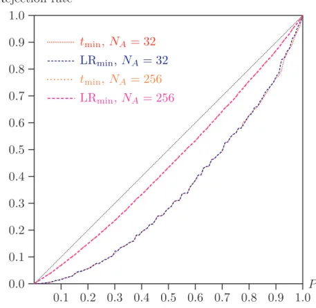
over the full range from 0 to 1. See Davidson and MacKinnon (1998) for a discussion
of P value plots, in which is plotted the CDF of the P value for the test.
0.1 0.2 0.3 0.4 0.5 0.6 0.7 0.8 0.9 1.0 0.0 0.1 0.2 0.3 0.4 0.5 0.6 0.7 0.8 0.9 1.0 ... ... ... ... ... ... ... ... ... ... ... ... ... ... ... ... ... ... ... ... ... ... ... ... ... .... ... tmin, NA = 32 ... ... ... ... ... ... ... ... ... ... ... ... ... ... ... ... ... ... ... ... ... ... ... ... ... ... ... ... ... ... ... ... ... ... .... ... LR min, NA= 32 ... ... ... ... ... ... ... ... ... ... ... ... ... ... ... ... ... .... ... tmin, NA = 256 ... ... ... ... ... ... ... ... ... ... ... ... ... ... ... ... ... ... ... ... ... ... ... ... ... ... .... ...LRmin, NA= 256 ... ... ... ... ... ... ... ... ... ... ... ... ... ... ... ... ... ... ... ... ... ... ... ... ... ... ... ... ... ... ... ... ... ... ... ... ... ... ... P Rejection rate
Two sample sizes are shown: NA = 32 and NA = 256. In the latter case, it is hard
to see any difference between the plots for the two statistics, and even for the much smaller sample size, the differences are plainly very minor indeed.
In the experimental setup that gave rise to Figure 1, it was possible to cover the full range of the statistics, since, even when there was nondominance in the sample, we could evaluate the statistics as usual, obtaining negative values. This was for illustrative purposes only. In practice, one would stop as soon as nondominance is observed in the sample, thereby failing to reject the null hypothesis.
It is clear from bothTable 1andFigure 1that the asymptotic tests have a tendency to
underreject, a tendency which disappears only slowly as the sample sizes grow larger.
This is hardly surprising. If the point of contact of the two distributions is at z = z0,
then the distribution of t(z0) and LR1/2(z0) is approximately standard normal. But
minimising with respect to z always yields a statistic that is no greater than one
evaluated at z0. Thus the rejection probability can be expected to be smaller, as we
observe.
We now consider bootstrap tests based on the minimised statistics. In bootstrapping, it is essential that the bootstrap samples are generated by a bootstrap data-generating process (DGP) that satisfies the null hypothesis, since we wish to use the bootstrap in order to obtain an estimate of the distribution of the statistic being bootstrapped under the null hypothesis. Here, our rather artificial null is the frontier of nondominance, on
which the statistics we are using are asymptotically pivotal, by Theorem 3.
Since the results we have obtained so far show that the two statistics are very similar even in very small samples, we may well be led to favour the minimum t statistic on the basis of its relative simplicity. But the procedure by which the empirical likelihood ratio statistic is computed also provides a very straightforward way to set up a suitable bootstrap DGP. Once the minimising z is found, the probabilities (14) are evaluated
at that z, and these, associated with the realised sample values, the yA
t and the yBs ,
provide distributions from which bootstrap samples can be drawn.
The bootstrap DGP therefore uses discrete populations, with atoms at the observed values in the two samples. In this, it is like the bootstrap DGP of a typical resampling
bootstrap. But, as in Brown and Newey (2002), the probabilities of resampling any
particular observation are not equal, but are adjusted, by maximisation of the ELF, so as to satisfy the null hypothesis under test. In our experiments, we used bootstrap DGPs determined in this way using the probabilities (14), and generated bootstrap samples from them. Each of these is automatically discretised in the tails, since the “populations” from which they are drawn have atoms in the tails. For each bootstrap sample, then, we compute the minimum statistics just as with the original data. Boot-strap P values are then computed as the proportion of the bootBoot-strap statistics that are greater than the statistic from the original data.
Table 2 NA α = 0.01 α = 0.05 α = 0.10 32 0.001 0.018 0.051 64 0.003 0.033 0.082 128 0.006 0.049 0.104 256 0.013 0.053 0.106 512 0.010 0.049 0.102 1024 0.010 0.051 0.100
Rejection probabilities, bootstrap tests, base case, α = nominal level
are given only for the empirical likelihood statistic, since the t statistic gave results that were indistinguishable.
It is not necessary, and it would have taken a good deal of computing time, to give results for sample sizes greater than those shown, since the rejection probabilities are
not significantly different from nominal already for NA = 128.
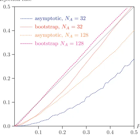
In Figure 2, P value plots are given for NA = 32 and 128, for the asymptotic and
bootstrap tests based on the empirical likelihood statistic. This time, we show results only for P values less than 0.5.
In the bootstrap context, if there is nondominance in the original samples, no boot-strapping is done, and a P value of 1 is assigned. If there is dominance in the original samples, an event which under the null has a probability that tends to one half as the sample sizes tend to infinity, then bootstrapping is undertaken; each time the boot-strap generates a pair of samples without dominance, since the bootboot-strap test statistic would be negative, and so not greater than the positive statistic from the original sam-ples, this bootstrap replication does not contribute to the P value. Thus a bootstrap DGP that generates many samples without dominance leads to small P values and frequent rejection of the null of nondominance.
From thefigure, we see that, like the asymptotic tests, the bootstrap test suffers from
a tendency to underreject in small samples. However, this tendency disappears much more quickly than with the asymptotic tests. Once sample sizes are around 100, the bootstrap seems to provide very reliable inference. This is presumably related to the fact that the bootstrap distribution, unlike the asymptotic distribution, is that of the minimum statistic, rather than of the statistic evaluated at the point of contact of the two distributions.
We now look at the effects of altering the amount of discretisation in the tails of the
distributions. In Figure 3 are shown P value plots for the base case with NA = 128,
for different amounts of agglomeration. Results for the asymptotic test are in the left panel; for the bootstrap test in the right panel. It can be seen that, for the asymptotic
test, the rejection rate diminishes steadily with z− over the range [0.01, 0.10], where
0.1 0.2 0.3 0.4 0.5 0.0 0.1 0.2 0.3 0.4 0.5 ... ... ... ... ... ... ... ... ... ... ... ... ... ... ... ... ... ... ... ... ... asymptotic, N A = 32 ... ... ... ... ... ... ... ... ... ... ... ... ... ... ... ... ... ... ... ... ... ... ... .. ... bootstrap, NA= 32 ... ... ... ... ... ... ... ... ... ... ... ... ... ... ... asymptotic, NA = 128 ... ... ... ... ... ... ... ... ... ... ... ... ... ... ... ... ... ... ... ... ... ... ... ... ... ... .... ...bootstrap NA= 128 ... ... ... ... ... ... ... ... ... ... ... ... ... ... ... ... ... ... ... ... ... ... ... ... ... ... ... ... ... ... ... ... ... ... ... ... ... ... ... P Rejection rate
Figure 2: P value plots for asymptotic and bootstrap tests
0.1 0.2 0.3 0.4 0.5 0.0 0.1 0.2 0.3 0.4 0.5 ... ... ... ... ... ... ... ... ... ... ... ... ... ... ... ... ... ... ... ... ...z− = 0.10 ... ... ... ... ... ... ... ... ... ... ... ... ... ... ...z− = 0.08 ... ... ... ... ... ... ... ... ... ... z− = 0.05 ... ... ... ... ... ... ... ... ... ... ... ...z− = 0.03 ... ... ... ... ... ... ... .. ...z− = 0.01 ... ... ... ... ... ... ... ... ... ... ... ... ... ... ... ... ... ... ... ... ... ... ... ... ... ... Asymptotic 0.1 0.2 0.3 0.4 0.5 0.0 0.1 0.2 0.3 0.4 0.5 ... ... ... ... ... ... ... ... ... ... ... ... ... ... ... ... ... ... ... ...z− = 0.10 ... ... ... ... ... ... ... ... ... ... ... ... ... ... ...z− = 0.08 ... ... ... ... ... ... ... ... ... ... z− = 0.05 ... ... ... ... ... ... ... ... ... ... ... ...z− = 0.03 ... ... ... ... ... ... ... ... ...z− = 0.01 ... ... ... ... ... ... ... ... ... ... ... ... ... ... ... ... ... ... ... ... ... ... ... ... ... ... Bootstrap
Figure 3: Varying amounts of discretisation; base case, NA = 128
entirely as expected, in accord with the discussion in Section 4. For values of z− in
0.1 0.2 0.3 0.4 0.5 0.0 0.1 0.2 0.3 0.4 0.5 ... ... ... ... ... ... ... ... ...asymptotic ... ... ... ... ... ... ...bootstrap ... ... ... ... ... ... ... ... ... ... ... ... ... ... ... ... ... ... ... ... ... ... ... 0.1 0.2 0.3 0.4 0.5 0.0 0.1 0.2 0.3 0.4 0.5 ... ... .... ... asymptotic ... ... ... ... ...bootstrap ... ... ... ... ... ... ... ... ... ... ... ... ... ... ... ... ... ... ... ... ... ... ... ... ... ...
Figure 4: Alternative configurations, NA = 64, z− = 0.1
The base case we have considered so far is one in which B dominates A substantially except at one point in the middle of the distribution. We now consider two other configurations, the first in which the two distributions still touch in the middle, but the dominance by B is less elsewhere. The cumulative probabilities at the upper limits of the eight segments in this case are 0.1, 0.2, 0.3, 0.5, 0.6, 0.7, 0.8, and 1.0. The second configuration has the two distributions touching twice, for values of z equal to 0.25 and 0.75. The cumulative probabilities are 0.10, 0.25, 0.35, 0.45, 0.55, 0.75, 0.85, and
1.00. Results are shown in Figure 4, with z− set to 0.1, and N
A = 64 and NB = 43.
The tests are based on the minimum t statistic. As usual, the empirical likelihood statistic gives essentially indistinguishable results.
For both configurations, all the tests are conservative, with rejection probabilities well below nominal in reasonably small samples. In the second configuration, in which the distributions touch twice, the tests are more conservative than in the first configuration. In both cases, it can be seen that the bootstrap test is a good deal less conservative than the asymptotic one. However, in all cases, the P value plots flatten out for larger values of P , because the P value is bounded above by 1 minus the proportion of bootstrap samples in which there is nondominance. In these two configurations, the probability of dominance in the original data, which is the asymptote to which the P value plots tend, is substantially less than a half.
Another configuration that we looked at needs no graphical presentation. If both populations correspond to the uniform distribution on [0, 1], rejection of the null of nondominance simply did not occur in any of our replications. Of course, when the distributions coincide over their whole range, we are far removed from the frontier of the null hypothesis, and so we expect to have conservative tests.
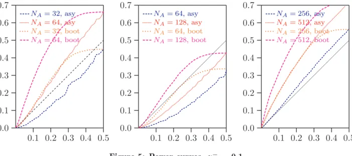
We now turn our attention to considerations of power. Again, we study two con-figurations in which population B dominates A. In the first, we modify our base
configuration slightly, using as cumulative probabilities at the upper limits of the seg-ments the values 0.03, 0.13, 0.20, 0.40, 0.47, 0.57, 0,70, and 1.00. There is therefore clear dominance in the middle of the distribution. The second configuration uses cu-mulative probabilities of 0.1, 0.2, 0.3, 0.4, 0.5, 0.6, 0.7, and 1.0. This distribution is uniform until the last segment, which has a much greater probability mass than the others.
In Figure 5, various results are given, with those for the first configuration in the left-hand panel and for the second in the two right-hand panels. Both asymptotic and
bootstrap tests based on the minimum t statistic are considered, and z− is set to 0.1.
There is nothing at all surprising in the left-hand panel. We saw in Figure 2 that,
with the base configuration, the asymptotic test underrejects severely for NA = 32
and NB = 19. Here, the rejection rate is still less than the nominal level for those
sample sizes. With the base configuration, the bootstrap test also underrejects, but less severely, and here it achieves a rejection rate modestly greater than the significance
level. For NA = 64 and NB = 43, the increased power brought by larger samples is
manifest. The asymptotic test gives rejection rates modestly greater than the level, but the bootstrap test does much better, with a rejection rate of slightly more than 14% at a 5% level, and nearly 28% at a 10% level.
0.1 0.2 0.3 0.4 0.5 0.0 0.1 0.2 0.3 0.4 0.5 0.6 0.7 ... ... ... ... ... ... ... ... ... ... ... ... ... ... ...NA= 32, asy ... ... ... ... ... ... ... ... ... ... ... ... ... ... ... .. ...NA= 64, asy ... ... ... ... ... ... ... ....NA= 32, boot ... ... ... ... ... ... ... ... ... ... ... ... ... ... ... ...NA= 64, boot ... ... ... ... ... ... ... ... ... ... ... ... ... ... ... ... .. 0.1 0.2 0.3 0.4 0.5 0.0 0.1 0.2 0.3 0.4 0.5 0.6 0.7 ... ... ... ... ... ... ... ... ... ... ... ...NA= 64, asy ... ... ... ... ... ... ... ... ... .. ...NA= 128, asy ... ... ... ... ... ... ....NA= 64, boot ... ... ... ... ... ... ... ... ... ... ...NA= 128, boot ... ... ... ... ... ... ... ... ... ... ... ... ... ... ... ... ... .. 0.1 0.2 0.3 0.4 0.5 0.0 0.1 0.2 0.3 0.4 0.5 0.6 0.7 ... ... ... ... ... ... ... ... ... ... ... ... ... ... ... ... ... ... ...NA= 256, asy ... ... ... ... ... ... ... ... ... ... ... ... ... ... ... ... ... ...NA= 512, asy ... ... ... ... ... ... ... ... ....NA= 256, boot ... ... ... ... ... ... ... ... ... ... ... ... ... ... ... ... ...NA= 512, boot ... ... ... ... ... ... ... ... ... ... ... ... ... ... ... ... ... ..
Figure 5: Power curves, z− = 0.1
In the second configuration, power is uniformly much less. If we were to change things so that the null of nondominance was satisfied, say by increasing the cumulative
probability in population B for z around 0.25, then the results shown in Figure 4
indicate that the tests would be distinctly conservative. Here we see the expected counterpart when only a modest degree of dominance is introduced, namely low power.
Even for NA = 128, the rejection rate of the asymptotic test is always smaller than the
rapidly in larger samples, although rejection rates comparable to those obtained with
the first configuration with NA = 64 are attained only for NA somewhere between 256
and 512.
The possible configurations of the two populations are very diverse indeed, and so the results presented here are merely indicative. However, a pattern that emerges consistently is that bootstrap tests outperform their asymptotic counterparts in terms of both size and power. They are less subject to the severe underrejection displayed by asymptotic tests even when the configuration is on the frontier of the null hypothesis, and they provide substantially better power to reject the null when it is significantly false.
Conventional practice often discretises data, transforming them so that the distribu-tions have atoms at the points of a grid. Essentially, the resulting data are sampled from discrete distributions. A few simulations were run for such data. The results were not markedly different from those obtained for continuous data, discretised only in the tails. The tendency of the asymptotic tests to underreject is slightly less marked, because the discretisation means that the minimising z is equal to the true (discrete)
z0 with high probability. However, the lumpiness observed when the two sample sizes
have a large greatest common divisor is very evident indeed, and prevents simulation results from being as informative as those obtained from continuous distributions.
9. Illustration using LIS data
We now illustrate briefly the application of the above methodology to real data using
the Luxembourg Income Study (LIS) data sets5 of the USA (2000), the Netherlands
(1999), the UK (1999), Germany (2000) and Ireland (2000). The raw data are treated
in the same manner as in Gottschalk and Smeeding (1997), taking household income
to be income after taxes and transfers and using purchasing power parities and price
indices drawn from the Penn World Tables6 to convert national currencies into 2000
US dollars. As in Gottschalk and Smeeding (1997), we divide household income by
an adult-equivalence scale defined as h0.5, where h is household size. All incomes are
therefore transformed into year-2000 adult-equivalent US dollars. All household obser-vations are also weighted by the product of household sample weights and household size. Sample sizes are 49,600 for the US, 5,000 for the Netherlands (NL), 25,000 for the UK, 10,900 for Germany (GE) and 2,500 for Ireland (IE).
This illustration abstracts from important statistical issues, such as the fact that the LIS data, like most survey data, are actually drawn from a complex sampling structure with stratification and clustering. Note also that negative incomes are set to 0 (this
5 See http://lissy.ceps.lu for detailed information on the structure of these data. 6 See Summers and Heston (1991) for the methodology underlying the computation of
affects no more than 0.5% of the observations), and that we ignore the possible presence of measurement errors in the data.
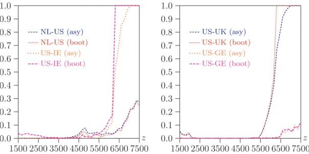
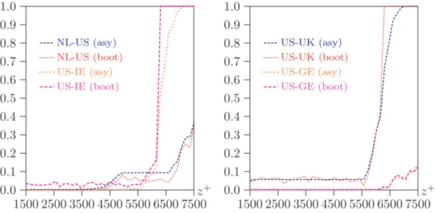
Figure 6graphs the P values of tests of the null hypothesis that FA(z) ≤ FB(z) against
the alternative that FA(z) > FB(z) at various values of z over a range of $1500 to
$7500, for various pairs of countries, and for both asymptotic and bootstrap tests. (Distribution A is the first country that appears in the legends in the Figure.) In all
cases, bootstrap tests were based on 499 bootstrap samples. We set z− to $1500 and
z+ to $7500 since these two bounds seem to be reasonable enough to encompass most
of the plausible poverty lines for an adult equivalent ($1500 is also where we are able to start ranking the UK and the US). The asymptotic and bootstrap P values are very close for the comparisons of the US with either Germany or the UK. The bootstrap P values are slightly lower than the asymptotic ones for the NL-US comparison and somewhat larger for the US-IE one. These slight differences may be due to the smaller NL and IE samples. Although the differences are not enormous, they are significant enough to make bootstrapping worthwhile even if one is interested only in point-wise tests of differences in dominance curves.
1500 2500 3500 4500 5500 6500 7500 0.0 0.1 0.2 0.3 0.4 0.5 0.6 0.7 0.8 0.9 1.0 ... ... ... ... ... ... ... ...NL-US (asy) ... ... ... ... ... ...NL-US (boot) ... .. .... .... .. ... .... ... ... ... ... ... ...US-IE (asy) ... ... ... ... ... ... ... ... ... ... ... ... ... ... ... ... ... ... ... ... ... ... ... ... ...US-IE (boot) z 1500 2500 3500 4500 5500 6500 7500 0.0 0.1 0.2 0.3 0.4 0.5 0.6 0.7 0.8 0.9 1.0 ......... ... ... ... ... ... ... ... ... ... ... ... ... ... ... ... ... ... ... ... ... ... ... ... ... ... ...US-UK (asy) ... ... ... ... ... ... ... ... ... ... ... ... ... ... ... ... ... ... ... ...US-UK (boot) ... ...US-GE (asy) ... ... ...US-GE (boot) z Figure 6: P values for dominance at given points
Figure 7 presents the results of similar tests but this time over intervals ranging
from $1500 to z+. The null hypothesis is therefore that F
A(z) ≤ FB(z) for at least
some z in [$1500, z+] against the alternative that F
A(z) > FB(z) over the entire range
[$1500, z+]. For the NL-US comparison, note first that ˆF
US(z) is always lower than
ˆ
FNL(z) but that the difference between the two empirical distribution functions is small
for z between around $4800 to about $10000. Although it is therefore difficult to reject
the null hypothesis of nondominance for much of the range of z+ values, the bootstrap
P values are significantly lower than their asymptotic counterparts, as is to be ex-pected, given the greater power of the bootstrap test procedure seen in the simulation