Rapport de recherche
Does IMF Induce Political Business Cycles?
An Empirical Analysis on
Latin America’s Indebted Countries
Rendu par
Marta Bastoni
Directeur de recherche
Index
Index... ii
Table index ... iii
Abstract ... iv
I. Introduction... 1
II. A review of the literature on Political Business Cycles... 4
Opportunistic models ... 5 Partisan models ... 8 Context-conditional models... 10 The IMF ... 12 Conditionality ... 15 III. Data ... 16
IV. Theoretical Analysis... 21
Testing the presence of Political Business Cycles... 21
The moral hazard problem ... 23
Does election proximity matter in IMF behavior?... 24
V. Empirical analysis ... 25
Test for political Business Cycles... 25
Government Moral Hazard and the endogeneity problem... 30
Are elections influencing the behavior of IMF? ... 34
VI. Conclusions ... 38
Bibliography... 40
Annex ... 43
Table index
Table 1 : Growth monetary base (Original Version) 25
Table 2: Growth monetary base (Revised Version) 27
Table 3 Deficit over GDP 28
Table 4: Government budget deficit :Moral Hazard 32
Abstract
This research (1) investigates the presence of political business cycles in Latin America by looking at two major economic variables (money growth and budget deficits) and (2) studies the influence of the IMF on economic decisions made by political incumbents from 1976 to 1997.
Our research answers three main questions. First, we determine the presence of political business cycle in a dataset of 16 Latin American countries. Second, we ask ourselves whether the presence of IMF credit is increasing the willingness of the politicians to use economic policy instruments to maneuver the economy with the purpose of being reelected, that is, whether there is a Moral hazard issue from the government side. The third point is related to the second one, but it reverts the causality: the attention now is on whether the proximity to the election is affecting the behavior of IMF, namely the decision of granting new credit.
The analysis shows a significant presence of political business cycles on the government budget (but not on money growth) and a quite robust evidence of moral hazard from the government side, to the extent that access to credit seems to exacerbate the willingness of a government to distort the economic cycle for electoral reasons. For what concerns the behavior of the fund on election proximity, although the Fund tries to minimize the default’s risk by cautiously approving less new credit to countries that have already heavily borrowed in the past from the Fund, the credit authorized to right-wing parties results to be consistently higher.
I. Introduction
Political business cycles (PBC) have been largely studied since the 70’s and the literature on this subject has grown enormously since then, adding several extensions and inducing a large critical debate between economists about the causes and the solutions as well. The question is interesting because the standard theory on the business cycle, which abstracts from political considerations, is often incapable of explaining the cyclical behavior of most economic variables. For example, Ellery, Gomes, and Sachsida (2002) assert that the economic cycle in Brazil is not explicable by the theory of real business cycle.
So far the political business cycle literature has mostly focused on OECD countries. Moreover, the existing literature has never taken in consideration the role of an international lender like the IMF and the influence that an international organization could exert on the political business cycle of an indebted country.
Compared to the current literature, the dataset that we consider includes Latin American countries. These countries are from severely to moderately indebted with international institutions. Credit availability is therefore a crucial issue for those countries and puts the IMF in a strong position for negotiations.
First, we determine the presence of pre-electoral business cycles by looking at two economic variables: the government budget over GDP ratio and the money growth. This objective is pursued following the empirical strategy in Alesina, Roubini and Cohen (1997), who suggest two different regressions, one for each economic policy instruments, in order to investigate the relation between each variable and the pre-electoral dummy variable. As suggested by Alesina Roubini and Cohen (1997), the regression is done on a cross-country panel dataset, where (1) the dependent variable, the monetary growth is regressed on its lags and electoral dummy, and (2) the variation in government budget is regressed on the change in unemployment rate, on GDP growth, on the variation in the ratio of debt service over GDP and on the pre-electoral dummy variable
The second part of our analysis is whether the IMF aggravates the Moral Hazard problem in the recipient country before an election. The policymakers in the recipient country are obviously interested in having a good economic performance before the elections in order to be reelected. What is to determine is if the presence of IMF credit is helping politicians seeking power or not. The empirical analysis on this topic is related to the empirical paper proposed by Dreher and Vaubel (2004). The fiscal policy instrument is regressed on its lag, on the IMF exhaustion quota during the previous period, on the new net credit accorded by the Fund during the previous period, on the pre-electoral dummy variable, and on two economic indicators, namely inflation and GDP growth for the previous period.
The third part of our work is related to the previous, but reverses the causality: the attention now is on whether the proximity to the election is affecting the behavior of IMF. In order to answer to this question, following Dreher and Vaubel (2004) we regress the new net credit accorded by IMF on two economic policy instruments, on the electoral dummies, on a series of internal economic indicators, such as namely inflation, the country’s net account balance, the GDP growth and the government consumption. Moreover, the regression takes in consideration another sets of variable as regressors, namely variables that show the composition of debt and the quality of the resources of the country. Those variables are the ratio short-term foreign debt over long-term foreign debt, international reserves over money supply, and the debt service.
The work is organized as follows: In Section II, there will be a review of the literature on the subject, both on a theoretical level and on an empirical one. Section III will be devoted to a short description of the dataset used in the empirical analysis. In Section IV there will be a description of the analysis to perform, which results are going to be in Section V. In Section VI, conclusions will be drawn.
II. A review of the literature on Political Business Cycles
Political Economy investigates the relations between the institutional structure of a given country (such as, the form of government and the degree of democracy and transparency) and economic outcomes. A particular field of interest in the political economy literature studies the Political Business Cycles (PBC). The literature studies the behavior of policymakers who may have an incentive to artificially inflate growth before election, as well as the behavior of electors.
Shi and Svensson (2003) give a definition of political budget cycles, as being “a fluctuation” in the budget aggregate that is caused by election proximity. By extension, the PBC literature studies the economic cycles (that is, fluctuation in real economy variables, inflation or monetary variables) induced by the political cycles
The first model on political cycles by Nordhaus and Hibbs (1975) is based on the strong hypothesis of adaptive expectations and retrospective voting. Rational expectation models were introduced around ten years later by different authors. This new literature on PBC can be divided in electoral cycle models (also called opportunistic models) and partisan cycles models. The difference between these two strands of literature is given by the motivations of politicians: in opportunistic models, politicians are office-seeking and their only objective is to maximize the probability of winning; in partisan models, policy-makers care about the policies that will be implemented after the election. Inside those two categories that will be shortly illustrated, research comes to some common agreement on the direction to pursue, but not always on the ways to get there. After describing these two types of approach, I will review context-conditional models.
Opportunistic models
Models in which policy makers are seeking re-election for themselves, no matter what it takes in term of policy, are called electoral or opportunistic.
The most relevant ones are the models of Rogoff (1990), Rogoff, Sibert (1989) and Persson, Tabellini (1990), all of them having different approaches. All those models are hypothesizing rational expectations. In Persson Tabellini (1990), the information about the politicians’ competence is imperfect and electors are rational. Electors appreciate price stability and output growth and vote for the most competent candidate.
The policymaker has an interest in obtaining a good economic performance to signal her competence as policymaker. The measure of competence is persistent, which means that policymakers have an incentive to manipulate the economy before elections to signal their competence after the election (in fact only competence after the election matters if voting is prospective). The incumbents therefore take advantage of a short-term Phillips curve to attain a better economic performance. In every period electors know the measure of competence of the past period, but they cannot infer the one of the current year, since inflation is known only with one period of delay.
This model gives rise to both pooling equilibria (in which it is not possible for electors to discriminate between level of competence) and separating equilibria, in which policymakers with different competence choose different strategies. The way to signal high level of competence is to achieve a level of economic growth that could not be attained by an incompetent policy-maker. This implies choosing a higher than optimal level of inflation. The result is that if the incumbent is a competent policymaker, there will be a political business cycle, but not otherwise.
The model of Rogoff and Sibert (1989) and Rogoff (1990) the competence is captured by a persistent measure of efficiency in the production of public goods. Policymakers have therefore an incentive of signaling competence in order to be reelected by increasing the provision of public good. The intuition for this result is the following. Only a competent policy-maker is willing to worsen the budget situation with the notion that only someone who is very competent would put himself in that situation. Compared to a competent politician, an incompetent policy-maker who worsens the budget has to rely on distortionary taxation to balance the budget after the election. Assuming that aggregate welfare enters the objective of both types of politicians, an incompetent candidate does not mimic what the competent does.
In Rogoff and Sibert (1989), government spending is financed by seignorage, which is distortionary, or by less-visible debt. Every policymaker with the exception of the most incompetent chooses to boost pre-electoral budget spending using seignorage. The good pre-electoral economic performance is a signal of competence that cannot be evaluated directly, but only inferred from present economic situation.
In those models it always exists an equilibrium in which we can separate competent and incompetent policymakers (separating equilibrium), even though it is not possible to rule out a pooling equilibrium, that is, an equilibrium where all types act in the same way, with no possibility of discerning competence. It is clear that this model provides indeterminate solutions, if no further assumptions are made.
In a second specification, Rogoff (1990) adds some more refinement to the government budget constrains, discriminating between government spending, more visible to the public, and “government investments”, less visible. Under election, competent policymakers have the incentive or reallocating resources from less visible investment to highly visible spending. The cycle appears only in some monetary and fiscal policies, more than real outcomes.
Drazen (2001) reviews the literature on PBC and argues that the “driving force” of the cycle does not have to be found out in the monetary policy, as in the model by Persson and Tabellini, rather in the fiscal policy. This is why in this research we mostly focus on fiscal variables.
Partisan models
In partisan models, policymakers differ according to their preferences. The model of Alesina (1997) pioneered the rational expectations in a partisan model. The starting assumption is that political parties have economic priorities that are set on an ideological basis. Left parties focus more on growth and unemployment, while partially disregarding effects on inflation. Right parties, on the other side, are more aware of the level of prices than unemployment. Each party fixes a desired level of inflation, πi, with i = L, R.
The asymmetry implied in the model is summarized by the condition πL≥ πR ≥0, that is,
the objective level of inflation of the right party is lower that the left one. Consequently, the expected inflation before election will be a weighted average of πL and πR, with the
respective probability of victory at election as weights.
Voters therefore will proceed to wage setting with an expected inflation that is systematically too high or too low compared with the ex-post actual level.
This discrepancy results in an “artificial” cycle: in the case of a left party elected, actual inflation will be higher than expected. The positive unexpected shock of inflation will increase the demand for labor and decrease unemployment. The following period, however, expectations will adjust and rate of growth of production will remain constant. In case of a right party elected, on the other hand, there will be a level of inflation lower than expectations. This will induce a one-period reduction in the demand for labor (more expensive) and therefore an increase in the unemployment rate.
The theory of partisan cycle will therefore predict an economic expansion (accompanied by higher than expected inflation), during the year following the election of a left party and an economy growing less than its natural rate (accompanied by inflation lower than expectations) the year after the elections of a right party.
After checking for the presence of political budget cycles, next step is to test whether the IMF is having an interest in lending more money to countries that are already indebted with international lenders, and more specifically, whether this interest actually pairs with an increase in the quantity of money lent in proximity of electionary periods.
Bearing this in mind the partisan-cycles relevant variables will be an insightful addition to control. However, as Kraemer (1997) noted in his paper “Electoral budget cycles in Latin America and the Caribbean: incidence, causes and political futility”, Latin American governments are in practice less ideologically defined, compared with OECD countries, and that it is realistic to expect more volatility in the partisan structure.
Moreover, Shi and Svensson (2003) remark that up to now, no paper that seeks for evidence of PBC in developing countries uses partisan cycles. In fact, even if those kind of model result to be successful in OECD countries, “the [partisan] distinction frequently does not exhibit the typical Western left-right pattern”. For this reason partisan
considerations will be dealt more as a factor to control for, rather than a pattern for PBC. In the next subsection I will introduce another set of models on political budget cycles, the context conditional models.
Context-conditional models
The first electoral models do not pay enough attention to the context. As a result, recent literature on PBC has introduced new dimensions of analysis, such as:
- Degree of openness of the economy to an international contest - Economic policy conjuncture and restrains (fixed exchange rate…) - Form of government and structure of power organization
- Repeated game strategy problems (election will be held again..)
The above features have been singularly taken in account by countless articles. The context-conditional literature is a heterogeneous collection of models that explores election influence in a more complex way.
The environment conditions become relevant part of the interaction between the players in the model. Incumbents’ autonomy of decision on matter of political economy might be constrained by the context in which the economy is operating.
The review on this literature will focus on papers that somehow will give some insight on the question posed, both for what concerns the methodology and the choice of variables. Bernard and Leblang (1999) argue that the constraint of fixed exchange rate would make incumbent lose their ability of controlling monetary policy and, consequently, signaling their competence by engineering political budget cycles They argue also that a policymaker will voluntarily commit to a fixed exchange rate regime only under particular conditions in the domestic electoral and legislative institutions. Furthermore, they state that policymaker could make the currency float before the election, fixing it after the election. Their results show that the electoral cycle variable is not significant in the determination of deciding whether accept fixed exchange rate or not.
Only if the cost of an eventual electoral defeat is not too high and the election timing can be “adjusted” endogenously, policymakers will agree to lose the possibility of manipulating monetary policy and accept fixed exchange rate.
Clark and Hallemberg (2000) seek to identify “how the interaction of the international environment with the domestic political institutions constrains a government’s ability to engineer pre-electoral macroeconomic expansion”. They apply the logic of the Mundell-Fleming model by hypothesizing that under fixed exchange rate the governments still have the possibility of signaling competence before elections by using the fiscal policy channel. Pre-electoral budget expansion is the theoretical result, when exchanged rate are fixed.
The study of Brender and Drazen (2004) aims at verifying if there is any connection between the youth of a democracy and political budget cycles. The empirical evidence that they collect suggests that newer democracies suffer of political budget cycles more than older ones.
I will introduce a brief ensemble of facts on the International Monetary fund that are necessary to fully understand the analysis.
The IMF
1Traditionally, the IMF has been seen as the “lender of last resort”, for countries with strong macroeconomic imbalances (high inflation, instable exchange rate, recession, high debt, or all of them together ).
The Articles of Agreement set the legal foundation for the action, as well as the mission of the Fund, that is to promote stability of the exchange rate system, of the balance of payments, to assist countries in the implementation of new systems of payments, to promote growth in international trade.
The IMF is lending money to member countries under several programs, specifically designed for the particular circumstances faced by the member countries, for instance, the poverty reduction facility or the many geography-related ones. The primary lending program for IMF is the Stand-By Facility, a short-term non-concessional loan designed to solve liquidity problems. Other non-concessional loans are the Extended Fund Facilities, which are usually covering a three years period and are designed to implement structural programs of reform.
The process starts when the government of the country that wants to enter in an IMF program signs a “letter of intent” addressed to the IMF Executive Board. This is a document where there are stated the guidelines on the economic policy that the policymakers are willing to undergo.
This letter in itself is not legally binding for the requesting country, nevertheless policymakers have a strong incentive not to loose their credibility in committing themselves to unrealistic constraints. The letter can be as well the result of preliminary informal discussion with the IMF staff.
1 This paragraph relies on the information available on the IMF website www.imf.org , unless otherwise
The sense of this document is basically to agree on the economic path to follow in order to pursue an economic balance. The letter of intent has to be evaluated and approved by the Executive board. The disbursement of money doesn’t necessarily take place in only one stand, but it can be granted in several parts, especially the Extended Fund Facilities, due to the length of the program. The disbursement of the loan has to be accompanied by a control system, to prevent diversion of the resources allocated to specific projects. In order to prevent misuse of the loans, a process of periodical evaluation of the Country’s behavior is put in place. Here, the IMF estimates the capacity of the country to fulfill its commitments and monitors the progresses accomplished by the government. On this matter, the fourth Article of Agreement of the International Monetary Fund gives the legal and operational framework for the activity of surveillance. Each member country has to periodically provide to the Fund the necessary information to allow the accurate examination of the economic and structural situation of the country.
According to Article IV consultations usually take place once a year, no matter if the member country is having a pending situation with the fund or not.
On the base of the Consultations, the Executive Board decides on the concession of the following part of the loan.
Unfortunately the work of the Fund is highly sophisticated and delicate for the very nature of the actors involved and the interests they are bearing. The order of problems encountered in the process is quite vast and articulated:
• Non-compliance • Bias in accession
The periodic evaluation performed by IMF on recipient countries in order to assess the fulfillment of the requirement demanded by the international community (compliance) reserves often sour surprises: the number of countries that do not comply is high and the percentage of success of Fund’s program is quite low. Joyce (2003) reviews several authors that approached the subject.
For what concern accession, the process of money-lending is not all the time as transparent, nor as successful as we wish to think and there is a relevant part of the decision on whether giving credit or not to a country that is highly discretionary.
On this matter, Joyce cites Thacker (1999) and Barro and Lee (2003) that found evidence that access to IMF program is biased towards countries whose vote is aligned with the one of United States, in United Nations voting procedures.
The study of Dreher and Vaubel (2004) arrives as well to quite important conclusions: they perform a ‘cross-country’ analysis on the effects of FMI and World Bank on political budget cycles. The empirical analysis suggests that there is a greater quantity of loans disbursed before elections.
Searching for the influence of IMF on the political business cycles, it is crucial to find a rational motivation for the Monetary Fund to affect somehow a country’s electoral equilibrium.
Vaubel (1986) introduces an interesting explanation, based on public choice theory. He suggests that IMF bureaucrats, like politicians, are interested in pursuing personal objectives, which are not necessarily shared by the establishment or by the voters. Moreover, Dreher (1993) cites Vaubel (1991), reaching the conclusion that there is an interest of IMF bureaucrats to increase the amount of money borrowed to a recipient country, because their position of prestige inside the structure “rises with the amount of money lent and the stringency of the conditionality”. A motivation of this kind would explain an eventual increase of money lent in election period: Personal objectives would enter in the process of decision of lending money to member countries, affecting the process. The IMF would therefore have the chance to expand its basin of credit over the physiological necessities of the country.
Conditionality
A relevant characteristic of an international institution’s loan is the presence of conditionality. As stated in the IMF paper “Conditionality in Fund-Supported Programs. Policy Issues” (2001), conditionality is “the linkage of financing to the implementation of economic policies”, that is the introduction of economic policy terms for the recipient countries. The country can access to the full amount of loan granted, provided that some conditions on economic policies previously agreed are implemented. The conditions touch usually macroeconomic performance indicators, however they can as well imply more structural reforms, as for example reforms in the banking system or the adoption of a currency board.
The main purpose for conditionality is to ensure that the resources are actually used for the reason why they have been requested and not directed elsewhere.
The same system of conditionality is put under accusation: The need of redesigning the extent and the finality, especially for structural clauses, is felt from the inside of the Fund as well as the outside: A paper prepared by the Fund in 2001 expresses the perplexities on the effectiveness and the necessity of conditionality. Moreover Drazen (2002) arrives to the conclusion that conditionality plays a role only in the absence of political agreements over objectives in the recipient country.
Finally, it is interesting to note that the number of conditionality clauses has been increasing over time, especially after the 1997 Asian Crisis. On the subject, the International Financial Institution Advisory Commission, chaired by Meltzer submitted in 1999 to the US cabinet a report to highlight present problems and suggest future guidelines to the redefinition of international monetary institutions.
III. Data
2The countries that were taken in consideration are 16, all from the Latin America area. The World Bank defines ten of them as “severely indebted countries”.
Those are: Argentina, Bolivia, Brazil, Ecuador, Guyana, Haiti, Honduras, Jamaica, Nicaragua, Peru. Cuba was taken out of the sample, because no data were available to the public from the World Bank source.
The World Bank defines six more countries of the dataset as “moderately indebted”. Those are: Belize, Chile, Colombia, Panama, Uruguay and Venezuela.
St.Vincent et Grenadine and Dominica were taken out of the sample because there was no information available on their electoral history. Being the electoral variable a critic concept of the study, the inclusion of it could corrupt the outcome of the empirical work. The period that was taken in consideration goes from the 1975 to 1997. All the data are annual, and they are not deseasonalized. Here is a description of the series used:
The study is highly based on the use of electoral and partisan dummy variables.
The countries included in the dataset, however, have not always experienced democracy in the period of reference, therefore election, post-election and partisan dummy variables record a “not available” value during period of dictatorship. Moreover, in the panel regression, not available value will not enter in the regression and will not be taken in account. Panel dataset will be therefore unbalanced.
2 In this section I refer several times to one of my most important data source: International Bank for Reconstruction and Development (2000) “World Development Indicators,CD-ROM.” Washington, DC. For simplicity I will refer to the source as “World Bank”.
Overall budget deficit, including grants (% of GDP) -BD
Total expenditure and lending (minus repayments), less current and capital revenue and official grants received. Data are shown for central government only. World Bank definition.
I changed the sign of the series, in order to have some coherence in the terminology. A budget deficit is going therefore to have a positive sign, and a surplus a negative one Utilization of IMF quota. -UQ
The exhaustion of the IMF quota is seen as the total liabilities of the countries, as a percentage of the IMF quota. IMF Definitions. The variable capture the dimension of the total debt of a country toward the IMF. Recall that every country has to deposit a certain amount of money in the Fund. This amount is predetermined and is called quota. Every country has the right under normal agreement to a credit line up to 200% of the quota. However this limit does not include special project financed by the Fund, which are associated with development finalities.
Net change in IMF credit -NNC
“The IMF credit denotes repurchase obligations to the IMF for all uses of IMF resources (excluding those resulting from drawings on the reserve tranche). These obligations, shown for the end of the year specified, comprise purchases outstanding under the credit tranches, including enlarged access resources, and all special facilities (the buffer stock, compensatory financing, extended fund, and oil facilities), trust fund loans, and operations under the structural adjustment and enhanced structural adjustment facilities. Data are in current U.S. dollars” The variable is constructed as the first difference of the IMF credit series. World Bank definition
“GDP measures the total output of goods and services for final use occurring within the domestic territory of a given country, regardless of the allocation to domestic and foreign claims. Gross domestic product at purchaser values (market prices) is the sum of gross value added by all resident and nonresident producers in the economy plus any taxes and minus any subsidies not included in the value of the products. It is calculated without making deductions for depreciation of fabricated assets or for depletion and degradation of natural resources. Data are in constant local currency” Note that this variable is in real terms and the fact that is calculated at “market prices” refers to the fact that the prices used are the prices at which final sales are made on a base year. World Bank definition. Inflation -INF
“Inflation as measured by the consumer price index reflects the annual percentage change in the cost to the average consumer of acquiring a fixed basket of goods and services.” World Bank definition.
Monetary growth -MON
“Average annual growth rate in money and quasi money. Money and quasi money comprise the sum of currency outside banks, demand deposits other than those of the central government, and the time, savings, and foreign currency deposits of resident sectors other than the central government. The change in the money supply is measured as the difference in end-of-year totals relative to the level of M2 in the preceding year.” The variable is capturing the nominal change in the M2 aggregate. World Bank definition. Pre-election Dummy -ELE
A great part of the literature on business cycles relies on the availability of annual data on election. This can create quite an obvious problem of “roughness” and imprecision in the electoral dummy variable created by those data.
In fact, an election held in February will have a different impact on the current period than an election held in November: in this last one, the pre-electionary effect is going to be more powerful.
Thorsten Beck, George Clarke, Alberto Groff, Philip Keefer, and Patrick Walsh (2001) created The Database of political institutions. The month of elections, both executives and legislatives was marked, allowing a more precise specification of the electoral dummy variable: the construction was quite linear: The ratio of the 12 months before the elections that was falling in each period was used, and if a country was having both presidential elections and legislative election an equal weight was given.
The use of 12 months length for the political cycle has been preferred , as suggested by Franzese (2002b), rather than an 18 months length, as used by Dreher and Vaubel (2004) because a longer cycle implicitly calls for a more regular electoral pattern, which is a strong assumption for the dataset used.
Post-election Dummy -POSTELE
Starting from the dummy variable ELE, which capture the fraction of the year falling before the elections, it is possible to construct in the same way another dummy variable that captures the fraction of the solar year that falls after the election event. It is necessary to control for cycles in the fraction of the period that falls after an election.
Partisan Dummy –PARTISAN
The dummy variable PARTISAN is set to be equal to 1 when the party in power is considered to be right-handed, and zero otherwise. It is used to control for partisan differences in the allocation of resources.
Total debt service % GDP -SE
Total debt service is the sum of principal repayments and interest actually paid in foreign currency, goods, or services on long-term debt, interest paid on short-term debt, and repayments (repurchases and charges) to the IMF, as a percentage of GDP. Data are in current U.S. dollars. World Bank Definition.
Share of foreign short-term debt in total foreign debt. -FD
Short-term debt includes all debt having an original maturity of one year or less and interest in arrears on long-term debt. World Bank Definition
Current Account Balance as a percent of GDP -AB
Current account balance is the sum of net exports of goods and services, income, and current transfers. World Bank Definition
IV. Theoretical Analysis
In order to verify the presence of budget political cycles in countries severely to moderately indebted and to test for an eventual effect of the IMF on the political Budget cycle, I will focus on three questions that are highly related to each other:
Testing the presence of Political Business Cycles
The first objective of my analysis will be to test for the presence of PBC in the dataset. In his review of the literature on PBC, Drazen (2000) highlights the academic consensus on the fact that political cycles are to occur in monetary and fiscal policy instruments, rather than in real economic outputs.
In particular, he argues that the “driving force” of PBC should be seen in the fiscal policy. Along the same lines, Shi and Svensson (2003) emphasize that the government’s surplus (or deficit) seems to be more influenced than monetary policy variable by political activities.
In my analysis I test for the presence of Political Business Cycles both in the monetary instrument, namely the money growth, and in the fiscal instrument, namely budget deficit. In order to do this, the literature suggests to run panel regressions of time-series, cross-section data.
The regression on monetary instruments for every single country will then look like this:
0 1 1 2 2 ... 1
it it it n it n n it it
mon =β +βmon − +β mon − + +β mon − +β +ELE + , ε
where ELE is the electoral dummy and mon the monetary growth and its lags. In the empirical part I will add inflation as an ulterior control variable.
The purpose is to test if the coefficient for the election dummy variable is significative and eventually, what is its sign.
For what concerns the test on fiscal policy, I run the following Ordinary Least Squares panel regressions:
0 1 1 2d 3d 4 1d( ) 5 6
it it it it it t it it it
bd =δ δ+ bd − +δ U +δ gr +δ b− r−gr +δ ELE +δ PARTISAN + , v where bd is the annual deficit over GDP, dU is the change in the rate of unemployment, ELE the pre-electoral weighted dummy variable and PARTISAN the dummy variable that signals the government political orientation.
The variable d(rt-grt) is the change in real interest rate minus the output growth rate, then
multiplied by the debt over GDP ratio. This variable is catching the effect of variation of debt servicing cost after acknowledging for the “natural” increase of this variable due to economic growth.
The reason for including such a variable is explained by Alesina Roubini and Cohen (1997): in the 70’s, after the first oil crisis, indebted countries experienced a substantial increase in the amount of interests paid on their debt, dynamic that must be taken in account when analyzing budget deficits. Unfortunately it was not possible for the dataset of interest to construct a coherent variable based on interest rate values. There was in fact no common financial measure between the countries composing the dataset.
This is quite easily understandable: Not all the countries of the dataset had already a complex financial system and there was no standardization of measures. For this reason I decided to use as a measure of the change in debt costs, the difference in the World Bank measure of total debt service as a percentage of GDP.
In this regression, the purpose of the analysis is to test whether the coefficient for the election dummy variable or the partisan dummy variable coefficient are significant, and the sign of the relation.
Note that in this model election dates, unemployment and interest rates are considered as exogenous in this model. The choice of OLS is therefore motivated by its efficiency, since the regression does not give problems of endogeneity.
The moral hazard problem
The second issue to explore is whether or not IMF somewhat aggravates the government moral hazard problem, In other words, we check whether credit availability in the occurrence of economic crises distorts the behavior of policymaker: and their decision to accumulate debt. In fact, IMF liabilities might be perceived as “an insurance against adverse shocks” (Dreher and Vaubel, 2004). This would ultimately lead policymakers to accept higher risks. Even if this is not the object of the present analysis, it highlights the implicit dangers that credit availability may induce. In particular, it suggest that under the election, credit availability may induce by affecting the evaluation of risk from borrowing extra resources.
In order to test whether IMF loans are actually induces moral hazard, I run the following panel regression for the fiscal policy instrument.
0 1 1 2 1 3 4 5 6inf 1 7 1
it it it it it it it it it
bd =β +βbd − +β uq − +β NNC +β ELE +β POSTELE +β − +β gr− +ε ,
where the dependent variable is the budget deficit as a percentage of GDP, UQ is the utilization quota of IMF loans, NNC is the IMF new net non concessional credit , ELE is the pre-electoral dummy variable, INF is the inflation rate and GR is the output growth rate.
The hypothesis to be tested in this case is the significance of the coefficients of the variables UQ and NNC, that is to test whether availability of credit and previous cumulative agreement for credit with IMF do influence government spending.
In this case, a problem of endogeneity arises: the quantity of new net non-conditional debt could in fact depend on the present and past values of budget deficits, as the country’s economic performance is one of the parameters evaluated by the Fund in the concession of loans.The most appropriate estimator to use according to Shi and Svensson (2003) is the Arellano-Bond generalized method of moments methodology, that takes into account the endogeneity problem in a dynamic panel data.
Does election proximity matter in IMF behavior?
After testing for Moral Hazard, the next step is to look at the question on the other side. That is, does the election’s proximity modify the behavior of IMF on lending matters? The question is almost specular to the one posed in the previous section on the moral hazard problem.: On the IMF side, in fact, the proximity to elections in the recipient country could induce the Fund to agree on loan concessions beyond real needs of the recipient country, exploiting the increased demand due to election proximity.
The regression suggested by Dreher and Vaubel (2004) consists in using the new net credit that a country has received from IMF during the year as the dependent variable and regressing it on a set of variables that represent the “instruments” in the hands of policy makers: monetary growth, budget deficit as before and government consumption as a % of GDP. The regression to be tested is the following:
0 1 1 2 3 4
5 1 6 1 7 1 8 1 9 1 10 1
it it it it it
it it it it it it it
NNC NNC ELE POSTELE PARTISAN
UQ inf gr FD AB SE β β β β β β β β β β β ε − − − − − − − = + + + + + + + + + + + +
where the dependent variable is the IMF new net non concessional credit , ELE is the pre-electoral dummy variable, POSTELE is is the post-electoral dummy variable, PARTISAN is the dummy variable that signals the government political orientation, UQ is the utilization quota of IMF loans, inf is the inflation rate, gr is the output growth rate, FD is the foreign short-term debt over total foreign debt, current account balance as a percent of GDP, while SE is the total debt service as a percentage of GDP.
As before, our methodology uses the Arellano Bond estimator, which will be further described in the empirical analysis.
V. Empirical analysis
Test for political Business Cycles
In this section I will run the tests for Political Business Cycles both for the monetary and for the fiscal policy instrument
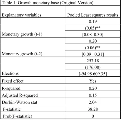
From the initial form of regression suggested by Alesina, Roubini and Cohen (1997), the lags of monetary growth bigger than two were not significant. Furthermore, checking for fixed effects in the sample turned out to have some surprisingly marked differences across countries. In Table 1 I omitted the values of each country’ specific coefficient. The first value is the coefficient, the value in parenthesis is the standard deviation , the values in squared parenthesis are the 95% confidence interval.
Coefficients that are significant at the 10% significant level are marked with a star* next the standard deviation, while coefficients that are significant at the 5% significant level are marked with a double star**.
Table 1: Growth monetary base (Original Version)
Explanatory variables Pooled Least squares results 0.19 (0.05)** Monetary growth (t-1) [0.08 0.30] 0.20 (0.06)** Monetary growth (t-2) [0.09 0.31] 257.18 (176.08) Elections [-94.98 609.35] Fixed effect Yes
R-squared 0.20 Adjusted R-squared 0.15
Durbin-Watson stat 2.04 F-statistic 38.28 Prob(F-statistic) 0
The regression of monetary growth on its lag has a very poor result. The R squared is low, but still acceptable. The coefficients on the two lags of monetary growth are significant and positive. This means that there is some persistency in the series. The coefficient of the election dummy variable ELE is not significant, suggesting that political business cycles do not manifest themselves through money growth.
However, the regression’s R squared is low, which could indicate a problem of misspecification, and more in detail, a problem of omitted variables. It is therefore too early to assess to absence of Political business cycles in the monetary instrument. I will introduce inflation as a control variable for the regression
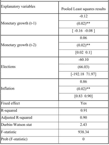
Table 2 shows a second regression, performed starting from the original theoretical formula. Inflation is added to the explanatory variables. This assumption is quite reasonable, since the database is made of highly and moderately indebted countries, and that several between them experienced episodes of high or very high inflation (i.e. Brazil, Argentina, Bolivia).
Table 2: Growth monetary base (Revised Version) Explanatory variables
Pooled Least squares results -0.12 (0.02)** Monetary growth (t-1) [ -0.16 -0.08 ] 0.06 (0.02)** Monetary growth (t-2) [0.02 0.1] -60.10 (66.03) Elections [-192.18 71.97] 0.86 (0.02)** Inflation [0.83 0.90] Fixed effect Yes
R-squared 0.91
Adjusted R-squared 0.90 Durbin-Watson stat 2.43
F-statistic 938.34 Prob (F-statistic) 0
In this regression, the pre-electoral dummy is still not significant, however the regression appears more reasonable for this dataset than the version suggested by Alesina, Roubini, Cohen, at least for what concerns the R squared which has significantly risen
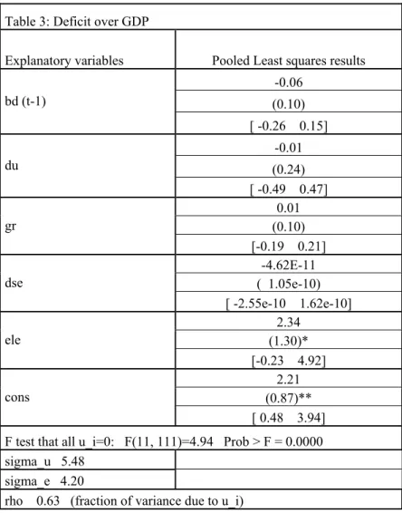
In the test for Political Business Cycles in the fiscal policy, the fixed country effect was not significant; therefore the final model proposed in Table 3 is showing a common intercept.
Table 3: Deficit over GDP
Explanatory variables Pooled Least squares results -0.06 (0.10) bd (t-1) [ -0.26 0.15] -0.01 (0.24) du [ -0.49 0.47] 0.01 (0.10) gr [-0.19 0.21] -4.62E-11 ( 1.05e-10) dse [ -2.55e-10 1.62e-10] 2.34 (1.30)* ele [-0.23 4.92] 2.21 (0.87)** cons [ 0.48 3.94] F test that all u_i=0: F(11, 111)=4.94 Prob > F = 0.0000 sigma_u 5.48 sigma_e 4.20 rho 0.63 (fraction of variance due to u_i)
None of the coefficient is significant: nor the change in the rate of unemployment, nor the coefficient of the output growth, nor the proportion of debt service over GDP.
The pre-electoral dummy is significant at a 10% level of confidence, and positive. This means that an increase of the part of the pre-electoral year in a given period is going to increase the budget deficit of (2.34/12) % for each month, compared to a non-electionary period. This is the confirmation that some sort of political business cycle is showing in the fiscal policy variable. It is important to stress that the coefficient is robust to quite a series of specification.
The F test suggest that in this case a fixed effect estimation is correct.
The autocorrelation matrix does not show any serious pattern of serial correlation of the residuals.
Government Moral Hazard and the endogeneity problem
The tests for the moral hazard are a little more cumbersome in the application.
I will first of all give more information on the variables of interest, and then discuss about the potential implication of variables’ interactions.
The interpretation Dreher and Vaubel (2002) give about the new net non-concessional credit variable insists on the discretion of the quantity of credit received by IMF: once the country quota in the Fund is established (and a maximum amount of credit receivable too) the credit is negotiated for roughly a three to five years frame (see Annex). However, as I already mentioned, the payment of the different parts of the loan is conditional to the accomplishment of some predetermined objectives. It is clear that the quantity of new, net IMF credit toward governments might be affected by values of early deficit, i.e. a non virtuous government budget in period t-1 might have an influence in the credit decisions in t. On the other side, the budget could be swayed most reasonably by the quantity of credit obtained in the previous years by the Fund.
There is a problem of endogeneity that affects the potential results of an OLS analysis: in case of endogeneity, in fact OLS fixed effects methodology produces an estimator that is biased and inconsistent: this problem needs to be taken into account.
The Arellano-Bond GMM estimator uses as the dependent variable the first difference of the variable of interest and uses as instruments for the independent endogenous variables the first difference and the lagged levels of the variable.
The gain from using the Arellano-Bond GMM estimator rather than an instrumental variable one is the better exploitation of the information, which leads to a greater efficiency.
The Arellano- Bond estimator can be performed in one or two steps; the difference is that the two steps procedure optimizes the covariance matrix estimated in the first step and improves the efficiency of the estimator. However, Arellano and Bond (1991) note that even if the asymptotic standard errors are significantly lower in the two-steps procedure, the gain in efficiency may indicate a finite sample downward bias, the same that they found in their empirical work. Empirically, Van Reenen (2006) suggests that the best empirical approach is to estimate the regression with a one-step regression, and the White correction for heteroskedasticity.
The Arellano-Bond estimator relies heavily on the hypothesis of non-correlation of second order of the regression errors, while the autocorrelation of order one should be significant. For this purpose the Arellano-Bond test of autocorrelation of first and second order are performed. The Table shows two columns: number (1) is the Pooled regression-fixed effect estimation, while number (2) is the Arellano- Bond gmm estimation.
The specification differs slightly from the regression suggested by Dreher and Vaubel (2002), only because some variables were dropped as not significant.The dependent variable is the budget deficit as a percentage of GDP; as independent variables there are the utilization quota of IMF loans, UQ; and NNC, the IMF new net non-concessional credit as variables to control for moral hazard; then ELE is the pre-electoral dummy variable, POSTELE the post-electoral one and PARTISAN the dummy variable that takes in account for the ideological position of the government. INF is the inflation rate and GR is the output growth rate.
The first value is the coefficient, the value in parenthesis is the standard deviation , the values in squared parenthesis are the 95% confidence interval.
Coefficients that are significant at the 10% significant level are marked with a star* next the standard deviation, while coefficients that are significant at the 5% significant level are marked with a double star**
Explanatory variables (1) Fixed effects (2)Gmm 0.43 0.25 (0.08)** (0.12)** Budget deficit (t-1) [ 0.28 0.59] [0.03 0.48] 0.004 0.008 ( 0.005) (0.004)** Utilization Quota [ -0.0056 0.014] [0.00014 0.016] -4.56E-11 -1.17E-09 (8.74e-10 ) (6.95e-10)*
New Net Credit (t-1)
[ -1.77e-09 1.68e-09] [-2.53e-09 1.96e-10] -0.0004 -0.003 (0.0003 ) (0.002 )* Inflation (t-1) [ -0.0009 0.0002] [-0.0072 0.0008] -1.17E-10 -1.16E-10 ( 1.14e-10 ) (5.59e-11)** Debt service (t-1)
[ -3.42e-10 1.07e-10] [ -2.26e-10 -6.79e-12] 2.66 3.39 ( 1.03 )** (1.46)** Elections [0.63 4.69] [0.52 6.25] -0.62 -0.092127 (1.07) ( 1.11 ) Post Elections [ -2.74 1.50] [-2.27 2.086] -1.87 -3.42 (0.86)** (1.62 )** Partisan (right=1) [ -3.58 -0.17] [ -6.61 -0.24] 1.84 0.14 ( 0.83 )** (0.14) constant [ 0.21 3.47] [ -0.15 0.42]
Arellano-Bond test that average autocovariance in residuals of order 1 is 0: H0: no autocorrelation z = -2.33 Pr > z = 0.02
Arellano-Bond test that average autocovariance in residuals of order 2 is 0: H0: no autocorrelation z = -1.12 Pr > z = 0.26
The coefficient for the lagged budget deficit is significant and relevant for what concerns the magnitude. The debt service becomes significant when controlling for endogeneity. This means that the quantity of interest paid in the previous period has a positive effect on the budget, by reducing the deficit.
The election dummy is significant in the two estimations and robust to every specification. The result is another confirmation of the presence of PBC. The magnitude is quite impressive: in the 12 preceding the elections, the budget inflates to 3 times the level of non-election years.
The partisan dummy variable as well is significant: the sign is in line with the results of Alesina, Roubini, Cohen (1997) and with partisan models: left-wing parties tend to accumulate bigger budget deficits than right-wing parties, whose first priority is usually the control of inflation.
The utilization quota has a significant and positive coefficient, once endogeneity is taken in account. An increase in total net liabilities (UQ) toward the IMF increases therefore the budget deficit, worsening the fiscal situation of the country. This is a strong signal of the presence of a moral hazard problem on the side of the government: The presence of access to credit exacerbates the willingness to distort the economic cycle. This result is extremely interesting, especially for the robustness to a number of specifications. The consequence for the fund are quite heavy and do imply the necessity of a lot of care in the choice and in the authorization of loans, especially for countries that are already indebted.
The change in net credit (NNC) is not giving any further information: infact, even if the coefficient is significant, the 95% confidence interval does not exclude that the coefficient could be negative. It is therefore quite hazardous to extrapolate information from there.
The test for autocorrelation of order one and two rejects the null hypothesis of no autocorrelation of order one and cannot reject the same null hypothesis for order two, which means that the system is well-specified.
Are elections influencing the behavior of IMF?
This part of the analysis is devoted to the investigation of the behavior of the Fund toward indebted countries, for what concerns the electoral cycle. The aim is to establish if in the 12 month before the elections (or after), the quantity of credit accorded to a country is rising or not, therefore whether the IMF is somehow taking of the pre-electoral (or post) period or of the political orientation of the government elected, in order to expand the amount of credit given. . Recall on this matter that non-concessional credits are offered mainly with one-year deals.
The hypothesis to test is the following: Fund’s bureaucrats do have a motivation for boosting at all time quantity of credit lent. The motivation would be essentially connected with the prestige that follows with being capable of concluding important deals, as suggested by Vaubel (1991). Since during pre-electionary period, governments are more willing to get involved into bigger expenses, and therefore to borrow more money than their actual needs, the test is to check if this whole system is working and if IMF’s behavior accommodate pre-electoral exigencies of recipient countries.
The methodology to approach the problem will be the same used for part 2: I first perform a pooled-fixed effect regression and then using a one-step GMM regression with the Arellano-Bond estimator with White correction for heteroskedasticity.
The dependent variable is now the new net change in concessional credit received from the monetary Fund. From the regression suggested by Dreher and Vaubel (2004), monetary growth and GDP per capita have been dropped because not significant.
The first value is the coefficient, the value in parenthesis is the standard deviation , the values in squared parenthesis are the 95% confidence interval.
Coefficients that are significant at the 10% significant level are marked with a star* next the standard deviation, while coefficients that are significant at the 5% significant level are marked with a double star**
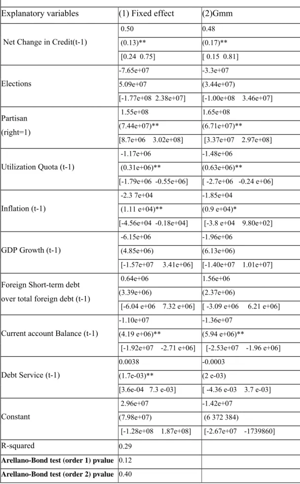
Table 5. New Net Non-Concessional Credit Election influence on IMF
Explanatory variables (1) Fixed effect (2)Gmm
0.50 0.48 (0.13)** (0.17)**
Net Change in Credit(t-1)
[0.24 0.75] [ 0.15 0.81] -7.65e+07 -3.3e+07
5.09e+07 (3.44e+07)
Elections
[-1.77e+08 2.38e+07] [-1.00e+08 3.46e+07] 1.55e+08 1.65e+08
(7.44e+07)** (6.71e+07)**
Partisan (right=1)
[8.7e+06 3.02e+08] [3.37e+07 2.97e+08] -1.17e+06 -1.48e+06
(0.31e+06)** (0.63e+06)**
Utilization Quota (t-1)
[-1.79e+06 -0.55e+06] [ -2.7e+06 -0.24 e+06] -2.3 7e+04 -1.85e+04
(1.11 e+04)** (0.9 e+04)*
Inflation (t-1)
[-4.56e+04 -0.18e+04] [-3.8 e+04 9.80e+02] -6.15e+06 -1.96e+06
(4.85e+06) (6.13e+06)
GDP Growth (t-1)
[-1.57e+07 3.41e+06] [-1.40e+07 1.01e+07] 0.64e+06 1.56e+06
(3.39e+06) (2.37e+06)
Foreign Short-term debt over total foreign debt (t-1)
[-6.04 e+06 7.32 e+06] [ -3.09 e+06 6.21 e+06] -1.10e+07 -1.36e+07
(4.19 e+06)** (5.94 e+06)**
Current account Balance (t-1)
[-1.92e+07 -2.71 e+06] [-2.53e+07 -1.96 e+06] 0.0038 -0.0003 (1.7e-03)** (2 e-03)
Debt Service (t-1)
[3.6e-04 7.3 e-03] [ -4.36 e-03 3.7 e-03] 2.96e+07 -1.42e+07
(7.98e+07) (6 372 384)
Constant
[-1.28e+08 1.87e+08] [-2.67e+07 -1739860]
R-squared 0.29
Arellano-Bond test (order 1) pvalue 0.12 Arellano-Bond test (order 2) pvalue 0.40
The Arellano Bond tests suggest a borderline pattern of autocorrelation of the errors of order one and no error autocorrelation of order two, which is sufficiently coherent with the hypothesis that is behind this estimator. The autoregressive component of the regression is significant and shows a positive and moderately persistent pattern.
The control variables suggested Dreher and Vaubel (2004) are not explicative, with the only exception of the lagged account balance, which is highly significant: the negative coefficient means that an improvement in the value of the account balance is associated with a lowering of the variation of new credit obtained by IMF: this is perfectly in line with the very nature of the Fund, which was born with the mandate of lending to countries with account balance problems.
The behavior of the utilization quota is interesting to take in consideration: the coefficient is negative, highly significant and robust to different specifications: since most of the countries that compose the dataset exhibited in the past problems of high inflation and debt, the negative coefficient could be interpreted as cautiousness from the IMF side in the concession of new debt. An increase in the total liabilities as a percentage of the quota could somehow the Fund nervous and less willing to underwrite new credit lines.
The fund in this case is behaving as a regular financing institution, trying to minimize the risk of default.
However, the real variables of interest are the political ones: in fact, despite the interesting information that is possible to deduce from the partisan variable, election and post-election dummy variables are not significant; the variable post-ele was dropped because in all model specification the p-value associated with the regression was always very high.
The partisan variable coefficient is remarkably significant and positive: If the party in power is right-handed, the net credit will increase of 165 millions of current US dollars. In order to better appreciate the magnitude of the fact, the average of the loan for each country of the dataset for the period 1975-1997 is of 468 millions of current US dollars.
Such a selective behavior regarding the political identity of the recipient country would as well explain partly why the coefficient on election dummy variable is not significant: the relevant matter would be not to enlarge the credit amount but to sponsor governments which display ideological believes closer to the Fund’s vision.
VI. Conclusions
This research investigates the presence of political business cycles in the economic policy instruments and considers the possibility of a reciprocal influence between the IMF and the political incumbents that are seeking reelection.
First, I determine the presence of political business cycle in our dataset, which includes 16 Latin American Countries.
Evidence of PBC was found in the fiscal policy variable, but not in the monetary policy one. The pre-election dummy variable was found to be positive and significant. The result is really robust.
The second part of the question is whether IMF is inducing a problem of Moral Hazard in the recipient country before the election. The policymakers in the recipient country are obviously interested in having a good economic performance before the elections, in order to be reelected. What is to determine is if the presence of IMF credit is helping politicians seeking power or not.
The results are quite interesting: once taken care of the endogeneity of IMF related variables, the increase of new credit given to a country from IMF has as a direct consequence on the amount of budget deficit, that results to be 3 times bigger than during non-election years.
Access to credit seems to exacerbate the willingness of a government to distort the economic cycle for election reasons.
Another result, in line with the public choice literature, is that countries with left-wing parties at the government do tend to have bigger budget deficits that right ones.
The third part of the issue takes the problem dealt in the second part, and reverts the causality: the attention now is on whether the proximity to the election is affecting the behavior of IMF for what concerns the magnitude of the loans.
The most relevant results are the one concerning the behavior of the Utilization Quota and the political variables. For what concerns the utilization quota, in fact, the negative sign of the coefficient suggest that the IMF takes prudential measures to avoid financial risks exactly as any other financial institutions: An increase in the total liabilities due to the Fund decrease, in fact, the quantity of new credit given.
For what concerns the political variables, there is no evidence of exploitation of political business cycle from the part of the IMF.
However there is quite a remarkable effect is the partisan dummy variable coefficient, which is positive and suggests that a consistently bigger amount of credit is accorded to right-hand party governments. This last result suggests the need of stricter and less ambiguous procedures to avoid any political inference from the Fund into recipient countries.
Summing up, the presence of Political Business Cycles is quite evident by looking at the fiscal policy instrument. Governments therefore have the tendency to manipulate the economic cycles to signal their competence. The Presence of Credit given by the IMF seems to worsen the situation, exacerbating the amplitude of the cycle. The IMF, however do not use the delicate moment of election to place more loans. The motivation of personal prestige of the Fund’s bureaucracy does not seem to stand.
Nevertheless, the disparity of treatment in the disbursement of loans on a partisan basis does not seem to follow a strict economic logic.
Bibliography
Alesina, A. Macroeconomic Policy in a Two-Party System as a Repeated Game. Quarterly Journal of Economics 102:651-78 1987
Alesina Roubini Cohen, Political Cycles and the Macroeconomy, The MIT Press, Cambridge 1999
Arellano, Bond, Some Tests of Specification for Panel Data: Monte Carlo Evidence and an Application to Employment Equations, The review of Economic Studies, Vol.58, No.2. April 1991, pp277-297.
Bernhard, Leblang Democratic Institutions and Exchange-rate Commitments International Organization 53, 1, Winter 1999, pp. 71–97 1999 by The IO Foundation and the Massachusetts Institute of Technology
Brenden, Drazen: Political Budget Cycles in New versus Established Democracies, NBER Working Paper no.10539
Clark, Hallemberg: Mobile Capital Domestic Institutions and Electorally Induced Monetary and Fiscal Policy, The American Political Science Review, Vol.94, No. 2, june 2000
Drazen, A.: “The Political Business Cycle After 25 Years. ”NBER Macroeconomics Annual 2000. Cambridge, MA: MIT Press.
Dreher: A public choice perspective of IMF and World Bank lending and conditionality, Public Choice 119: 445–464, 2004.
Dreher, Vaubel: Do IMF and IBRD Cause Moral Hazard and Political Business Cycles? Evidence from Panel Data Open economies review 15: 5–22, 2004, Kluwer Academic Publishers
Ellery Jr., Roberto, Victor Gomes e Adolfo Sachsida 2002. “Business Cycle Fluctuations in Brazil,” Revista Brasileira de Economia 56 (2): 269-308.
Franzese, Robert J. Electoral and Partisan Cycles in Economic Policies and Outcomes Annual Reviews Political Sciences, 2002
Franzese, Robert J. Macroeconomic policies of developed democracies Cambridge University press, Cambridge 2002b
International Monetary Fund (2000) “International Financial Indicators, CD-ROM.” Washington, DC.
International Bank for Reconstruction and Development (2000) “World Development Indicators, CD-ROM.” Washington, DC.
International Financial Institutions Advisory Commission, (IFIAC), Chairman: Allan Meltzer (1999) Report, http://phantomx.gsia.cmu.edu/IFIAC/USMRPTDV. html, 1.9.2000.
Joyce, J : The adoption, implementation and impact of IMF programs: A review of the issues and evidence, Comparative Economic Studies, Vol 46 No.3, September 2004 Persson, T. and G. Tabellini. Macroeconomic Policy, Credibility and Politics. Chur, Switzerland: Harwood Academic Publisher.1990
Rogoff Kenneth, Sibert Anne Elections and Macroeconomic Policy Cycles, The review of Economic Studies, Vol. 55, No. 1(Jan., 1988), 1-16
Thorsten Beck, George Clarke, Alberto Groff, Philip Keefer, and Patrick Walsh, 2001. "New tools in comparative political economy: The Database of Political Institutions." 15:1, 165-176 (September), World Bank Economic Review.
Van Reenen Johnn, Panel Data Estimation of Production Functions, Classroom notes, LSE, 2006, available on the web at:
Annex
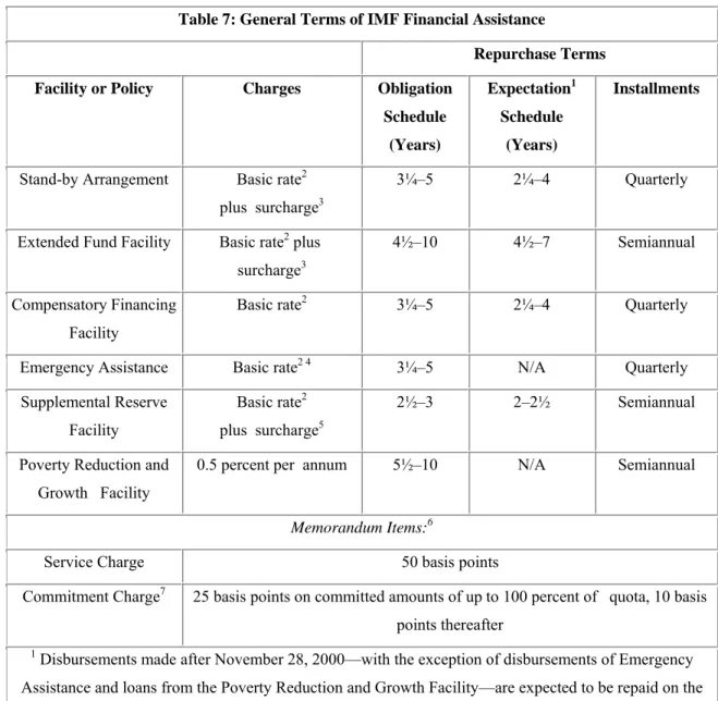
Table 7: General Terms of IMF Financial Assistance
Repurchase Terms
Facility or Policy Charges Obligation
Schedule (Years) Expectation1 Schedule (Years) Installments
Stand-by Arrangement Basic rate2
plus surcharge3
3¼–5 2¼–4 Quarterly Extended Fund Facility Basic rate2 plus
surcharge3
4½–10 4½–7 Semiannual Compensatory Financing
Facility
Basic rate2 3¼–5 2¼–4 Quarterly
Emergency Assistance Basic rate2 4 3¼–5 N/A Quarterly
Supplemental Reserve Facility
Basic rate2
plus surcharge5
2½–3 2–2½ Semiannual Poverty Reduction and
Growth Facility
0.5 percent per annum 5½–10 N/A Semiannual
Memorandum Items:6
Service Charge 50 basis points
Commitment Charge7 25 basis points on committed amounts of up to 100 percent of quota, 10 basis
points thereafter
1 Disbursements made after November 28, 2000—with the exception of disbursements of Emergency
Assistance and loans from the Poverty Reduction and Growth Facility—are expected to be repaid on the expectation schedule. A member not in a position to meet an expected payment can request the Executive
Board to approve an extension to the obligations schedule.
2 The basic rate charge is linked directly to the SDR interest rate by a coefficient that is fixed each financial
year. The basic rate of charge therefore fluctuates with the market rate of the SDR, which is calculated on a weekly basis. The basic rate of charge is adjusted upward for burden sharing to compensate for the overdue
charges of other members (see Box II.9 in Pamphlet 45).
Fund Facility (EFF) is 100 basis points for credit over 200 percent of quota, and 200 basis points for credit over 300 percent of quota. This surcharge is designed to discourage large use of IMF resources.
4 For PRGF-eligible members, the rate of charge may be subsidized to 0.5 percent per annum, subject to the
availability of subsidy resources.
5 The surcharge on the Supplemental Reserve Facility (SRF) is 300-500 basis points, with the initial
surcharge of 300 basis points rising by 50 basis points after one year and each subsequent six months. The surcharge increases over time in order to provide an incentive for repurchases ahead of the obligation
schedule.
6 These charges do not apply to the Poverty Reduction and Growth Facility.
7 Commitment charge does not apply to Compensatory Financing Facility and Emergency Assistance.