On the Hybrid Cramér-Rao Bound and Its Application to Dynamical Phase Estimation

HAL Id: hal-01239443

https://hal-ensta-paris.archives-ouvertes.fr//hal-01239443

Submitted on 7 Dec 2015

HAL is a multi-disciplinary open access

archive for the deposit and dissemination of

sci-entific research documents, whether they are

pub-lished or not. The documents may come from

teaching and research institutions in France or

abroad, or from public or private research centers.

L’archive ouverte pluridisciplinaire HAL, est

destinée au dépôt et à la diffusion de documents

scientifiques de niveau recherche, publiés ou non,

émanant des établissements d’enseignement et de

recherche français ou étrangers, des laboratoires

publics ou privés.

to Dynamical Phase Estimation

Stéphanie Bay, Benoit Geller, Alexandre Renaux, Jean-Pierre Barbot,

Jean-Marc Brossier

To cite this version:

Stéphanie Bay, Benoit Geller, Alexandre Renaux, Jean-Pierre Barbot, Jean-Marc Brossier.

On

the Hybrid Cramér-Rao Bound and Its Application to Dynamical Phase Estimation. IEEE

Sig-nal Processing Letters, Institute of Electrical and Electronics Engineers, 2008, 15, pp.453-456.

�10.1109/LSP.2008.921461�. �hal-01239443�

On the Hybrid Cram´er-Rao bound and its

application to dynamical phase estimation

St´ephanie Bay, Benoit Geller, Alexandre Renaux, Member, IEEE, Jean-Pierre Barbot and Jean-Marc

Brossier

Abstract

This letter deals with the Cram´er-Rao bound for the estimation of a hybrid vector with both random and deterministic parameters. We point out the specificity of the case when the deterministic and the random vectors of parameters are statistically dependent. The relevance of this expression is illustrated by studying a practical phase estimation problem in a non data-aided communication context.

I. INTRODUCTION

A natural problematic when designing an estimator is the evaluation of its performance. Lower bounds on the Mean Square Error (MSE) mainly answer this question and the well known Cram´er-Rao Bound (CRB) is widely used by the signal processing community. Depending on assumptions on the parameters, the CRB has different expressions. When the vector of parameters is assumed to be deterministic, we obtain the standard CRB [1] and when the vector of parameters is assumed to be random with an a priori probability density function (pdf), we obtain the so-called Bayesian CRB [2].

At the end of the eighties, an extension combining both the standard and the Bayesian CRBs has been proposed [3]. Indeed, in some practical scenarios, it is natural to represent the parameter vector by a deterministic part and by a random part. This bound has thus been called the Hybrid CRB (HCRB) and a nice tutorial can be found in [4]. Until now, results available in the literature essentially focussed on the case where the deterministic part and the random part of the parameter vector are assumed to be statistically independent (see, e.g., Eqn. (5) in [3], Eqn. (13)

St´ephanie Bay and Jean-Pierre Barbot are with the Ecole Normale Sup´erieure de Cachan, SATIE Laboratory, 61, avenue du President Wilson 94235 Cachan, France. (e-mail: {bay,barbot}@satie.ens-cachan.fr)

Benoit Geller is with Ecole Nationale Sup´erieure des Techniques Avanc´ees, Laboratory of Electronics and Computer Engineering (LEI), 32, Boulevard Victor 75015 Paris, France. (e-mail: geller@ensta.fr)

Alexandre Renaux is with University Paris-Sud 11, Laboratory of Signals and Systems, Sup´elec, 3 rue Joliot-Curie, 91192 Gif-sur-Yvette cedex, France. (e-mail: renaux@lss.supelec.fr)

Jean-Marc Brossier is with Grenoble Institute of Technology, GIPSA Laboratory, 961 rue de la Houille Blanche Domaine universitaire - BP 46 38402 Saint Martin d’H`eres cedex, France. (e-mail: jean-marc.brossier@gipsa-lab.inpg.fr)

This work was supported in part by the French ANR (Agence Nationale de la Recherche), LURGA project and by the European network of excellence NEWCOM++.

in [4] and Eqn. (13) in [5]). To the best of our knowledge, a closed-form expression of the HCRB with a statistical dependence between the deterministic and the random parameters has never been reported in the literature. The goal of this paper is then twofold. First, in Section II, we remind the structure of the HCRB and we point out the specificity of the case when the deterministic part and the random part of the parameter vector are statistically dependent. Second, in Section III, motivated by this analysis we give a closed-form expression of the proposed bound in the practical case of a dynamical phase subject to a linear drift in a non data-aided communication context.

II. THE HYBRIDCRAMER´ -RAO BOUND

A. Background

Let µ =¡µT r µTd

¢T

∈ Rn _{be the parameter vector that we have to estimate. This vector is split into two}

sub-vectors µ_d and µ_rwhere µ_d is assumed to be a (n − m) × 1 deterministic vector and µ_ris assumed to be a m × 1 random vector with an a priori pdf p (µ_r). The true value of µd will be denoted µ?d. We consider ˆµ(y) as an

estimator of µ where y is the observation vector. The HCRB satisfies the following inequality on the MSE

Ey,µr|µ?d · (ˆµ(y) − µ) (ˆµ(y) − µ)T ¯ ¯ ¯ µ? d ¸ ≥ H−1(µ?d) , (1)

where H (µ?_d) ∈ Rn×n _{is the so-called Hybrid Information Matrix (HIM) defined as [3]}

H (µ?d) = Ey,µr|µ?d h − ∆µµ log p( y, µr| µd) ¯ ¯ µ? d i , (2) where£∆ν η ¤ k,l= ∂2 ∂[η]k∂[ν]l.

When the deterministic and the random parts of the parameter vector are assumed to be independent, and after some algebraic manipulations, the HIM can be rewritten as (see [4], Eqn. (18))

H (µ? d) = Eµr[F(µ ? d, µr)] +   Eµr £ −∆µr µrlog p (µr) ¤ 0m×(n−m) 0(n−m)×m 0(n−m)×(n−m)   , (3) where F(µ?d, µr) = Ey|µ? d,µr h − ∆µµ log p( y| µd, µr) ¯ ¯ µ? d i . (4)

With this aforementioned structure, it is straightforward to reobtain the standard and the Bayesian CRBs. Indeed, if µ = µ_d, we have H−1_(µ? d) = µ Ey|µ? d · − ∆µd µ_d log p( y| µd) ¯ ¯ ¯ µ? d ¸¶−1 , (5)

which is the standard CRB, and, if µ = µ_r, we have

H−1₌³_E y,µr h −∆µr µ_r log p( y| µr) i + Eµr £ −∆µr µrlog p (µr) ¤´−1 , (6)

B. Extension when µ_r and µ_d are statistically dependent

We now assume a possible statistical dependence between µ_rand µ_d. In other words, µ_r is now assumed to be a m × 1 random vector with an a priori pdf p ( µ_r| µ?

d) 6= p (µr).

Based on the HIM definition given by Eqn. (2) and expending the log-likelihood as log p¡y, µr|µ?d

¢

= log p (y|µ? d, µr)+

log p (µr|µ?d), we obtain the following HIM

H (µ? d) = Eµr|µ?d[F(µ ? d, µr)] + Eµr|µd? h − ∆µ µlog p (µr|µd) ¯ ¯ µ? d i , (7)

where F(µ?_d, µ_r) is given by Eqn. (4).

In order to explicitly show the modification in comparison with the HIM given by Eqn. (3), H (µ?_d) can be rewritten as follows H (µ?d) = Eµ_r|µ? d[F(µ ? d, µr)] + Eµ_r|µ? d     −∆ µ_r µrlog p (µr|µ ? d) − ∆ µ_r µdlog p (µr|µd) ¯ ¯ µ? d ³ − ∆µr µ_dlog p (µr|µd) ¯ ¯ µ? d ´T − ∆µd µ_dlog p (µr|µd) ¯ ¯ µ? d     . (8)

Obviously, if we assume p ( µ_r| µd) = p (µr) in this expression, we straightforwardly reobtain Eqn. (3).

Based on this structure, one now has to prove that there is still an inequality, i.e., a lower bound on the MSE,

Ey,µr|µ?d · (ˆµ(y) − µ) (ˆµ(y) − µ)T ¯ ¯ ¯ µ? d ¸ ≥ H−1(µ?d) , (9)

when H (µ?_d) is given by Eqn. (8).

Proof: Following the idea of [4] to prove the inequality (1), one defines a vector h such that

h =   ∇µlog p (y, µr|µd)|µ? d ˆ µ (y) − µ|_µ? d   , (10) where ∇µ= ³ ∂ ∂[µ]₁ · · · ∂[µ]∂_n ´T .

Consequently, the non-negative definite matrix G (µ?_d) = Ey,µ_r|µ? d

£

h hT¤ _{can be decomposed as the following}

block matrix G (µ?d) =   H (µ?d) L (µ?d) LT_(µ? d) R (µ?d)   , (11)

where R (µ?_d) is the covariance matrix of ˆµ (y), i.e.,

R (µ? d) = Ey,µr|µ?d · (ˆµ(y) − µ) (ˆµ(y) − µ)T ¯ ¯ ¯ µ? d ¸ , (12)

and, where L (µ?_d) is given by

L (µ? d) = Ey,µr|µ?d · ∇µlog p (y, µr|µd)|µ? d ³ ˆ µ (y) − µ|_µ? d ´T¸ . (13)

Since G (µ?_d) ≥ 0, its Schur complement satisfies

R (µ?

d) ≥ LT(µ?d) H−1(µ?d) L (µ?d) . (14)

It is straightforward to show that, for an unbiased estimator w.r.t. the pdf p ( y, µ_r| µ?_d), L (µ?_d) = In×n.

Consequently, the inequality (9) is proved and H−1(µ?

III. HCRBFOR A DYNAMICAL PHASE ESTIMATION PROBLEM

In [6], we have proposed a closed-form expression of the Bayesian CRB for the estimation of the phase offset for a BPSK transmission in a non data-aided context. In this section, we extend these previous results by providing a closed-form expression of the HCRB for the estimation of the phase offset and also of the linear drift. In this more realistic scenario, we show that we have to take into account the statistical dependence between the parameters and, consequently, the HCRB given by Eqn. (3) is not adapted to this problem.

A. Observation and state models

We consider a linearly modulated signal, obtained by applying to a square-root Nyquist transmit filter an unknown symbol sequence a = (a1· · · aK)T taken from a unit energy BPSK constellation. The signal is transmitted over

an additive white Gaussian noise channel. The output signal is sampled at the symbol rate which yields to the observations

yk = akejθk+ nk with k = 1 . . . K, (15)

where {nk} is a sequence of i.i.d., circular, zero mean complex Gaussian noise variables with variance σ2n. We

consider that the system operates in a non Data-Aided synchronization mode, i.e., the transmitted symbols are i.i.d. with Pr(ak= ±1) = 1₂.

In practice, several sources of distortions affect the phase. An efficient model representing these effects is the so-called Brownian phase with a linear drift widely studied in the literature (see, e.g., [7] [8] [9]). This model takes into account a constant frequency shift between the oscillators of the transmitter and of the receiver, the uncertainities due to clocks, and, the jitters of oscillators. The Brownian phase model with a linear drift is given as follows

θk = θk−1+ ξ + wk with k = 2 . . . K, (16)

where, for any index k, {θk} is the sequence of phases to be estimated, ξ represents the deterministic unknown

linear drift with true value ξ?, and where {wk} is an i.i.d. sequence of centered Gaussian random variables with

known variance σ2_w.

The parameter vector of interest is then made up of both random and deterministic parameters µ =¡µT_r µ_d¢T where µ_r= θ = (θ1· · · θK)T and µd = ξ. Moreover, from Eqn. (16), it is clear that p ( θ| ξ?) 6= p (θ).

B. Derivation of the HCRB

For notational convenience, we drop the dependence of the different matrices on µ?_d = ξ? in the remainder of this paper. From Eqn. (8), the HIM H can be rewritten into a block matrix H =

  H11 h12 h21 H22  , where,              H11= Ey,θ|ξ? h − ∆θ θlog p (y|θ, ξ) ¯ ¯ ξ? i + Eθ|ξ? £ −∆θ θlog p (θ|ξ?) ¤ , h12= hT21= Ey,θ|ξ? · − ∆ξ_θlog p (y|θ, ξ) ¯ ¯ ¯ ξ? ¸ + Eθ|ξ? · − ∆ξ_θlog p (θ|ξ) ¯ ¯ ¯ ξ? ¸ , H22= Ey,θ|ξ? · − ∆ξ_ξlog p (y|θ, ξ) ¯ ¯ ¯ ξ? ¸ + Eθ|ξ? · − ∆ξ_ξlog p (θ|ξ) ¯ ¯ ¯ ξ? ¸ . (17)

These blocks only depend on the log-likelihoods log p ( y| θ, ξ?) and log p ( θ| ξ?). Let us set y = (y1· · · yK)T

and assume that the initial phase θ1 does not depend on ξ, i.e., p (θ1|ξ?) = p (θ1). Using Eqn. (15) and (16), i.e.,

the Gaussian nature of the noise and the equiprobability of the symbols, one has

  

log p (y|θ, ξ?) =PK_k=1³− log¡πσ2

n ¢ −1+kyk_σ2 k2 n + log ³ cosh³ 2 σ2 n< © yke−jθk ª´´´ ,

log p (θ|ξ?) = log p (θ1) + (K − 1) log

³ 1 √ 2πσw ´ −PK_k=2(θk−θk−1−ξ?)2 2σ2 w . (18)

• Expression of H11: assuming that we have no prior knowledge, i.e., Eθ1

h ∆θ1

θ1log p(θ1)

i

= 0, it is shown in

[6] (due to the order one Markov structure exhibited by Eqn. (16)) that H11 takes the following tridiagonal

structure H11= b             A + 1 1 0 · · · 0 1 A 1 . .. ... 0 . .. . .. . .. 0 .. . . .. 1 A 1 0 · · · 0 1 A + 1             , (19)

where b = −1/σ2_w, and, where A = −σ2_wJD− 2 with JD= Ey,θ|ξ?

h

−∆θk

θklog p (yk|θk, ξ

?₎i

.

• Expression of h12: since, from Eqn. (18), log p (y|θ, ξ?) is independent of ξ?, ∆ξ_θlog p (y|θ, ξ)

¯ ¯ ¯ ξ? = 0. Consequently, h12= Eθ|ξ? · − ∆ξ_θlog p (θ|ξ) ¯ ¯ ¯ ξ? ¸ . (20)

Using the state model, we have

           ∆θ1 ξ log p (θ|ξ) ¯ ¯ ¯ ξ?= − 1 σ2 w, ∆θK ξ log p (θ|ξ) ¯ ¯ ¯ ξ?= 1 σ2 w, ∆θk ξ log p (θ|ξ) ¯ ¯ ¯ ξ?= 0 for k ∈ {2, . . . , K − 1} . (21)

Applying the expectation operator Eθ|ξ?[.], we obtain

h12= ³ 1 σ2 w 01×K−2 − 1 σ2 w ´T . (22)

• Expression of H22: since, from Eqn. (18), log p (y|θ, ξ?) is independent of ξ?, ∆ξξlog p (y|θ, ξ)

¯ ¯ ¯ ξ? = 0. Consequently, H22= Eθ|ξ? · − ∆ξ_ξlog p (θ|ξ) ¯ ¯ ¯ ξ? ¸ = K − 1 σ2 w . (23)

• Expression of the HCRB: we now give the expression of H−1 which bounds the MSE. Thanks to the block-matrix inversion formula, we have

H−1 ₌   H−111 + VK −_λ1H−111h12 −1 λhT12H−111 λ1   , (24) where λ = K−1_σ2 w − h T 12H−111h12and VK = 1_λH−111h12hT12H−111.

We start to compute λ corresponding to the inverse of the minimal bound on the MSE of ξ. Due to the particular structure of matrices H11 and h12 (Eqn. (19) and (22)), we obtain

λ = K − 1 σ2 w − 2 σ4 w ³£ H−1 11 ¤ 1,1− £ H−1 11 ¤ 1,K ´ . (25)

From Eqn. (19), thanks to the cofactor expression in the matrix inversion formula we have for any index k,

£ H−111

¤

1,k= b k−1

|H11|(dK−k+ b dK−k−1) where dk is the determinant of the following k × k matrix Dk

Dk= b             A 1 0 · · · 0 1 A 1 . .. ... 0 . .. . .. . .. 0 .. . . .. 1 A 1 0 · · · 0 1 A             . (26)

The sequence {dk} satisfies the following recursive equation dk = A b dk−1− b2dk−2 with d0 = 1 and

d1= bA. dk can thus be written as dk= ρ1(r1)k+ ρ2(r2)k where r1, r2, ρ1 and ρ2 are given by

   r1= b₂ ¡ A +√A2_{− 4}¢_{, r} 2= b₂ ¡ A −√A2_{− 4}¢_, ρ1= √ A2_−4+A 2√A2₋₄ , ρ2= √ A2_−4−A 2√A2₋₄ . (27) Consequently, £ H−1 11 ¤ 1,k= bk−1 |H11| ¡ ρ₁rK−k−1 1 (r1+ b) + ρ2rK−k−12 (r2+ b) ¢ , (28) and λ = K − 1 σ2 w − 2 σ4 w|H11| ¡ ρ1rK−21 (r1+ b) + ρ2rK−22 (r2+ b) − bK−1 ¢ . (29)

From the definition of VK, we have

[VK]_k,k= 1 λσ4 w ³£ H−1 11 ¤ 1,k− £ H−1 11 ¤ 1,K+1−k ´2 . (30)

Using Eqn. (24), (28), and (30), we obtain, for any index k, the analytical expression of the HCRB diagonal elements £ H−1¤_k,k= 1 |H11| · ρ21(b + r1)2rK−31 + ρ22(b + r2)2r2K−3− b2 A − 2(r k−2 1 rK−k−12 + rK−k−11 rk−22 ) ¸ + 1 λ σ4 w|H11|2 h bk−1³_ρ 1 (r1)K−k−1(b + r1) + ρ2 (r2)K−k−1(b + r2) ´ + bK−k³_ρ 1 (r1)k−2(b + r1) + ρ2 (r2)k−2(b + r2) ´i2 . (31)

Remark: Note that, if Eqn. (3) was used instead of Eqn. (8), the HIM would not be invertible.

C. Simulation results

We now illustrate the behavior of the HCRB versus the Signal-to-Noise Ratio (SNR) defined by _σ12

n. We consider

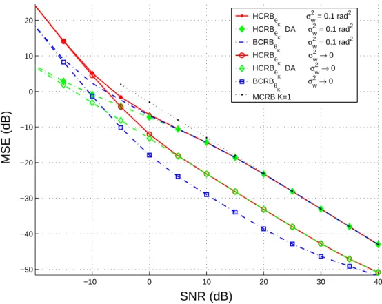
a block of K = 40 BPSK transmitted symbols. For two distinct phase-noise variances (σ2_w = 0.1 rad2 and σ2_w→

0 rad2), Figure 1 superimposes on one side the HCRB (see Eqn. (31)), the Data-Aided HCRB

³

JD=_σ22

n

´

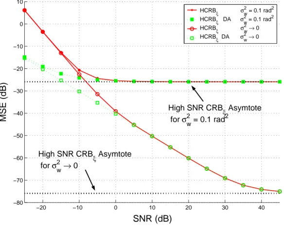
the BCRB (see Eqn. (21) in [6]) on θK. For the same scenario, Figure 2 superimposes on one side the HCRB (see

Eqn. (25)) and the Data-Aided HCRB on ξ.

• At high SNR, we first notice that HCRBξ converges to its horizontal asymptote given by σ

2

w

K−1 which is the

standard CRB when θ is assumed to be known. The observation noise compared to the phase noise is then not significant enough to disturb the estimation of ξ; consequently HCRBξ depends only on the phase noise

and on the number of observations. Concerning the bounds on θK, HCRBθk and BCRBθk both have the same

asymptote given by σ2n

2 which is the Modified CRB (MCRB) for one observation (see [10]). It means that,

at high SNR, the observation yK is self-sufficient to estimate θK and the error on ξ does not disturb the

performance on θK. Moreover, the HCRB logically tends to the Data-Aided HCRB.

• For median SNR, HCRBθK and HCRBξ leave their respective asymptote. HCRBθK is still lower bounded by

the BCRB and upper bounded by the high-SNR asymptote. This stems from the fact that taking into account a block of observations instead of one observation necessarily improves the performance. However, for large

σ2

wvalues (e.g., σ2w= 0.1 rad2), HCRBθK stays close to the MCRB because the correlation between the phase

offsets θk is less significant than the information brought by the observation yK. Moreover, when σ2w tends

to 0, HCRBθK is above the BCRB because performance is now limited by the accuracy on the parameter ξ.

• At low SNR, nk is preponderant compared to wk. Both HCRBξ and HCRBθK do not depend on σ 2

w: the

lack of knowledge on ξ directly affects the estimation on θK. As expected, the knowledge of the symbols

(Data-Aided HCRB) leads to a better estimation of θ and ξ.

IV. CONCLUSION

In this paper, we have studied the hybrid Cram´er-Rao bound when the random and the deterministic parts of the parameter vector are statistically dependent. We have applied this bound in order to evaluate the performance of a dynamical phase estimator where the linear drift is unknown in a non data-aided context. In particular, we have illustrated the effect of this unknown linear drift on the phase estimation performance.

REFERENCES

[1] H. Cram´er, Mathematical Methods of Statistics, ser. Princeton Mathematics. New-York: Princeton University Press, Sept. 1946, vol. 9. [2] H. L. Van Trees, Detection, Estimation and Modulation Theory. New-York, NY, USA: John Wiley & Sons, 1968, vol. 1.

[3] Y. Rockah and P. Schultheiss, “Array shape calibration using sources in unknown locations–part I: Far-field sources,” IEEE Transactions

on Acoustics, Speech, and Signal Processing, vol. 35, no. 3, pp. 286–299, Mar. 1987.

[4] H. Messer, “The hybrid Cram´er-Rao lower bound – from practice to theory,” in Proc. of IEEE Workshop on Sensor Array and Multi-channel

Processing (SAM), Waltham, MA, USA, July 2006, pp. 304–307.

[5] A. M. Guarnieri and S. Tebaldini, “Hybrid Cram´er-Rao bounds for crustal displacement field estimators in SAR interferometry,” IEEE

Signal Processing Letters, vol. 14, no. 12, pp. 1012–1015, Dec. 2007.

[6] S. Bay, C. Herzet, J.-M. Brossier, J.-P. Barbot, and B. Geller, “Analytic and asymptotic analysis of Bayesian Cram´er-Rao bound for dynamical phase offset estimation,” IEEE Transactions on Signal Processing, vol. 56, no. 1, pp. 61–70, Jan. 2008.

[7] P.-O. Amblard, J.-M. Brossier, and E. Moisan, “Phase tracking: what do we gain from optimality? Particle filtering versus phase-locked loops,” Signal Processing, vol. 83, no. 1, pp. 151–167, Jan. 2003.

−10 0 10 20 30 40 −50 −40 −30 −20 −10 0 10 20

SNR (dB)

MSE (dB)

HCRB_θ K σ w 2 = 0.1 rad2 HCRB θ K DA σ w 2 = 0.1 rad2 BCRB θ K σ w 2 = 0.1 rad2 HCRB θ_K σw 2_→ 0 HCRB θ_K DA σw 2_→ 0 BCRB_θ K σ w 2_→ 0 MCRB K=1

Fig. 1. Bounds on θK versus the SNR (K = 40 observations, σ2w= 0.1 rad2, and σ2w → 0 rad2, JD evaluated over 108 Monte-Carlo

trials).

[9] A. Demir, A. Mehrotra, and J. Roychowdhury, “Phase noise in oscillators: a unifying theory and numerical methods for characterization,”

IEEE Trans. on Circuits and Systems, vol. 47, pp. 655–674, May 2000.

[10] M. Moeneclaey, “On the true and the modified Cram´er-Rao bounds for the estimation of a scalar parameter in the presence of nuisance parameters,” IEEE Transactions on Communications, vol. 46, no. 11, pp. 1536–1544, Nov. 1998.

−20 −10 0 10 20 30 40 −80 −70 −60 −50 −40 −30 −20 −10 0 10

SNR (dB)

MSE (dB)

HCRB_ξ σ w 2 _{= 0.1 rad}2 HCRB_ξ DA σ w 2 _{= 0.1 rad}2 HCRB_ξ σ w 2_{→ 0} HCRB_ξ DA σ w 2_{→ 0}

High SNR CRB

_ξ

Asymtote

for

σ

2 w

→

0

High SNR CRB

_ξ

Asymtote

for

σ

2 w

= 0.1 rad

2