Open Archive TOULOUSE Archive Ouverte (OATAO)
OATAO is an open access repository that collects the work of Toulouse researchers and
makes it freely available over the web where possible.
This is an author-deposited version published in :
http://oatao.univ-toulouse.fr/
Eprints ID : 10464
To cite this version : Narcy, Marine and De malmazet, Eric and Colin,
Catherine. Flow boiling in straight heated tubes under microgravity
conditions. (2013) In: 8th International Conference on Multiphase Flow - ICMF
2013, 26 May 2013 - 31 May 2013 (Jeju, Korea, Republic Of).
Any correspondance concerning this service should be sent to the repository
administrator:
[email protected]
81h International Conference on Multiphase Flow
ICMF 2013, Jeju, Korea, May 26-31, 2013
Flow Boiling in Straight Heated Tubes
Under Microgravity Conditions
Marine Narcy1, Erik De Malmazee, Catherine Colin1
1
/nstitut de Mécanique des Fluides de Toulouse, Université de Toulouse, France
Keywords: flow boiling, two-phase flow, microgravity, heat transfer, wall friction
Abstract
Forced convective boiling experiments with HFE-7000 were conducted in earth gravity and under microgravity conditions. The experiment mainly consists in the study of a boiling flow (liquid-vapour flow) through a 6 mm diameter sapphire tube uniformly heated by an ITO coating. Measurements of pressure drops (on an adiabatic section), void fraction and wall and liquid temperatures are provided. High-speed movies of the flow are also taken. The data were collected in normal gravity and during a series of parabolic trajectories flown in an airplane. Flow visualizations, temperature, pressure and void fraction measurements are analysed to obtain flow pattern, heat transfer, film thickness and wall friction data.
Introduction
Two-phase thermal systems are broadly used in various industrial applications and engineering fields: flow boiling heat transfer is common in power plants ( energy production or conversion ... ), transport of cryogenie liquids and other chemical or petrochemical processes. Thus, the understanding of boiling mechanisms is of importance for accidentai off-design situations. These systems take advantage of latent heat transportation, which generally enables a good efficiency in heat exchanges.
For that reason, two-phase thermal management systems are considered as extremely beneficiai for space applications. lndeed, in satellites or space-platforms, the major thermal problem is currently to remove the vast heat amount generated by deviees from the inside into the space, in order to ensure suitable environmental and working conditions. Moreover, the growing interest for space applications such as communication satellites and the increasing power requirements of on-board deviees lead to an urgent need of sophisticated management systems capable to deal with larger heat loads. Since the heat transfer capacity associated with phase change is typically large and with a relatively little increase in temperature, this solution could mean decreased size and weight of thermal systems.
But boiling is a complex phenomenon which combines heat and mass transfers, hydrodynamics and interfacial phenomena. Furthermore, gravity consequently affects the fluid dynamics and may lead to unpredictable performances of thermal management systems. It is thus necessary to perform experiments directly in (near) weightless environments. Besides the ISS, microgravity conditions can be simulated by means of a drop-tower, a parabolic flight in aircraft or a sounding-rocket.
Although flow boiling is of great interest for space
applications under microgravity conditions, few experiments have been conducted in low gravity. These experiments provided a partial understanding of the boiling phenomena and have been mostly performed for engineering purposes. Moreover, flow boiling heat transfer experiments in microgravity (referred to as ll-g) are subject to severe restriction in the test apparatus, do not last long and offer few opportunities to repeat measurements for repeatability, which could explain the lack of data and of coherence between existing measurements. Nevertheless, several two-phase flow (gas-liquid flow and boiling flow) experiments have been conducted in the past forty years and enabled to gather data about flow patterns, pressure drops, and heat transfers including critical heat flux and void fraction in thermohydraulic systems. Previous state of the art and data can be found in the papers of Colin et al. (1996), McQuillen et al. (1998), Ohta (2003), and Celata and Zummo (2009).
Several studies have been carried out under microgravity conditions in order to classify adiabatic two-phase flows by various patterns through observation and visualizations of the flow. V arious patterns have been identified at different superficial velocities of liquid j1 and gas jv, patterns which are also encountered in boiling flows: bubbly flow, slug flow and annular flow. Transitions flows have been studied too: the determination of these transitions is of importance because the wall friction and wall heat transfer are very sensitive to the flow pattern. Colin et al. (1991) and Dukler et al. (1988) drew a map based on void fraction transition criteria to predict patterns in liquid-gas flows. These patterns were also observed in boiling convective for heat transfer smaller than the critical heat flux by Ohta (2003), Lebaigue et al. (1998), Reinarts (1993) and more recently by Celata and Zummo (2009). A general flow pattern map
for bubbly and slug flows based on the value of the Ohnesorge number was proposed by Colin et al. (1996) for air-water flow and also boiling refrigerants. The transition between slug and annular flow has also been investigated by several authors, who proposed criteria based on transition void fraction value (Dukler at al., 1988), critical value of a vapour Weber number (Zhao and Rezkallah, 1993), balance between gas inertia and surface tension (Reinarts, 1993; Zhao and Hu, 2000).
The estimation of void-fraction or averaged gas velocity is a key-point for the calculation of wall and interfacial frictions.
It has been shown that the mean gas velocity Uv
=
jv/a is well predicted by a drift flux model U0 = C0• j for bubblyand slug flow (Colin et al., 1991), j being the mixture velocity and Co a coefficient depending on the local void fraction and gas velocity distributions. Few experimental data of film thickness were provided, but only for gas-liquid annular flows (Bousman, 1995; de Jong and Gabriel, 2003 ... ).
Regarding the measurements of the wall shear stress, most of the studies performed under microgravity conditions concern gas-liquid flow without phase change (Bousman and McQuillen, 1994; Zhao and Rezkallah, 1995; Colin et al., 1996; Choi et al., 2002). Sorne results also exist for liquid-vapour flow (Chen et al., 1991), but only in an adiabatic test section. Recently, Awad and Musychka (2010) and Fang and Xu (2012) proposed modified correlations of Lockhart and Martinelli and found a good agreement with the experimental data. Very few studies reported data on the interfacial shear stress in annular flow (Dukler et al., 1988). This can be explained by the fact that such a measurement is based on pressure drop and liquid film thickness measurements which remain a difficult task.
Few researches on flow boiling heat transfer have been conducted, mainly because of the restrictive experimental conditions. Lui et al. (1994) carried out heat transfer experiments in subcooled flow boiling with R113 through a tubular tests section (12 mm internai diameter, 914.4 mm length). Heat transfer coefficients were approximately 5 to 20 % higher in microgravity, generally increasing with higher qualities, which was believed to be caused by the greater movement of vapour bubbles on the heater surface. Ohta et al. (1995, 1997, and 2003) studied flow boiling of FC-72 and R113 in vertical transparent tubes ( 4,6 and 8 mm internai diameters ), internally coated with a gold film, both on ground and during parabolic flight campaigns, and for a future experiment in the ISS. Authors examined various patterns and the influence of gravity levels on heat transfer coefficients for two-phase forced-convection heat transfer regime. It was noticed that the influence of gravity is not evident for high mass fluxes (G superior to 250 kg.s-1.m-2). This observation was also made by Baltis, Celata and Zummo (2009) who performed subcooled flow boiling experiments with FC-72 in Pyrex tubes (2, 4 and 6 mm internai diameters). It was shown that the heat transfer coefficient decreases by up to 30-40% in microgravity in comparison with terrestrial gravity and that an increase of mass or heat flux seems to reduce the influence of gravity. A new technique for the measurement of heat transfer distributions has also been developed: Kim and al. (2012)
81h International Conference on Multiphase Flow
ICMF 2013, Jeju, Korea, May 26-31, 2013
used an IR camera to determine the temperature distribution within a multilayer consisting of a silicon substrate coated with a thin insulator. They have not quantified the difference between microgravity and normal gravity yet. W ork has still to be done to confirm and give coherence to the previous results of the literature on flow boiling and to compare the data sets obtained by the different authors.
Objectives
In this work, the authors intend to collect, analyse and compare flow boiling data in normal gravity or under microgravity conditions, thanks to a parabolic flight campaign. The working fluid is the HFE-7000 which circulates in a heated test section made up of a 6 mm inner diameter sapphire tube with a conductive transparent ITO coating. Flow patterns, void fraction, wall friction and heat transfer are studied.
This paper presents the results of the measurement campaigns within three major sections. The first section describes the experimental apparatus and the measurement techniques and accuracy. The data reduction to obtain the mass quality, gas velocity, heat transfer coefficient and wall shear stress is described in a second section. Finally the experimental results obtained in J..L-g and 1-g experiments are presented and discussed.
Nomenclature Cp heat capacity (J.K-1.kg-1) D tube diameter (rn) g gravitational acceleration (m.s -2 ) G mass flux (kg.m-2.s-1 )
h heat transfer coefficient (W.m -2.K-1) l!.h1,v enthalpy ofvaporization (J.kg -1)
j volumetrie flux or superficial velocity (m.s-1)
Nu Nusselt number (-) p pressure (bar) R radius (rn) q heat flux (W.m -2) T temperature (0C) x vapour quality (-) !!.T subcooling (0C) Greek letters a void fraction (-) e permittivity (-) p density (m3.kg-1) 't shear stress (Pa)
Subscripts e environment internai in inlet conditions 1 liquid phase 0 outer
out outlet conditions sat saturation conditions sub subcooled conditions
v vapour phase
Experimental test setup
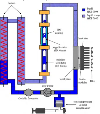
The experimental set-up mainly consists of a hydraulic loop which is represented in Figure 1. In this pressurized circuit, the working fluid is the refrigerant 1-methoxyheptafluoro-propane (C3F70CH3), which will be referred as HFE-7000.
It is first pumped at liquid state by a gear pump while the liquid flow rate is measured by a Coriolis flowmeter. The fluid is heated to its boiling point and partially vaporized in two seriai heaters. Then it enters a stainless steel tube just upstream the test section. In the test section, the HFE-7000 is further vaporized in a 6 mm diameter sapphire tube heated through an outside ITO coating (upward flow). The fluid is then condensed and cooled down 1 0°C below its saturation
temperature into four cold plates including Peltier modules and fans before it enters the pump again. The pressure is adjusted in the circuit via a volume compensator, whose bellow can be pressurized by air.
heaters • liquid HFE 7000 ~ liquid + vapor HFE 7000 heat sink fans
constant pressure .,...___ volume
compensa tor
Figure 1: Schematic of the experimental apparatus. The HFE-7000 has been chosen as working fluid for safety reasons and because of its low saturation temperature at atmospheric pressure (34°C at 1 bar) and its low latent beat of vaporization. In the circuit, the HFE-7000 may be in a liquid or a liquid-vapour state depending on the portion of the hydraulic circuit, but it is never in a pure vapour state. The loop pressure is set from 1 to 2 bars and the fluid circulates with mass fluxes G between 50 and 1200 kg.s -1.m -2 . A wide range of flow boiling regimes is studied, from subcooled flow boiling to saturated flow boiling, by adjusting the power input of the heaters (vapour mass qualities up to 0.9) and the power of the ITO coating (wall beat flux up to 45 000 W.m -2).
The test section is represented in Figure 2. It mainly consists of a 20 cm long sapphire tube with a 6 mm inner diameter and a 1 mm thickness. The outer surface is almost totally coated with ITO, an electrical conductive and transparent
81h International Conference on Multiphase Flow ICMF 2013, Jeju, Korea, May 26-31,2013
coating which enables a uniformly heating by Joule effect and a visual display of the flow.
dllfemltial thmooooupk 200mm
1
sappbîrerube ~,
____ _ PIIOOprobesFigure 2: Schematic of the test section.
V arious measurement instruments pro vide experimental data for the calculation of pressure drops and beat transfer: • adiabatic section: two differentiai pressure transducers measure the pressure drop along an adiabatic section at the outlet of the test section.
• test section:
- pressure: two absolute pressure sensors are used to calculate the saturation temperature at the inlet and outlet of the sapphire tube. No differentiai pressure measurement is performed on this section.
- temperature: type K thermocouples are used to measure the flow temperature at the test section inlet and outlet. Two type T thermocouples are also used to measure the temperature difference between a hot junction and a cold junction located at the inlet and outlet of the test section, respectively. This differentiai thermocouple allows a very accurate measurement of the liquid temperature evolution along the test section. Ptl 00 probes measure the ambient temperature and the temperature of the externat surface of the sapphire tube at four different positions
- visualization: a high speed camera provides movies of the flow through the ITO coating.
- void fraction: specifie void fraction probes were designed and built at IMFT to provide accurate data of the volume fraction of the vapour phase. These sensors measure the capacitance between two copper electrodes which depends on the fraction of liquid and vapour in the considered volume. One of them is represented in Figure 3. Liquid HFE-7000 and Teflon roads are used to mimic the annular flow configuration for the calibration.
copper electrodes liquid HFE7000 PEEK section vapor HFE7000 , _ , 6mm
Figure 3: Schematic of a void fraction probes. Experiments were conducted both on ground and under microgravity conditions. A weightless situation is simulated during a parabolic flight campaign which consists of three flights with around 31 parabolas per flight. Each parabola
provides up to 22 seconds of microgravity with a gravity level smaller than 3.10-2 g.
During the on-ground measurement campaign, relevant parabolas were reproduced in order to compare data obtained in normal gravity and under microgravity conditions. A series of parametric runs bas also been conducted to complete the database.
Data reduction
Hereafter, the calculations of beat transfer coefficients, vapour quality and wall friction are presented. These values are deduced from the measurements of wall and liquid temperatures, beat flux, pressure drop and void fraction by
using mass, momentum and enthalpy balance equations.
> Calculation of the beat transfer coefficient
A cross-section of the
sapphire tube is
represented in Figure 4. Tiw and Tow are the inner and outer temperatures of the
sapphire tube wall,
respectively. T eoo is the
external temperature far
from the tube ("at
infmity") and T;00 is the
fluid bulk temperature in Figure 4: Notations.
the tube far from the wall.
Tin and Tout are the liquid bulk temperatures at the inlet and outlet of the sapphire tube. The inner and outer radii of the sapphire tube are denoted by Ri and Ro, respectively. The sapphire thermal conductivity is denoted by k. The ITO coating on the external surface of the test section provides a beat flux qow· The beat flux qiw delivered to the fluid is considered as equal to qow corrected by the radii ratio RJRi. The beat transfer between the internai flow and the internai wall of the sapphire tube is characterized by the beat transfer coefficient hi. The beat transfer between the environment and the external wall of the sa pp hire tube (thermal losses) is characterized by the beat transfer coefficient he.
Following hypotheses are made: 1) Temperature profiles are axisymmetric. 2) The axial conduction can be neglected. 3) The beat transfer by radiation and the beat transfer with the environment can be neglected.
An energy balance in steady state between the inner and outer walls of the tube leads to expressions (l) and (2).
ln
(~~).Ro
Tow- Tiw
=
[qw- he. (Tow- Teoo)]. k (1)Ro
hi. (Tiw- Tioo)
= -.
[qow- he. (Tow- Teoo)] (2) RiThe temperature evolution between Tin and Tout is
considered as linear or parabolic, which enables to calculate
1;00 • If thermal losses are neglected ( on-ground experiments confirm this hypothesis ), the beat transfer coefficient hi can be expressed in function of qiw. Tow and Tiw
> Calculation of vapour quali!Y
The vapour quality can be calculated by using the total enthalpy conservation equation in steady state. qiw is the wall beat flux delivered to the fluid by Joule effect through
81h International Conference on Multiphase Flow ICMF 2013, Jeju, Korea, May 26-31,2013
the ITO coating, and Di is the inner diameter of the sapphire tube.
• for saturated boiling regimes: if T1 is the liquid temperature, T1
=
Tsat• which leads to the expression (3). The evolution of the mass quality can be directly calculated with the wall beat flux and the vapour quality at the inlet of the test section is considered as equal to the vapour quality at the outlet of the heaters.4.qiw dx
---v:-=
G. dhl,v· dz (3)1
Considering that the wall beat flux is constant, a linear evolution of vapour quality is observed. The vapour quality at the inlet of the test section is deduced from an energy balance in the preheaters. In this case, the vapour quality calculated with the total enthalpy conservation equation is equal to the classical thermodynamic vapour quality. • for subcooled boiling regimes, we have T1
< Tsat
and the vapour temperature is assumed to be equal to the saturation temperature. The enthalpy balance equation for the mixture can be written:4. qiw d ( )
- - =
-d Pv· a. Uv. hv sat+
PI· (1 - a). UL. hLDi z ·
d ( G. [x. hv,sat
+
)
=
dz (1-x). (hl,sat+
Cpl. (Tl- Tsat))l
(
4)where h1 is the liquid enthalpy and hv,sat and h1,sat are the vapour and liquid enthalpies at saturation temperature, respective! y.
The wall beat flux leads to an increase of the total enthalpy of the mixture, both by phase change and by increasing the liquid temperature: 4.qiw ( )
ax
---v:-=
G. dhtv+
Cp1. (Tsat-T1) •az
1aT
1 +G. Cp1• (1 -x).az
(5) For the experiments in subcooled boiling, a single-phase flow is observed at the inlet of the test section. Indeed, a 22 cm long stainless steel tube enables to condensate potential bubbles coming from the two seriai heaters. Then the inlet quality is 0 and equation (5) leads to the expression of x through a global balance:4. Lheated· qiw- G. Di. Cpl. (Tout- Tin)
~~= G. Di. d tv- Cpi(Tout- Tin)
[h'
]
(6)where dhJ.v
=
dhl,v+
Cpl. (Tsat - T1) (7)For both cases, the fluid temperature is measured at the inlet and outlet of the test section and the temperature evolution between these two points is considered as linear.
The calculation of the vapour quality in subcooled boiling is tricky because of the order of magnitude of x and of measurement uncertainties. W e can define measurement errors dqw on the measured wall beat flux and dT1 on the
measured liquid temperature. Measurement errors on mass
flux G, and geometrical and physical properties are
neglected. By considering Equation (5), the error lu on a low vapour quality can be expressed:
4. dqw Lheated Cpl dx ~
-
.
-·c
Ah +Ah .dT1 (8) D1 • Ll l,v Ll l,v 103 16.10-2 13.102 d - 4 - -+ - -
210-1 x - . 6.10-3 • 8. 102.14. 104 14. 104 • • dx oc 2.10-3The error on the vapour quality is 2.1
o-
3, which is the orderof magnitude of x itself. This error was confmned by an analysis of flow videos by comparing the mean hubble velocity measured from the images and those calculated using the void fraction and the quality values.
> Calculation of the wall friction
The two differentiai pressure transducers measure the pressure drop llP along an adiabatic section at the outlet of the test section, which enables to write the momentum balance equation in steady state without the acceleration term depending of the vapour quality:
dP 4
dz
=v·
"rw-g. [Pv· a+ PL· (1-a)] (9)By integrating Equation (9) between the inlet and the outlet of the test section, the wall friction can be expressed according to the pressure difference along the adiabatic section and the void fraction:
_ -~ ioutlet â.P - D. "rw.dz inlet
i
outlet+
g. (Pv· a(z)+
PL· (1 - a(z))). dz lnlet (10) llP is measured by the differentialtransducers (there is no va pour in transmissions lines) and a is measured at the inlet and outlet of the test section by two void fraction probes. In J.L-g, the last term of equation (10) can be neglected. On ground, in vertical flow, the last term is dominant, thus the accuracy on the wall shear stress measurement is directly linked to the accuracy on the void fraction measurement itself.Measurements for single-phase flows in normal gravity have enabled to validate the measurement technics and calculation protocols by confronting the data to standard correlations.
> Pressure drops validation
For the wall friction coefficient
lw
in single-phase flow in normal gravity, the Blasius correlation based on the global Reynolds number Re is used:fw = 0,0791. Re-0•25 (11)
Figure 5 shows the measurements obtained with the two
differentiai transducers in 1-g for single-phase flows with various mass fluxes and the Blasius' correlation with error bars at+lO% and-10%.
2 0.0120 0.0060 oldt oumber Re
...
.
...
.... ....
~....
~
....
.._ fwl (measured) + fw2 (meuurcd) --Blasius +10"/o.
....
....
20000...
6
..
...
....
•
81h International Conference on Multiphase Flow
ICMF 2013, Jeju, Korea, May 26-31, 2013
FigureS: Wall friction coefficient in single-phase flow
> Heat transfer coefficient validation
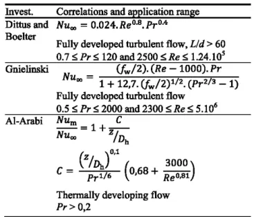
For a fully developed turbulent single-phase flow, the Nüsse1t number Nu" can be calculated with the Dittus and Boelter's correlation (Table 1) and the Gnielinski's correlation (Table 1 ), based on the Reynolds number Re and
the Prandtl number Pr. The wall friction coefficient
lw
is calculated with the Blasius' correlation. z is the distance between the probe and the inlet of the heated section andDn
is the hydraulic diameter which is equal to the inner diameter Di.Invest. Correlations and application range Dittus and Nu00
=
0.024.Re0·8.Pr0.4
Boetter
Gnielinski
Al-Arabi
Fully developed turbulent flow, Lld > 60 0.7 '5. Pr '5. 120 and 2500 :'5. Re '5. 1.24.105
lfw/2).
(Re - 1000). PrNu.,
=
1+
12,7. (fw/2)112 • (Pr213 - 1) Fully developed turbulent flow0.5 '5. Pr '5. 2000 and 2300 '5. Re '5. 5.106
( tl
c
=
z~~
16
(o,68+
:~~~
1
)
Thermally developing flow
Pr> 0,2
Table 1: Nüsselt correlations for full y developed and thermally developing flows in smooth and circular ducts.
Nüsselt numbers corresponding to the four Pt1 00 probes located on the outer surface of the sa pp hire tube for various mass fluxes in single-phase flows are calculated and compare to the Gnielinski's correlation. The deviation from the correlation is in inverse proportion to the distance between the temperature sensors (1, 2, 3 or 4) and the inlet of the heated section; hence the hypothesis of a thermally developed flow in the sapphire tube is not satisfied.
Whenever the flow is thermally developing, a local heat transfer coefficient corresponding to a mean Nüsselt number
NUm is measured. This number must be corrected according to the distance between the measurement point and the inlet of the heated section in order to calculate the fully developed flow Nüsselt number Nuœ and to compare it with
correlations. Figure 6 shows the measurements corrected with Al-Arabi's correlation (Table 1) and compared to the Gnielinski's formula .
The experimental data corrected according to the sensor position meet the Gnielinski's correlation with a maximal error of ±17%. The error depends of the mass flux (that varies the thermal entrance length) and of the probe position. The precision between measurements and correlations is satisfying for the whole set of experiments in single-phase flow. It also confirms the weak impact of externat thermal heat losses on the measurements.
~
...
..
,1:> 8=
=
.J5
"' "'·=
z
80 70 60 50 40 30 20 10 0 0 • Nul • Nu2 0 Nu3 <> Nu4 - - - Gnielinski - - - Dittus-Boelter 20% 1000 2000 3000 4000 5000 6000 7000 8000 Reynolds number ReFigure 6: Measured Nüsselt number with correction.
Results and Discussion
Experimental results about flow patterns, wall friction and
heat transfer coefficients are presented. Preliminary data concerning the evolution of the liquid film thickness in
annular flow are also plotted.
Flow patterns
The high speed camera has enabled to visualize flow
patterns for various mass fluxes G, vapour qualities x at the
inlet of the test section and heat fluxes qow through the ITO
coating. Three main flow patterns have been observed in
both normal gravity and microgravity conditions: annular flow, slug flow and bubby flow were identified on the videos. Another flow pattern is also referred in the literature as slug/annular transition.
(a)
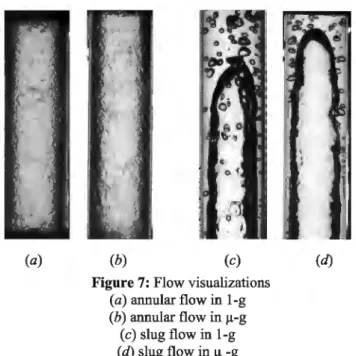
(b) (c)Figure 7: Flow visualizations
(a) annular flow in 1-g
( b) annular flow in JJ.-g (c) slug flow in 1-g (d) slug flow in J.l. -g
(d)
Figure 7 shows annular flow and slug flow with nucleated
boiling in 1-g and JJ.-g, and Figure 8 shows a comparison
between bubbly flows in 1-g and JJ.-g for the same
parameters (G, x and qow). Bubbly flows correspond to
subcooled regimes (T1 < Tsat). The impact of gravity level on
the bubbles size and shape can be seen in the videos for mass fluxes lower than 400 kg.s-1.m-2: under microgravity
conditions, bubbles are larger than in normal gravity and are not deformed by the gravity field. The larger hubble size in
ath International Conference on Multiphase Flow
ICMF 2013, Jeju, Korea, May 26-31,2013
microgravity can be explained by both the larger hubble diameter at detachment and the higher rate of coalescence. A vapour quality increase leads through a coalescence phenomenon to slug flow which alternates between long
Taylor bubbles and liquid plugs that can be aerated by small
bubbles. Coalescence of long Taylor bubbles indicates the transition to annular flows which almost always correspond to saturated regimes (11 = T831). The precision of the flow
parameters setting and the camera spatial resolution do not
enable to see clearly differences between 1-g and JJ.-g in the
videos for annular flows.
(a) (b) (c)
Figure 8: Flow visualizations bubbly flows, ~Tsub = 12 °C, q = 2 W.cm-2
G = 540 kg.s-1.m-2 (a) in 1-g, (b) in JJ.-g
G = 220 kg.s-1.m-2 (c) in 1-g, (d) in JJ.-g
(d)
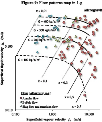
Figures 9 and 10 show flow patterns maps for the experiments performed in normal gravity and under
microgravity conditions, respectively. Regimes are
indicated according to the superficial vapour and liquid
velocities, and isocurves for G and x are added.
x= 0,01 Normal gravity ~---o-•• / G = 400 kg/sim' ~~a~~~ ... LJ .~--- - - '"V'-'...rl : / G = 300 kg/s/m2 ---..-u.r
-..
.::0----~-~-
i
/ G = 200 kg/s/m2!' ..
.. 0.10//::=
100 kg/s/m2 ....
...., - - ~-<r-z--
t:.'!f::_~....
·
...
...
9
..
'
...
.... ....
x= 0,1 ~patterns jo 1.:& : 0Bubbly Flow.C. Transition and slug Flow
.C. Transition annular 0 Annular Flow x= 0,3 ! \ x=0,5 ... \ 0 x= 0,7 0 0.01 +---~---~--0.10 1.00 10.00
Figure 9: Flow patterns map in 1-g x ~ 0,01 M.lcrogravlty
~~-
_
<:tf)
--.<>-
<!:
-
/:,
0 0 ,/ G~
400kg/s/~Z
0~
'Q'O
... - - - -
-<>~---
,0 0 Q)O ,./ G~
300kg/s/mZ
~
/~
0/"'-
-4-
&
...t:>-
4::.
~
....
0 6. ..8
/ G~
~
kg/s/mi> 6.6..
~~
0 . :' o ~ ~ 0.100l
1
.. 6. .• 6./
~0
:' <> ... 0 0 0,/
<>
./
o
t
rl.l ~--- - / 0 0 - - · oo G = 100 kg/s/mZ : - ..., • 0 :' 0...
..~
§)
,./
0..
..
,~,.s
... .....
~
x~ 0,1 .E_1m potterm tn.~ : 0 Annular flow <>Bubbly t1ow..
/ \...
'
x~ 0,3 :' ' :'/
,
..
..
..
'
x~
0,5 /,./q
âSlug flow and trmlsition flow x ~0,7
O.DIO + r _ ; _ . . , . . . .
-0.100 1.000 10.000
Superficial vapour velocity iv (mis)
Figure 10: Flow patterns map in 1-1-g
Because of the uncertainty about the calculation of the vapour quality, experimental points for x inferior to 0.01 are not shown. Figure 1 0 presents relevant parabolas performed during the fust and second flight campaigns for mass fluxes up to 400 kg.s·'.m-2• Indeed, a preliminary data reduction just after the fust measurement campaign bas underlined the fact that gravity effect was not clearly quantifiable for mass fluxes G superior to 400 kg.s·'.m-2• Therefore, no experiments and parametric runs were performed in 1-g and ).L-g for G > 400 kg.s·'.m-2 afterwards.
In normal gravity, the transition between bubbly and annular flow occurs very fast for low mass fluxes, typically at x
around 0.1. For higher mass flux, this transition seems to last within a larger x range and sorne subcooled annular flows can be observed, but these regimes were not further investigated. Bubbly and slug flows evolve toward annular flow earlier in microgravity (transition around x = 0.08 -0.09 for Iower mass fluxes) than in normal gravity (transition around
x
= 0.1) because of the more important coalescence phenomenon.Film thic:kness
The data set used to study the film thickness contains runs whose points are in both annular and transitional flows (near the slug-to-annular region). The calculations are made by assuming that ali the liquid is included in the liquid film surrounding the vapour core (the droplets entrainment phenomenon is neglected). With this hypothesis, the film thickness is directly obtained with the void fraction data, as a time averaged value.
Results are shown in Figure 11 for both microgravity and normal gravity conditions. The liquid film thickness ~ is
~lo~d as a function of the vapour ~uality for two different liqu1d mass fluxes (G = 400 kg.s·'.m· and 200 kg.s-'.m-2).
B1h International Conference on Multiphase Flow
ICMF 2013, Jeju, Korea, May 26-31, 2013
0.50 0.40
j
-0.30 ~J
0.20i
~ 0.10 Film th!cknBH; ~G = 200 kg/sim1- 1-g•
a
= 200 kglsim1 -O-g AG= 400 kg/sim1 - 1-g AG= 400 kg/sim1 -0-g 0.00 +--r----.----r--""""T""--r---r---r---. 0.000 0.100 0.200 0.300 0.400 0.500 0.600 0.700 0.800 Vapour quality x [-]Figure 11: Liquid ftlm thickness in 1-g and ~-g
As can be seen from Figure 11, changing the vapour quality has a significant influence on the liquid film thickness which decreases as x increases through a non-linear process, both in ).L-g and 1-g (an asymptote can be observed as x increases to high qualities). Changing the liquid mass flux has less effect on ô, even if an increase of the mass flux G
leads to an increase of the film thickness at a constant vapour quality. This is consistent with the fact that annular flow is dominated by the increasing effect of liquid and gas inertial forces compared to the gravity forces.
Moreover, it can be seen that for given vapour quality and mass flux, a change in the gravity level leads to important changes in the film thickness. Even if the difference between 1-g and jl-g depends on the mass flux, there is a clear tendency towards a thinner liquid film in microgravity. On ground, the gravity force tends to drive the liquid film downwards, leading to a larger film thickness.
Wall friction
In microgravity, the gravity term of Equation (9) can be neglected. Therefore, the wall friction can be directly deduced from the pressure drop measurement.
During the fust campaign, the V alidyne transducers were located on the heated test section. Preliminary reduction using Martinelli' s relationship for the determination of a. bas shown that the inertia term represents up to 20% of the pressure drop and cannot be neglected in the global balance. By taking this consideration into account, the differentiai pressure measurement was moved to an adiabatic, which enables to neglect the inertia term.
Figure 12 and Figure 13 represent the experimental two-phase frictional multiplier cDw in normal gravity and microgravity respectively, compared to the one predicted by the Lockhart and Martinelli's correlation (1949). The experimental cDw is calculated from the wall shear stress measurements, and plotted versus the Martinelli's parameter
X given in Equation 11.
X=f.J_
~
fwliv.
Pv fwv (11) 2 (c
1) <I>Lo = 1+ +
-X X2 (12)1 Laminar 1 turbulent 1 12 1 40 35
i
30..
25t
~
20 E! :i 15•
.cl 10l
5 0 0.01 0.1 Prepure dnmt la 1-g:- - Lock:hart & Martinelli (tt) Lock:hart & Martinelli (lt)
0 Sulx:ooled data 0 Saturated data
10
M1111inelli's plll'ameter X
Figure 12: Pressure drops in normal gravity compared to Lockhart and Martinelli's correlation
35 ~ 30 9 2s
..
l2o
1
15 :i.a
10l
5 Pn:ynre dnmt I.D p-g: - Lock:hart & Martinelli (tt)Lockhart. & Martinelli (lt)
0 Saturated Data 0 Sulx:ooled data
0 L---~~~
----0.01 0.1 10
Mardnelli't piU'ameter X
Figure 12: Pressure drops in microgravity compared to Lockhart and Martinelli' s correlation
The significant error on the superficial vapour velocity for low vapour qualities (subcooled data) leads to an underestimation of the associated two-phase multiplier for the bubbly flows. On the other hand, the saturated data (corresponding to annular flows) are in very good agreement with the Lockhart and Martinelli's correlation in 1-g. The same trend can be observed with the IJ--g data that fit the correlation with a 5% mean deviation for the annular regime data and 27% mean deviation for the bubbly regime data.
Beat transfer coefficients
Heat transfer coefficients in 1-g and in IJ--g for saturated boiling regimes and subcooled boiling regimes are presented in Figures 13, 14 and 15.
The precision of the calculation of hi (also denoted h) is directly linked to the measurement accuracy of qfi'N and of temperatures (wall and liquid bulk temperatures) and to the chosen evolution of the temperature in the sapphire tube between Tm and Tout· By using a linear evolution of the temperature in the heated section and by considering uncertainties Aqw and AT on the heat flux and temperatures, respectively, heat transfer coefficients can be calculated with an error bar at ±14%.
6000
B1h International Conference on Multiphase Flow
ICMF 2013, Jeju, Korea, May 26-31, 2013
Beat trulfer coeflldeat in 1-g
~
~
5000 D D .c:]
..
c.. ..
'!!
Ill
b!
4000 3000 2000 D ~--- --!:;. - - - -!:;. ... .,.-
...
~···-~.
.,.
..,.
...
--~---~ !:;. •••••• -., ···:;... • 0 . · · · · - 0 0..
x;;·-1000 -1--~-~--r----r----r----r---~----. 0.05 0.15 0.25 0.35 0.45 0.55 0.65 0.75 0.85 Vapour qulity x [-] Kandlikar - G = 200 kg/s/m' Chen -G = 200 kg/s/zril. • G=200 kg/111m2 -tg C G~400 kg/111m2 -tg Kandlikar-G=300 qjs/zril. 0 G = 100 kg/s/nr- lg 6 G = 300 kgfs/nr - lgFigure 13: Heat transfer coefficients in 1-g for saturated boiling flows (annular flows) according to the vapour
quality for qi = 2 W .cm '"2 and for various mass fluxes Results about heat transfers are difficult to summarized because the coefficient hi and the different correlations depends on various parameters such as the vapour quality, mass flux, heat flux or gravity level.
Figure 13 shows heat transfer coefficients according to the vapour quality for a wall heat flux qi= 2 W.cm'"2 and mass
"1 "2 d G 400 k "1 "2
fluxes between G = 100 kg.s .m an = g.s .m , for saturated boiling regimes.
Measurements in normal gravity are compared with two boiling heat transfer correlations: Chen's correlation (1966) and Kandlikar's correlation (1989) which brings into play the boiling number and a coefficient linked to the Martinelli's parameter. At a given mass flux, the evolution of hi on ground is the expected one: the heat transfer coefficient increases with the vapour quality at fixed heat flux, and increases with heat flux at fixed vapour quality. The heat transfer coefficients also increase with G on the chosen mass fluxes range. Measurements in normal gravity fit the empirical correlations ( calculated for given q and G)
with a mean deviation from Kandlikar's correlation that is around 16%.
At G = 200 kg.s ·'.m-2, the effect of gravity lev el on boiling heat transfer is more quantifiable than for higher mass rates (results from the frrst parabolic flight campaign have shown that at G = 500 kg.s-1.m-2, the mean difference on h; between 1-g and IJ--g is ±3.5%). For that reason, Figure 14 shows experimental heat transfer coefficients in microgravi!?' for mass fluxes G ranging from 100 kg.s-1.m-2to 300 kg.s· .m-2•
Heat transfer data are given for a heat flux q; = 2 W .cm-z and compared with Chen and Kandlikar's correlations.
6000 ~
g
5000 ~ ..::=
..
4000~
~ 3000 y 0.15 0.25 0.35 0.45 0.55 0.65 0.75 0.85 Vapour quality x 1-1 Kandlikar - G = 200 kg/m2/s 0 G=IOOkg/m2/s- Og Kandlikar G=300 kg/m2/s•
G=200 kg/m2/s-Og Chen - G = 200 kg/m2/s 1:;. G=300 kg/m2/s-OgFigure 14: Heat transfer coefficients in f-1.-g for saturated
boiling flows (annular flows) according to the vapour quality for qi= 2 W.cm·2 and for various mass fluxes
As can be seen from Figure 14, it seems that the beat transfer coefficients are lower in microgravity than in normal gravity for low vapour qualities (x < 0.2 at G = 200 kg.s·'.m-2). For these qualities, Kandlikar's correlation overestimates the f-1.-g beat transfer coefficient. On the other band, the beat transfer coefficients are higher in f-1.-g than in 1-g for high vapour qualities (x > 0.2 at G = 200 kg.s·'.m-2) and Kandlikar's correlation underestimates h in this case. The experiments performed in subcooled boiling flows tend to confirm this trend, as can be seen from Figure 15.
3500
h (microgravity) > h (normal gravity)
~
3000 h 1-g=hO-g~
-10% 2500 t>.ll=
1 -25% ..:: 2000=
..
·o
s
..
1500 0 y...
1000 ~"'
=
..
.l: 500 -;..
=
h (microgravity) < h (normal gravity)0
700 1200 1700 2200 2700 3200
Beat transfer coefficient h-lg [W/m1/K)
Figure 15: Heat transfer coefficients in 1-g and f-1.-g for subcooled boiling flows (bubbly flows) for various beat fluxes and mass fluxes between 100 and 400 kg.s·'.m-2 The subcooled data points (bubbly flows data in Figure 15) correspond to vapour qualities inferior to 20% (x< 0.2). For ali these points (whatever the beat flux, mass flux or vapour quality is ), the beat transfer coefficient is lower in microgravity than in normal gravity (by 20% on average). These results are consistent with the one in saturated flow
81h International Conference on Multiphase Flow ICMF 2013, Jeju, Korea, May 26-31,2013
regimes. This trend bas to be confirmed by additional experiments. In bubbly flow, the hubble slip velocity is close to zero in microgravity, whereas it is significant in vertical flow on ground. This relative velocity induces a distorsion of the velocity profile near the wall and an increase of the velocity gradient and turbulence level in the liquid flow (Colin et al., 2012). This effect is also responsible for an increase of the wall friction in bubbly flow and may explain the larger beat transfer coefficient in normal gravity.
Conclusions
This paper presents the results of flow boiling experiments performed under microgravity conditions during two parabolic flight campaigns and compared to parametric runs conducted on ground. The objective was to collect beat transfer, void fraction and wall friction data along a heated test section consisting of a 6 mm inner diameter heated sapphire tube, using HFE-7000 as working fluid.
Special attention was paid to the calculation of the vapour quality in arder to characterize properly the subcooled boiling regimes, but it remains difficult to investigate flows with very low superficial vapour velocities .
Annular flow, slug flow and bubbly flow have been observed in videos according to the vapour quality and the mass fluxes. The results show that the gravity level bas little impact on the flow for mass fluxes superior to 400 kg.s-1.m-2 whatever the flow pattern is. That is the reason why lower mass fluxes were investigated in this article.
The transition between slug and annular flow seems to occur at lower qualities in microgravity.
Experimental pressure drops data fit the Lockhart and Martinelli's correlation with a good agreement both in normal gravity and microgravity.
On-ground beat transfer values are in good agreement with classical correlations of the literature. However, significant discrepancies with these correlations are found in microgravity. Flow boiling beat transfer at low mass fluxes under microgravity conditions can be either increased for high vapour qualities or reduced by up to 30% for vapour qualities inferior to 20%, which is consistent with the film thickness data that show that the liquid film is thinner under microgravity conditions .
Additional experiments at lower mass fluxes should be conducted in arder to validate this trend. Another parabolic flight campaign will be the opportunity to perform new experiments in microgravity. Future test matrix plans to conduct runs at lower mass fluxes by adapting the hydraulic loop and to improve the accuracy on the temperature measurement for the calculation of the vapour quality. Further data processing may enable to access the interfacial friction and new beat transfer madel.
Acknowledgements
The authors would like to acknowledge the French and
European Space Agencies CNES and ESA for having funded
this study and the parabolic flight campaigns. The Fondation de Recherche pour l'Aéronautique et l'Espace is also thanked for its financial support.
References
Al-Arabi, M., Turbulent Heat Transfer in the Entrance Region of a Tube, Heat Transfer Eng., (3): 76-83 (1982) Awad M.M., Muzychka Y.S., Review and modeling of two-phase frictional pressure gradient at microgravity conditions, Fluid Enginnering Division Summer Meeting ASME, Montreal, August 2010 (2010)
Baltis, C.H.M., Celata, G.P., Zummo, G., Multiphase Flow Heat Transfer in Microgravity, Internai communication (2009)
Blasius, H., Das Àhnlichkeitsgesetz bei Reibungsvorgangen in Flüssigkeiten, Forschg. Arb. Ing.-Wes., (131): Berlin (1913)
Celata, G.P., Zummo, G., Flow Boiling Heat Transfer in Microgravity: Recent Progress, Multiphase Science and Technology, Vol. 21, No. 3, pp. 187-212 (2009)
Chen, I.Y., Downing, R.S., Keshock, E., Al-Sharif, M., Measurements and correlation of two-phase pressure drop under microgravity conditions, Journal ofThermophysics, 5, 514-523 (1991)
Colin, C., Fabre, J., Mc Quillen, J., Bubble and slug flow at microgravity conditions: state of knowledge and open questions, Chem. Engng. Com., 141-142, 155-173 (1996) Colin C., Fabre, J., Dukler, A.E., Gas-Liquid flow at microgravity conditions-!: Dispersed bubble and slug flow, Int. J. Multiphase Flow, 17, 533-544, 1991 (1991)
Colin, C., Fabre, J., Gas-liquid pipe flow under microgravity conditions: influence of tube diameter on flow patterns and pressure drops, Adv. Space Res., 16, pp. (7)137-(7)142 (1995)
Colin, C., Fabre, J., Kamp A., Turbulent bubbly flow in a pipe under gravity and microgravity conditions, J. Fluid Mech., vol. 711, pp. 469-515 (2012)
Fang, X., Zhang, H., Xu, Y., Su, X., Evaluation of using two-phase frictional pressure drop correlations for normal gravity to microgravity and reduced gravity, Adv. Space Res., 49, 351-364 (2012)
Gnielinski, V., New Equations for Heat and Mass Transfer in Turbulent Pipe and Channel Flow, !nt. Chem. Eng., (16): 359-368 (1976)
Jong, P., Gabriel, K.S, A preliminary study of two-phase flow at microgravity: experimental data of film thickness, !nt. J. Multiphase Flow, 29, 1203-1220 (2003)
Kim, T.H., Kommer, E., Dessiatoun, S., Kim, J., Measurement of two-phase flow and beat transfer parameters using infrared thermometry, !nt. J. Multiphase Flow, 40 (2012) 56--67 (2012)
Lebaigue, 0., Bouzou, N., Colin, C., Results from the Cyrène experiment: convective boiling and condensation of
81h International Conference on Multiphase Flow
ICMF 2013, Jeju, Korea, May 26-31, 2013 ammonia in microgravity, 281
h Int. Conf. on Environmental
Systems, Danvers, Massachusetts (1998)
Lockhart, R. W., Martinelli, R. C., Proposed Correlation of Data for Isothermal Two-Phase, Two-Component Flow in Pipes, Chemical Engineering Progress Symposium Series, 45 (1), pp. 39-48 (1949)
Lui, R.K., Kawaji, M., and Ogushi, T., An Experimental Investigation of Subcooled Flow Boiling Heat Transfer Under Microgravity Conditions, lOth International Heat Transfer Conference -Brighton, Vol. 7, pp. 497-502 (1994) Ma, Y., Chung, J.N., A Study of Bubble Dynamics in Reduced Gravity Forced-Convection Boiling, Int. J. Heat Mass Transfer, 44, 399-415 (2001)
Nebuloni, S. And Thome, J.R., Numerical modeling of laminar annular film condensation for different channel shapes, Int. J. Heat and Mass Transfer, 53, 2615-2627 (2010)
Ohta, H., Experiments on Microgravity Boiling Heat Transfer by Using Transparent Heaters, Nuclear Engineering and Design, Vol. 175, pp. 167-180 (1997) Ohta, H., Fujiyama, H., Inoue, K., Yamada, Y., Ishikura, and S., Yoshida, S., Microgravity Flow Boiling in a Transparent Tube, Proc. 4th ASME-JSME Thermal Engineering Joint Conf., Lahina, Hawaii, USA, pp. 547-554 (1995)
Ohta, H., Microgravity beat transfer in flow boiling, Advances in heat transfer, Vol37, 1-76 (2003)
Reinarts, T. R., Adiabatic two phase flow regime data and mode ling for zero and reduced (horizontal flow) acceleration fields, PhD dissertation, Univ. of Texas A&M (1993)
Rohsenow, W.M., Hartnett, J.P., Cho, Y.I., Forced convection, internai flow in ducts », Handbook of Heat Transfer, Third Edition, 5.2 (1998)
Saito, M., Yamaoka, N., Miyazaki, K., Kinoshita, M., and Abe, Y., Boiling Two-Phase Flow Under Microgravity, Nuclear Engineering and Design, Vol. 146, pp. 451-461 (1994)
Zhao, L., Rezkallah, K.S., Gas liquid flow patterns at microgravity conditions, !nt. J. Multiphase Flow, 19, 751-763 (1993)
Zhao, L., Rezkallah, K.S., Pressure drop in Gas-Liquid flow at microgravity conditions Gas liquid flow patterns at microgravity conditions, !nt. J. Multiphase Flow, 21, 837-849 (1995)
Zhao, L., Hu,W.R., Slug to annular flow transition of microgravity two-phase flow, International Journal of Multiphase Flow 26, 1295-1304 (2000)