Aeroelastic Limit Cycle Oscillations Mitigation Using
Linear and Nonlinear Tuned Mass Dampers
Edouard VERSTRAELEN
Department of Aerospace and Mechanical engineering
University of Li`ege
A thesis submitted for the degree of
Doctor of Philosophy
Members of the Examination Committee GILET, Tristan - President - Professor at University of Li`ege
DIMITRIADIS, Grigorios - Supervisor - Professor at University of Li`ege KERSCHEN, Ga¨etan - Supervisor - Professor at University of Li`ege RAVEH, Daniella - Professor at Technion Israel Instritute of Technology DE TROYER, Tim - Professor at Vrije Universiteit Brussel
Abstract
Flutter is a destructive aeroelastic phenomenon occurring on flexible aeronau-tical structures because of an energy exchange between two or more of the system’s vibration modes and an airflow. In some rare cases, limit cycle oscil-lations (LCOs) related to flutter are observed because of nonlinearities, which might require aircraft redesign or flight envelope limitations. One way of sup-pressing such LCOs could be using Linear and Nonlinear Tuned Vibration Absorbers ((N)LTVAs), which are widely used in civil engineering but have to date received very little attention in the aerospace community.
The objectives of this thesis are the understanding of nonlinear aeroelastic phenomena and the investigation and demonstration of the beneficial effects of such absorbers for flutter and LCO suppression. Two nonlinear aeroelastic systems featuring smooth (continuously hardening) and non-smooth (freeplay) nonlinearities are investigated by means of mathematical models and wind tunnel experiments.
An increase in flutter speed of up to 35% is observed on the former system, both in the wind tunnel and using the model, however, a very precise tuning of the absorber’s natural frequency is required. On the other hand, a negli-gible increase in LCO onset speed is observed on the latter system although a reduction in LCO amplitude of up to 60% is achieved in a given airspeed range, using a nonlinear absorber whose nonlinearity mimics that of the aeroe-lastic apparatus. The effect of linear and nonlinear vibration absorbers on the shape of the limit cycle branches of aeroelastic systems is described in detail and it is shown that such devices can change the nature of bifurcations from supercritical to subcritical and vice versa and can even cause the appearance of isolated solution branches. Therefore, extreme care must be taken when designing and implementing LTVAs and NLTVAs, as their effectiveness in in-creasing the linear flutter speed can be compromised by the change in the nature of the bifurcation. Furthermore, it is shown that a LTVA can not only delay classical flutter but also delay/suppress stall flutter.
Acknowledgements
Even though this thesis only bears my name, it wouldn’t have seen the light of the day without the support of many people whom I would like to express my gratitude to, for their support but also for for making this journey enjoyable and enriching.
First, I would like to thank all the people without whom nothing would have been possible: my advisors, Gaetan Kerschen and Greg Dimitriadis for their trust, guidance, support and availability, the European Union for the funding (ERC Starting Grant NoVib 307265), and the members of the jury for taking the time to review this work.
Then, I would like to thank my friends and colleagues Marco, Thibaut, Vin-cent, Samir, Thomas and all the others, for all the technical (or not) discussions that provided (hopefully) good ideas, a good working atmosphere, a proper understanding of the plot of Game of Thrones and amazing ”B” strategies. I spent quite a bit of time fiddling with bolts, bearings and aluminium bits and I would like to thank Mathieu and Antonio for their help and their advice. Twenty seventeen has been a rough year and I would like to thank all those who contributed in making it brighter.
I would also like to thank the Colettes for watering my parents’ plants on that 8th of August and for all the fond memories that arose from that day, in Russia, in Durham, in Blindeff, in the Swabs, in Angleur, and everywhere else. Last but not least, I would like to thank my family and all my friends for everything. I wish I had something cool to tell them but unfortunately I do not right now. Sorry folks.
« Attention
cette th`ese n’est pas
une th`ese sur
le cyclimse »
Contents
Contents ix
1 Introduction 1
1.1 Aeroelastic problems throughout history . . . 1
1.2 State of the art in nonlinear aeroelasticity . . . 4
1.2.1 Linear flutter . . . 5
1.2.2 Nonlinear aeroelasticity . . . 5
1.3 Vibration mitigation techniques . . . 15
1.3.1 Active control . . . 15
1.3.2 Passive control via structural aircraft modifications . . . 16
1.3.3 Passive control via dynamic absorbers . . . 17
1.4 Objectives of the thesis . . . 24
2 Design, analysis and modelling of a pitch and flap wing 25 2.1 Introduction . . . 25
2.2 Experimental setup . . . 26
2.3 Wind-off identification . . . 30
2.3.1 Linear identification . . . 30
2.3.2 Nonlinear identification . . . 32
2.4 Pre-critical aeroelastic investigation . . . 36
2.5 Post-critical aeroelastic investigation . . . 38
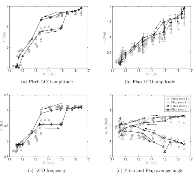
2.5.1 Bifurcation diagrams . . . 38
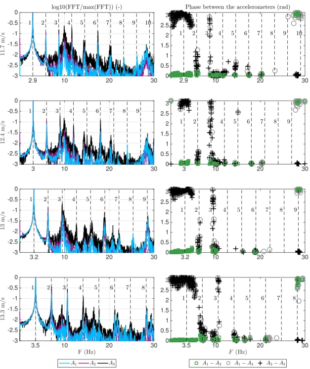
2.5.2 Waterfall plots . . . 40
2.5.3 Airflow separation visualisation using wool tufts . . . 43
2.5.4 Experimental results summary . . . 46
2.6 Mathematical model . . . 47
2.7 Mathematical model validation . . . 48
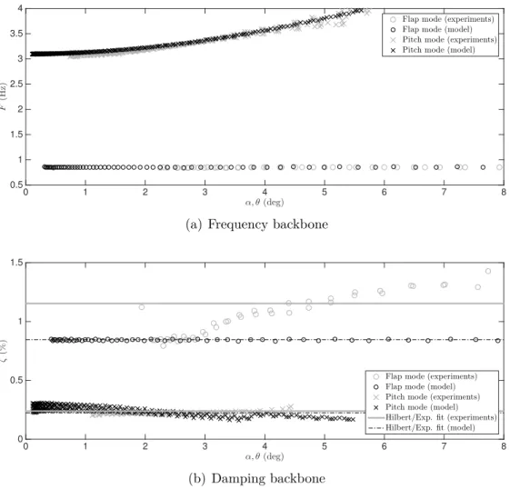
2.7.1 Wind-off frequency and damping backbones . . . 48
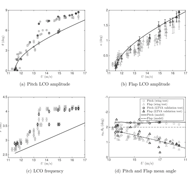
2.7.3 Post-critical response . . . 49
2.8 Chapter summary . . . 53
3 Flutter and LCO suppression on a pitch and flap wing 55 3.1 Introduction . . . 55
3.2 Mathematical model . . . 56
3.3 Linear absorber optimisation . . . 58
3.3.1 Effect of the absorber frequency and damping . . . 58
3.3.2 Effect of the absorber mass and length . . . 62
3.3.3 Effect of the absorber position . . . 64
3.4 Bifurcation analysis . . . 65
3.4.1 Post-critical response using linear absorbers . . . 65
3.4.2 Post-critical response using nonlinear absorbers . . . 68
3.5 Experimental absorber validation . . . 74
3.5.1 Linear absorber design and identification . . . 74
3.5.2 Effect of the absorber on the flutter speed of the system . . . 77
3.5.3 Effect of the absorber on the post-critical response of the system . . 78
3.6 Chapter summary . . . 81
4 Analysis and modelling of a pitch-plunge-control wing 83 4.1 Introduction . . . 83
4.2 Theoretical background . . . 84
4.2.1 Equations of motion of an aeroelastic system with freeplay and preload 84 4.2.2 Fixed points . . . 87
4.2.3 Two-domain and three-domain limit cycles . . . 89
4.3 Experimental setup . . . 90
4.4 Post-critical aeroelastic investigation . . . 92
4.5 Mathematical model of the experiment . . . 96
4.6 Bifurcation analysis using equivalent linearisation . . . 97
4.7 Numerical model validation . . . 102
4.7.1 Pre-critical response . . . 102
4.7.2 Post-critical response . . . 102
4.8 Chapter summary . . . 107
5 LCO suppression on a pitch-plunge-control wing 109 5.1 Introduction . . . 109
5.2 Mathematical model . . . 110
5.4 Linear tuned vibration absorbers investigation . . . 116
5.4.1 Critical airspeed optimisation . . . 116
5.4.2 Bifurcation analysis . . . 117
5.5 Nonlinear tuned vibration absorber investigation . . . 121
5.5.1 Cubic hardening NLTVA . . . 121
5.5.2 Freeplay NLTVA . . . 123
5.6 Chapter summary . . . 128
6 Conclusions 129 6.1 Suggestions for future work . . . 131
A Wind tunnel of the University of Li`ege 135
B Wind tunnel of the University of Duke 139
C Equations of motion of the pitch-flap wing 141
D Equations of motion of the pitch-plunge-control wing 145
E Publications 151
Chapter 1
Introduction
1.1 Aeroelastic problems throughout history
Most theses ever written about aeroelasticity start from Collar’s triangle [1]. This one makes no exception. Introduced in 1946 and depicted in figure 1.1, the triangle defines the aeroelasticity as the branch of physics that involves the combination of structural, inertial and aerodynamic forces.
Structural Mechanics Elastic forces Fluid Mechanics Aerodynamic forces Dynamics Inertial forces Aeroelasticity Forced response Flutter Static aeroelasticity Aer odynamic stabil ity Struc tur al v ib ration s
Figure 1.1: Collar’s triangle of forces [1]
Even though it was not named as such yet, static aeroelasticity was discovered centuries ago when aerodynamic structures such as wind mill blades and sails had to withstand wind loads. Static aeroelasticity was actually one of the major design parameters of the first aircraft whose very low thrust required very light structures and therefore very low
structural strength. The Langley machine (figure 1.2(a)), for instance, crashed on the Pomotac river in 1903 because of a classical torsional divergence of the wing [2, 3]. This phenomenon occurs when the torsional stiffness of the wing is lower than the aerodynamic moment, resulting in a diverging response that leads to the destruction of the wing. Sim-ilarly, the Foker D8 (figure 1.2(b)) suffered from flexural wing failure during high load manoeuvres because the lack of sufficient torsional stiffness of the wing combined with the aerodynamic loads led to an increase in the angle of attack of the wing tips, resulting in flexural loads larger than designed [4]. A similar phenomenon, due to the lack of sufficient torsional stiffness, is control surface reversal where the moment induced by the deflection of the control surfaces leads to a wing twist that reduces the wing tips’ angle of attack, which counters the effects of the control surface.
(a) Photograph of the Langley machine instants
before its crash. (b) Photograph of a Foker D8 aircraft.
Figure 1.2: Aircrafts featuring static aeroelastic problems. Credits: Wikipedia
As airplanes became more powerful, stiffer and faster, inertial forces started playing a role and aircraft designers were faced with a novel dynamic aeroelastic phenomenon: flut-ter. This phenomenon occurs when two or more natural frequencies of vibration of an aeroelastic system approach each other because of the wind loads and start exchanging energy between them and with the airflow, resulting in a exponential increase in vibration amplitude that usually leads to the loss of the aircraft. Figure 1.3 depicts a typical flut-ter case on an fundamental aeroelastic system with two modes of vibration. At wind-off conditions and below the flutter speed, the modes have well separated frequencies and positive damping ratios. As a result, the response of the system to non-zero initial con-ditions is a decaying oscillation (blue case). As the airspeed increases, the frequency gap between the modes decreases, the damping ratio of mode 1 increases and the damping ratio of mode 2 increases at first then decreases. When the airspeed reaches exactly the
1.1 Aeroelastic problems throughout history 3
system’s linear flutter speed, the modal damping of mode 2 is exactly equal to zero (or-ange) and a constant amplitude oscillation can be observed. For any airspeed higher than that, the system features a negative damping ratio in mode 2 and a response amplitude that exponentially diverges as time passes is observed (red). One of the first observations of such phenomena is the elevator-fuselage flutter that occurred on the Handle Page 0/400 during World War I [5]. The problem was solved by connecting the two elevators to the same torque tube, suppressing the anti-symmetric vibration mode of the elevator. Nowa-days, aircraft still undergo complex and expensive flight flutter test campaigns to certify that that no point of the flight envelope is closer than 80% (civil) or 85% (military) to the lowest flutter speed of the aircraft [6, 7]. Note that such phenomena are not limited to aircraft as long span bridges can also undergo, among other aeroelastic instabilities, flutter because of the combination of torsional and flexural modes [8–10].
Figure 1.3: Linear flutter of a two-DOFs aeroelastic system
The fact that an aircraft is futter-free does not mean that it cannot undergo other, less dangerous aeroelastic instabilities. Nonlinearities present in the structure or in the
air-flow can indeed cause Limit Cycle Oscillations (LCOs) at airspeeds lower than the linear flutter speed of the system. Such LCOs can lead to structural failure, aircraft re-design, flight envelope limitations or increased maintenance. Four decades after the first flights of the F-16, the aircraft still undergoes LCOs during certain manoeuvres at certain flight conditions with certain payloads that are most likely the result of aerodynamic missile -wing interactions, transonic effects and nonlinear friction in the bolted connections but which are still not fully understood. On the other hand, the F-18 (figure 1.4) aircraft suffers from vertical tail buffeting during certain high angle of attack manoeuvres because the fundamental frequency and location of vortices generated by the plane’s leading edge extensions coincides with that of the fins. Flutter is not limited to wings and control surfaces as skin panels flutter and LCOs can also be observed in numerous cases, most often in supersonic flight conditions. The clamping conditions of the panels usually in-troduce a hardening nonlinearity that limits the amplitude of the oscillations but can also lead to buckling when thermal effects are considered, which may significantly reduce the instability onset speed and cause chaotic oscillations because of snap-through phe-nomena. Depending on the amplitude and duration of the phenomena, panel LCO can result in structural failure. For instance, this phenomenon was judged dangerous for the X-15 aircraft and required a stiffening of the structure [11] but, on the other hand, it was judged non-destructive on Saturn V’s third stage because the amplitude and duration of the vibrations were not critical enough to cause structural failure [12]. In this case, hard-ening nonlinearities can have a beneficial effect because they limit the amplitude of the oscillations but panel buckling due to thermal stresses can also decrease the onset speed of the instability and require particular attention. A backlash or freeplay nonlinearity also caused the loss of a F-117 stealth aircraft during an airshow in 1997 [13]. The aircraft took off without any issue after the maintenance crew forgot to tighten four of the right aileron’s bolts, then a large amplitude LCO occurred during a particular manoeuvre and the wing broke into pieces, resulting in the loss of the aircraft.
1.2 State of the art in nonlinear aeroelasticity
As briefly introduced earlier, linear and nonlinear flutter can totally destroy aeronautic structures and should be avoided at all costs. As a result, it has received a lot of at-tention in the scientific community. This section presents an overview of the beneficial and detrimental effects that nonlinearities can have on the aeroelastic response of aircraft and introduces many nonlinear terms that are used in the thesis. The ultimate goal of this thesis is the study of dynamic absorbers, which are highly sensitive to the system’s natural frequencies and far less sensitive to the system’s damping ratios. As a result, the
1.2 State of the art in nonlinear aeroelasticity 5
Figure 1.4: Photograph of a F-18 aircraft at high angle of attack with smoke generators showing the leading edge vortex breakdown on the vertical tail. Credits: NASA Photo accent is put on stiffness nonlinearities rather than damping nonlinearities.
1.2.1 Linear flutter
If linear flutter remains a challenge in complex structures, the basic theory is now well un-derstood and the aeroelastic response of simple 2-DOF (degree of freedom) or 3-DOF sys-tems or of simple continuous wings is very well described in several good textbooks [14–18]. Figure 1.5 plots the bifurcation diagram (LCO amplitude variation with airspeed) of a typical linear aeroelastic system. At airspeeds lower than UF, the linear flutter speed of the system, the modal damping of all the modes is positive and the response to a pertur-bation is a decay to a stable fixed point, which is a static equilibrium of the equations
of motion that can attract a response trajectory. At the airspeed UF, a degenerate Hopf
bifurcation occurs, the fixed point becomes unstable, the modal damping of one of the modes is exactly equal to zero and circles whose amplitudes depend on the initial condi-tions are observed. At any airspeed larger than the flutter speed, a diverging response is observed. Note that linear flutter only exists mathematically as nonlinear phenomena such as stall, hardening/softening nonlinearities or structural failure will always affect the amplitude of the oscillations in real life applications.
1.2.2 Nonlinear aeroelasticity
The presence of nonlinearities in the structure or in the airflow significantly affects the aeroelastic response of the system. Depending on the nature of the nonlinearities, they can
0
Airspeed
A
mplitude
U
Fixed point (stable) Fixed point (unstable) LCO (stable) LCO (unstable)
F Diverging oscillations
Figure 1.5: Typical bifurcation diagram of a linear aeroelastic system
lead to LCOs at airspeeds lower than the system’s linear flutter speed but also usually limit the amplitude of the response compared to linear flutter. In this section, a non exhaustive review of the relevant nonlinearities is discussed along with the dedicated studies.
Smooth nonlinearities
Continuous nonlinearities were first considered for their simplicity and because they rep-resent geometric nonlinear phenomena associated with large displacements. Figure 1.6 depicts typical hardening and softening smooth nonlinearities. The restoring force is hardening when an increase in amplitude leads to an increase in the slope of the restoring force and therefore to an increase in instantaneous frequency or softening when it is the opposite. Many authors investigated such nonlinearities on systems with pitch and plunge DOFs, starting with Woolston et al. in 1955 [19] using an experimental apparatus and analog computers and McIntosh et al. in 1981 [20], who designed an apparatus than can feature many different types of linearities by changing simple elements, including con-tinuous hardening. These first studies focused on the onset speed of the LCOs rather than on their amplitude variation with airspeed. Then, the Texas A&M department de-signed the Nonlinear Aeroelastic Testbed Apparatus (NATA), a system that uses cams and wires to generate any desired continuous nonlinearity [21–23] and Abdelkefi et al. [24] obtained very good experiment/mathematical model agreement on a system with cubic and quadratic stiffness. Price et al. [25] also demonstrated that hardening systems can undergo smooth LCOs in a wide airspeed range but also aperiodic or chaotic oscillations at airspeeds above the system’s torsional divergence speed because of a pitchfork bifurca-tion.
1.2 State of the art in nonlinear aeroelasticity 7 Angle For ce Linear Hardening Softening
Figure 1.6: Typical smooth nonlinear restoring forces
0
Airspeed
A
mplitude
U
Fixed point (stable) Fixed point (unstable) LCO (stable) LCO (unstable)
F
(a) Super-critical Hopf bifurcation
0 Airspeed A mplitude UF UA
(b) Sub-critical Hopf bifurcation
Figure 1.7: Typical bifurcations diagrams observed with continuously nonlinear aeroelastic systems
LCOs” and ”bad LCOs” [22]. Good LCOs (see figure 1.7(a)) arise at UF, the linear
flut-ter speed of the system (i.e. the flutflut-ter speed of the underlying linear system), because of a supercritical Hopf bifurcation and propagate in the increasing airspeed direction. As a result, at airspeeds below the Hopf speed, the response of the system to non-zero initial conditions will always decay to a fixed point and at airspeeds above the flutter speed, the response of the system to non zero initial conditions will stabilise to a LCO. In this case, the nonlinearity has a beneficial effect on the system since it does not induce any LCO at airspeeds below the flutter speed but limits the amplitude at higher airspeeds.
Bad LCOs (see figure 1.7(b)) arise at UF because of a sub-critical Hopf bifurcation
and propagate in the decreasing airspeed direction then usually change direction because
bi-furcation is usually unstable and becomes stable after the fold. As a result, below the airspeed UA, the response of the system decays to the fixed point irrespective of the initial
conditions. At airspeeds between UA and UF, the system can undergo LCOs or decay to
the fixed point depending on the initial conditions and at airspeeds above UF only LCOs
can be observed. The airspeed region between UA and UF is referred to as a bi-stable
region because LCOs can be observed depending on the initial conditions. Due to the sub-critical nature of the Hopf bifurcation, LCOs can be observed at airspeeds smaller
than the system’s Hopf point. As a result, the limiting airspeed is UA, the LCO onset
speed, which is the smallest airspeed at which LCOs can be observed.
The origin of such supercritical and subcritical phenomena can be explained by looking at the system’s natural frequencies variation with airspeed. Figure 1.3 plots an aeroe-lastic systems’ modal frequency variation with airspeed. Linear flutter is observed at an
airspeed UF because of the combination of mode 1 and mode 2. If mode 1 is hardening
and/or if mode 2 is softening, an increase in amplitude would tend to separate the natural frequencies of the system irrespective of the airspeed and no LCO can be observed below the linear flutter speed. As a result, the system would behave as in figure 1.7(a), i.e. only
fixed point solutions exist between airspeeds 0 and UF. Above the linear flutter speed
of the system, the nonlinearities tend to stabilise the system and LCOs are observed. Conversely, if mode 1 is softening and/or mode 2 is hardening, an increase in amplitude at airspeeds lower than the flutter speed would reduce the frequency gap between the modes and may cause LCOs at airspeeds smaller than the flutter speed. As a result, bifurcation diagrams similar to that displayed in figure 1.7(b) can be observed. Between airspeeds of 0 and UA, the frequency gap is large enough to avoid flutter irrespective of
the amplitude. Between airspeeds of UA and UF, the natural frequencies of modes 1 and
2 are close but not enough to flutter. If the amplitude is increased, the frequency gap is
decreased and LCOs can occur. For airspeeds above UF, linear flutter has occurred and
only LCOs can be observed. In real life applications, there usually are more than two modes and a hardening nonlinearity on mode 1 might lead to sub-critical LCOs because of the coalescence of this mode with another mode of higher frequency and the same phenomenon may happen with mode 2 and a softening nonlinearity.
Non-smooth nonlinearities
Freeplay nonlinearities feature a bi-linear stiffness which is zero within the freeplay gap of width 2” and non-zero outside (see figure 1.8). If the freeplay spring is placed in parallel with a linear spring, the full restoring force is bilinear and while a ”freeplay” or ”flat spot” restoring force is considered when the structural stiffness is equal to zero inside the
1.2 State of the art in nonlinear aeroelasticity 9
freeplay gap. Such bilinear restoring forces can be studied by de-coupling the system into two linear sub-systems. The underlying linear system is the system whose response lies within the freeplay boundaries while the overlying linear system is the system with full stiffness, when the freeplay gap width is equal to zero, i.e. when the aircraft performs in a normal way. Angle For ce Overlying linear Underlying linear Nonlinear 2δ
Figure 1.8: Typical freeplay nonlinear restoring forces
0 Airspeed A mplitude UF1 UF2 δ UA LCO (stable) LCO (unstable)
Figure 1.9: Typical bifurcations observed in systems with freeplay in pitch
Figure 1.9 depicts a sub-critical bifurcation characteristic of symmetric wing section with pitch and plunge degrees of freedom and with freeplay in pitch. At UF,1, the flutter speed of the underlying linear system, three unstable LCO branches emanate from a grazing bifurcation. Two of these branches are highly asymmetric and investigated in detail in chapter 5 and in [26] on a similar system while the amplitude variation with airspeed of the symmetric branch is depicted in figure 1.9. The small amplitude highly asymmetric limit cycles are referred to as two-domain LCOs and orbit around points lying just out-side the two boundaries while the large amplitude LCO is referred to as a three-domain
LCO and orbits around zero. After the bifurcation, an unstable LCO branch propagates
in the decreasing airspeed direction until airspeed UA where a fold bifurcation occurs,
which changes the branch stability and propagation direction. Then, the LCO amplitude increases smoothly with airspeed and asymptotically becomes infinite at UF,2, the flutter speed of the overlying linear system. Note that for such phenomena to occur, the un-derlying linear system’s flutter speed must be smaller than that of the overlying linear system. One of the major differences between systems with freeplay and systems with smooth nonlinearities is that, since LCOs can only be observed on nonlinear systems, the first limit cycle that emanates from the bifurcation cannot have an amplitude equal to zero as it must enter and exit the freeplay region.
Such nonlinearities usually lead to LCOs at airspeeds lower than the linear flutter speed of the overlying linear system, which makes them potentially dangerous. As a result, the FAA authorities place very strict limits on the amount of freeplay allowed in aircraft control surfaces (see [27]) and a lot of research has been devoted to this subject, usually on simple systems featuring 2 or 3 DOFs.
Some of the first studies where conducted by Woolston et al. [19] and by McIntosh et al. [20] on pitch and plunge wings with freeplay in pitch. The authors focused on the onset speed of the instability. Yang et al. [28] studied the whole branch using the Har-monic Balance method. Hauenstein et al. [29], Price et al. [25], Liu et al. [30] and Chung et al. [31] then demonstrated numerically and experimentally the existence of aperiodic oscillations, most likely because of the coexistence of several stable fixed points. Experi-ments performed by Marsden et al. [32] with various freeplay gaps demonstrated that the LCO amplitude depends linearly on the width of the freeplay gap and that the smaller the gap, the higher the LCO onset speed. The authors concluded that this increase in LCO onset speed with small freeplay gaps was due to nonlinear bearing damping.
Systems with a higher complexity but still freeplay in pitch were then considered. Chen et al. [33] observed the co-existence of chaos and LCOs on a pitch-plunge wing with freeplay in pitch and with an external store. Tang et al. [34] combined the ONERA stall model [35] on a helicopter blade with freeplay in pitch and with a flap DOF. They observed that chaos was dominant at small amplitude with the freeplay model and at high amplitude with the stall model. Flexible control surfaces with freeplay in pitch were used by Kim et al [36] and Tang et al. [37,38]. The authors observed that the flexibility of the surface has a significant effect on the linear flutter behaviour of the system but does not affect much the system’s response when freeplay is also considered. The latter authors also observed
1.2 State of the art in nonlinear aeroelasticity 11
that the LCO onset speed increases with the aerodynamic preload, which led Chen et al. [39] to state that the military freeplay specifications are too strict after a similar study on a F-16 model with freeplay in the control surfaces.
The effect of freeplay in the control surface was investigated by many researchers using the typical aeroelastic surface [40], a rigid 2D wing featuring pitch, plunge and control surface deflection DOFs with freeplay in the control surface. Theoretical models and experiments were used to understand the aeroelastic response of the system, which features complex branches that appear and disappear [40–42] but also to validate numerical methods used to tackle aeroelastic problems and the discontinuities inherent to freeplay [43–47]. One of the major differences between this system and those with freeplay in pitch is that the underlying linear system features not one but three stability changes, two of which are due to plunge-control surface flutter and the third is due to pitch-control surface flutter. As a result, the system features two branches of limit cycles that are able to interact with each other, resulting in complex behaviour.
Subsonic aerodynamic nonlinearities
The main source of subsonic aerodynamic nonlinearities is separation of the airflow. Such separation usually occurs around bluff bodies or around streamlined bodies at high angles of attack. Depending on the geometry of the objects, this separation of the airflow can lead to several types of aeroelastic instabilities. Galloping and vortex induced vibration (VIV) are translational instabilities that occur in a direction perpendicular to that of the mean airstream. Separated airflows usually have a natural frequency, which is re-lated to the Strouhal number. In the case of galloping, the fluid’s natural frequency is usually higher than that of the structure and the instability, whose amplitude increases with airspeed once the critical airspeed has been reached, is due to a negative damping provided by the airflow. Vortex induced vibration (VIV) on the other hand, occurs when the shedding frequency of the Von Karman vortices is close to one of the translational natural frequencies of the structure. In that case, a coupling between the fluid and the structure can occur, resulting in a lock-in phenomenon and large amplitude LCOs in a given airspeed range. Slender civil engineering structures such as bridges, cables and tall towers are typically prone to such instabilities however, they are usually not encountered in aerospace structures because they are streamlined. Stall flutter, on the other hand, is a rotational instability due to dynamic stall, which can occur on buff bodies but also on streamlined bodies such as wings or helicopter blades at high angle of attack. As a result, it has received much more attention in the aerospace community. Owing to the high complexity of the involved phenomena, a lot of research has been conducted on dynamic
stall, which is an unsteady aerodynamic phenomena occurring under forced motion, but not so much on stall flutter, which is an aeroelastic phenomenon involving the coupling of dynamic stall with the dynamics of a flexible structure. Note that unlike all the non-linearities investigated above, flow separation can cause instabilities on systems featuring a single structural mode.
AOA C Static Dynamic 1.5 1 0.5 N 5 0 10 15 20 25 A B C D E F G
(a) Normal force coefficient
AOA C -0.1 -0.2 -0.3 M 5 0 10 15 20 25 B C D E F G A E’
(b) Pitching moment coefficient
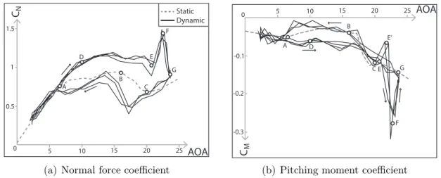
Figure 1.10: Static and dynamic normal force and pitching moment of a S809 profile undergoing a dynamic stall test
Figure 1.10 depicts the variation of the normal force coefficient (force perpendicular to the wing), CN, and pitching moment coefficient around the quarter chord, CM, with angle off attack (AOA) of a S809 wind turbine blade, obtained from the National Renewable En-ergy Laboratory (NREL) [48]. The grey curves correspond to static tests while the black lines correspond to dynamic tests performed by continuously varying the AOA between
2¶ and 24¶ at a reduced frequency k = Êb/U = 0.0335, where Ê is the forcing frequency,
b is the half-chord and U is the airspeed. Unlike the static measurements, the dynamic
data feature hysteresis and the path indicated by the arrows corresponds to an AOA that is equal to 2¶, increases to 24¶ and eventually decreases back to 2¶.
The static normal force increases linearly with the pitch angle up to AOA = 6¶ (A), the
static stall angle, then slowly varies up to AOA = 16¶(B), drops until AOA = 20¶ (C) and
increases smoothly with the AOA at higher angles. The smooth load variation with AOA above the stall angle is due to the thickness and to the ”whale” shape of the airfoil profile, which induces a separation from the trailing edge that slowly reaches the leading edge as the AOA is increased. Thinner profiles such as the widely studied NACA 0012 lead to a more abrupt stall (see the work of McAlister, Mcroskey et al. for instance [49–51]).
1.2 State of the art in nonlinear aeroelasticity 13
The moment coefficient is relatively low at small angles because the moment is measured
around the wing’s quarter chord. At AOA = 6¶ (A), stall occurs and the moment starts
to increase with the AOA. Right after point (B), the moment starts to drop because the aerodynamic center moves towards the trailing edge of the wing.
The dynamic test results are quite different from the static ones and three key phe-nomena inherent to dynamic stall are observed: stall delay, leading edge vortex (LEV) and re-attachment. In the dynamic case, the lift increases linearly with the AOA up to
AOA = 10¶ (D) before stall begins to saturate the lift force. This phenomenon, known
as stall delay, can be due to viscid (see McCroskey [52]) and inviscid boundary layer (see Ericsson and Reding [53]) contributions and can lead to maximum aerodynamic loads much higher (approximately 25% in this case) than predicted using steady data. Between
AOA = 10¶ and AOA = 21¶, the separation point moves towards the wing’s leading edge
and a leading edge vortex (LEV) starts forming. At AOA = 21¶ (E), the separation point
reaches the leading edge of the wing and the LEV detaches from the wing, is convected downstream and creates a strong suction effect that greatly increases the aerodynamic
load. At AOA = 23.4¶ (F), the LEV is at the trailing edge of the profile and leaves
the wing, which leads to a rapid decrease of its effect. At 24¶, the LEV is already far
enough from the wing to have a negligible effect. The width of the LEV-induced peak is directly dependent on the reduced frequency and its strength induces maximum normal forces 58% higher than the static predictions. When the AOA decreases, re-attachment starts to occur at an angle that is different from the stall angle and that lies between 6¶,
the static stall angle, and 10¶. Unlike the stall angle which is approximately the same at
each cycle, the re-attachment angle is different from one cycle to the next but remains within a bounded space.
Those three dynamic stall phenomena are also observed on the moment curves. Even though those data are nosier than the normal force ones, point D appears to be aligned with the static curve owing to the stall delay phenomenon. The LEV is shed at point E, increases the moment at first because it is located in front of the quarter chord (point
EÕ) then leads to a large drop in moment as its strength and distance from the quarter
chord increases. The dynamic moment is around twice as high as the static predictions. When the angle decreases, the moment increases to values similar to the static ones and the re-attachment process begins.
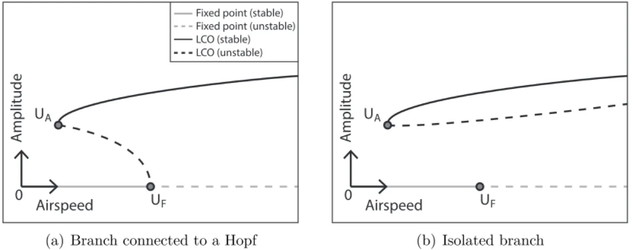
Combining dynamic stall with a linear flexible structure with, for instance, pitch and plunge DOFs can cause stall flutter which leads to bifurcation diagrams similar to those
0 Airspeed A mplitude UF UA
Fixed point (stable) Fixed point (unstable) LCO (stable) LCO (unstable)
(a) Branch connected to a Hopf
0 Airspeed A mplitude UF UA (b) Isolated branch
Figure 1.11: Typical bifurcations observed in nonlinear systems undergoing stall flutter
depicted in figure 1.11. At airspeeds smaller than UA, the aerodynamic loads are not
sufficient to cause stall flutter irrespective of the initial conditions imposed on the wing.
At airspeeds between UA and UF (the linear flutter speed of the system), large enough
initial perturbations can cause LCOs while small initial perturbations lead to decaying responses. At airspeeds above UF, linear flutter has occurred, the fixed point is unstable and the amplitude of the oscillations increases until it stabilises on a limit cycle. In this case, the stall phenomena have a beneficial effect because they limit the amplitude of the oscillations, which would diverge if linear aerodynamics were considered. In figure 1.11(a), the LCO branch is connected to the Hopf point associated with the system’s linear flutter speed and a sub-critical Hopf bifurcation is observed while in figure 1.11(b), the LCO branch is not connected to the Hopf point and is referred to as an isolated solution branch or isola. Stall flutter can of course also occur on systems with other additional nonlinearities, resulting in complex bifurcation behaviours combining the branches of fig-ure 1.11 with smooth or non-smooth nonlinearities (figfig-ures 1.7 and 1.9) that lie underneath the stall flutter branches.
Because of the complexity of stall flutter phenomena, full aeroelastic studies are usually limited to simple wings with few DOFs. The ONERA dynamic stall model, introduced by Tran et al. [35] has been coupled to flexible structures by several authors. Tang et al. [34, 54] performed experiments and computations on a helicopter blade, achieved a good experiments - model correlation and observed that chaos could arise at sufficiently high LCO amplitudes. Dunn et at [55] studied numerically and experimentally the re-sponse of a cantilever wing with a NACA0012 profile and focused on the effect of the mean angle of attack of the wing on the reponse. Dimitriadis and Li [56] performed experiments
1.3 Vibration mitigation techniques 15
on a NACA 0012 airfoil and observed that fixed points, symmetric LCOs, and strongly asymmetric LCOs could co-exist depending on the airspeed. The authors also observed that all limit cycles demonstrate a certain amount of cycle-to-cycle variability, probably because of the non-repetitive nature of the re-attachment phenomenon. They also ob-served the travel of the leading edge vortex by means of pressure transducers. Similar experiments performed by Abdul Razak et al. [57] on a NACA 0018 airfoil with pitch and plunge DOFs highlighted that the higher (in absolute value) the mean pitch angle, the lower the stall flutter airspeed but also the smoother the LCO amplitude variation with airspeed. They also observed that the LCO frequency of wings undergoing stall flutter is closely related to that of the linear flutter speed of the same system, which suggests that the two phenomena are linked.
1.3 Vibration mitigation techniques
1.3.1 Active control
The basic principle of active flutter control consists in measuring the aircraft’s response in real time and applying a feedback force in order to increase the flutter speed or de-crease the LCO amplitude. Figure 1.12 depicts a typical control loop where a controller records the system’s accelerations and velocities and applies an input force on the system, usually thanks to minijets, piezoelectric actuators or control surfaces. Thorough intro-ductions into the subject are available in Dowell et al. [17] and Wright and Cooper [18]. Most modern aircraft feature Flight Control Systems (FCS) that integrate some sort of feedback using accelerometers or gyroscopes and control surface deflections in order to enhance the flying qualities or the gust response of the aircraft however these systems are not designed to affect the structural modes and the flutter properties of the aircraft, probably because it is not permitted by the airworthiness regulation authorities and be-cause a failure in the system would result in the loss of the aircraft. Nevertheless, active flutter control has been widely studied by the scientific community using numerical mod-els, wind tunnel experiments and even flight tests. The goals of these studies were mainly to demonstrate the potential of the technique, to compare the performance of different control lows and to test various methods of applying control forces.
The most straightforward way of applying control forces is using the aircraft’s existing control surfaces, which means that it might be feasible to implement such active control systems without significant modifications of the structure. Borglund et al. [58] and Yu et al. [59] achieved an increase in flutter speed of 50% and 13.4%, respectively, numerically
Aeroelastic system External forces
Control system
System response (y y) Control forces
Figure 1.12: Block diagram of an aeroelastic system with a control loop
and in the wind tunnel. The former authors nevertheless suspect that the very good per-formance of their control system is due to a weak flutter mechanism. Mukhopadhyay [60] used the PAPA (Pitch And Plunge Apparatus) in a transonic wind tunnel and achieved an increase in critical airspeed of at least 20% (wind tunnel limitations did not allow to test at sufficiently high airspeeds). Huang et al. [61] studied the effect of time delay in the control loop. The authors showed numerically that an increase in flutter speed of 19% with a sufficiently fast controller can be achieved but also that a controller whose response is too slow can decrease the system’s flutter speed. Sensburg et al. [62] performed flight tests on a F4 Phantom fighter jet and were able to increase the aircraft’s flutter speed by 16%. Nevertheless, three backup flutter suppression mechanisms were implemented to guarantee the safety of the test.
Piezoelectric actuators can also be used to apply the necessary control forces. In this case, the aeroelastic control loop does not interact with the FCS. Han et al. [63] achieved an increase in flutter speed of between 6 and 11% depending on the control law and Moses [64] performed wind tunnel tests on a 1/6 scale model of a F-18 undergoing tail buffeting. Piezoelectric actuators and control surface actuators both led to a decrease in root RMS (root mean square) amplitude of about 60%.
1.3.2 Passive control via structural aircraft modifications
To this day, no active control solution has been approved for use on aircraft by airwor-thiness regulation authorities and the only possibility to increase the flutter speed of an aircraft is a structural re-design of the components that interact to cause the instability. Generally, flutter can be avoided by increasing the stiffness of the structure (at the cost of increased weight) or by reducing the coupling between the relevant structural modes. This can be done either by adding masses at certain strategic locations or by displacing the elastic axis of the structure. The former method, called mass balancing, is often used for
1.3 Vibration mitigation techniques 17
control surfaces. An example of control surface masses is depicted in figure 1.13. With the increasing amount of composite materials used in aerospace structures, aeroelastic tailoring, which consists in optimizing the composite structure while taking aeroelastic contraints into account, is another potential technique for flutter speed optimisation [65].
Figure 1.13: Photograph of the balancing masses on the control surfaces of a Messerschmitt 110 aircraft. Credits: Wikipedia
Usually, increasing the modal damping of the system may also increase the flutter speed and/or reduce the LCO amplitude. Cunha et al., for instance, tested numerically the effect of viscoelastic materials in a sandwich configuration to mitigate panel flutter [66]. Malher et al., on the other hand, used a shape memory alloy on a 2-DOF aeroelastic apparatus in order to introduce hysteretic dissipation, resulting in increased flutter speed and decreased LCO amplitude [67,68].
1.3.3 Passive control via dynamic absorbers
Yet another option to mitigate LCOs, which is investigated in detail in this thesis, is the use of dynamic absorbers. Figure 1.14(a) depicts a generic 1-DOF system, called the primary system, with a dynamic absorber made of a mass attached to the primary system by means of linear or nonlinear stiffness and damping couplings. Depending on the couplings chosen, very different properties can be obtained. Such absorbers have received a lot of attention in the civil and mechanical engineering communities however very few studies are available for aircraft flutter suppression. Table 1.1 summarises all the absorbers considered in this literature review and their stiffness and damping properties.
Classical mass dampers
Absorber Stiffness force Damping force
LTVA (Frahm) [69] Linear
-LTVA [70–74] Linear Linear
Cubic NES [75–83] Purely cubic Linear
Damping NES [84] Linear Quadratic
Impact NES (VA) [85] Impact Impact
Hysteretic TMD [86] Hysteresis Hysteresis
NLTVA [87–92] Linear + Polynomial Linear
Special mass dampers
Membrane NES [93] Grounded cubic Linear
LTVA + Impact [94] Linear + Impact Linear + Impact
Table 1.1: Summary of the dynamic absorbers used in the literature Linear absorber
A Linear Tuned Absorber (LTVA) also called Tuned Mass Damper (TMD) is obtained when the absorber mass is connected to the primary system using a linear spring and dashpot. Introduced by Frahm in 1911 [69] and upgraded by Ormondroyd in 1928 [70], this absorber is capable of splitting a large amplitude resonance peak of the primary sys-tem’s frequency response function (FRF) into two small amplitude peaks, provided its natural frequency and damping ratio are tuned in accordance to those of the primary system. The equal peaks method, approximated by Den Hartoog and Brock [71, 72] and derived in an exact form by Asami [73], allows to rapidly tune the absorber’s stiffness and damping. This absorber provides a large amplitude reduction however a very accurate tuning of the stiffness is required and the LTVA is only effective on one mode while the structure might feature several potentially dangerous modes. Moreover, in the presence of structural nonlinearities, the change in natural frequency of the primary system with amplitude of oscillation can be sufficient to detune the absorber, thus greatly reducing the resulting dissipation. TMDs are widely used in high towers and bridges for vortex-induced-vibration (VIV) or human-induced vibration [95–100]. Bridge torsion-flexure flutter has also been considered by Gu et al. [9]. The authors showed mathematically and in the wind tunnel that an increase in flutter speed of 40% was achievable with TMDs weighing 5.6% of the total mass of the bridge. Kwon et al. [101], performed a similar study however many TMDs with smaller masses were considered rather than one or two absorbers. The authors showed that by optimising the natural frequencies and damping
1.3 Vibration mitigation techniques 19
ratios of the smaller absorbers, it is possible to increase the robustness of the system. Another example demonstrating the performance of the TMD can be found in formula one. Such absorbers were fitted on the Renault R26 car at the end of the 2005 season to mitigate the vibrations induced by the kerbs, thus increasing the mechanical grip and downforce consistency on the car’s front and back ends. They were then banned in the middle of the 2006 season, after other teams failed to achieve Renault’s performance and complained to the international automobile federation.
Even though they are effective in a narrow frequency band, such absorbers can increase the flutter speed of 2-DOF systems by a large amount. The first aeroelastic study, con-ducted by Karpel [102] in 1981, demonstrated that an increase in flutter speed of 62% could be achieved using an absorber weighing 20% of the total mass of the system however, as in mechanical engineering, a small change in the absorber’s or in the primary system’s natural frequency led to a large decrease in performance. The absorber was tuned by computing the variation of the flutter speed of the coupled system with absorber natural frequency and damping ratio, i.e. by trial and error. A LTVA made of a RLC (resistance, inductance, capacitance) resonant shunt circuit with piezoelectric materials was also con-sidered by Moon et al. to mitigate panel flutter [103]. The authors computed a reduction in LCO amplitude of 30% to 60% but were not able to increase the onset speed of the instability. Primary System Abs. y x f(x-y) f(x-y)
(a) Schematics of the system
F (Hz) 0.6 1 1.4 A/F ex t (m /N) 0 0.01 0.02 0.03 LTVA No Absorber (b) FRF of the system
Classical nonlinear energy sink
As the natural frequency of aeroelastic systems usually varies with flight condition and oscillation amplitude and since flutter is the result of the combination of two or more modes, it might be tempting to use an absorber featuring a linear damping force (for simplicity) and a purely cubic stiffness force. This absorber, which is referred to as a classical Nonlinear Energy Sink (classical NES), has been introduced by Roberson and studied by many authors in the mechanical engineering community ever since [75–80,83]. The absorber is capable of pumping energy out of a mode using Targeted Energy Transfer (TET) but, more importantly, it offers a broadband dissipation while the LTVA is only able to dissipate energy in a narrow frequency band. As a result, the NES is also widely studied in civil engineering for earthquake protection [104, 105]. The drawback of such absorbers is that their performance is amplitude-dependent and a threshold is usually required to achieve good performance.
Aeroelastic studies have been performed using such an absorber by Lee et al. [80–82] on the NATA system both numerically and experimentally. The authors showed an in-crease in flutter speed of about 3% numerically and 26% experimentally as well as a great reduction in LCO amplitude with NES weighting between 10% and 12.5% of the mass of the primary system. Hubbard et al. [83] demonstrated numerically and experimentally an increase in LCO onset speed of about 6% on a swept wing in the transonic regime using an absorber with a mass of only 1% of the total mass of the wing.
As mentioned earlier, the stability of a nonlinear system at very low oscillation amplitudes is identical to that of an underlying linear system, i.e. the Hopf bifurcation flight condi-tion of the nonlinear system is coincident with the flutter speed of the underlying linear system. As a result, it is possible to demonstrate that the NES can never outperform the LTVA in increasing the Hopf point airspeed using equivalent linearisation [106]. As-suming an aeroelastic system similar to that sketched in figure 1.14(a) undergoing a LCO described by the DOF y at a frequency Ê and a NES undergoing a displacement x, the relative displacement between the absorber and the primary system can be approximated using a sinusoidal assumption
x≠ y = A sin(Êt) (1.1)
where A is the amplitude of oscillation and Ê its frequency. The resulting NES restoring force, FNES, is given by
1.3 Vibration mitigation techniques 21
where k3 is the cubic restoring force coefficient which has been optimally tuned.
Substi-tuting equation 1.1 into equation 1.2, using trigonometric identities and neglecting the third harmonic (equivalent linearisation) yields
FN ES = k3A3sin3(Êt) = 1 4k3A3[3 sin(Êt) ≠ sin(3Êt)] ¥ 34k3A3sin(Êt) ¥ 34k3A2(x ≠ y) (1.3)
which means that for any LCO inducing a relative NES-primary system displacement of amplitude A, the NES’s restoring force can be approximated by a linear restoring force of equivalent linear stiffness keq = 34k3A2. As a result, at the flutter point, since it is reasonable to assume that A is very small, the NES behaves like a LTVA without stiffness, i.e. it can only be tuned in damping. In contrast, an LTVA can also be tuned in stiffness and therefore it will always outperform a NES in increasing the flutter speed.
Other nonlinear dynamic absorbers
Other types of nonlinear absorbers were also considered in the literature. Poovarodom et al. [84] used an absorber with linear stiffness and purely quadratic damping, corresponding to the drag of a plate immersed in a liquid, because it is easier to build than a LTVA. They showed that a performance similar to that of a LTVA can be obtained in a civil engineering case. Lacarbonara et al. [86] considered hysteretic forces and showed that they were able to provide additional dissipation compared to a LTVA. Ema et al. [85] considered an impact damper where most of the dissipation came from the contact between a mass and mechanical stops. This absorber was able to increase the damping in the system by a factor of 10 but again is probably not effective in delaying linear flutter because a minimum amplitude is required to trigger the NES. Collette et al. [94] countered the problem by attaching the impact damper to a linear absorber. As a result, the system behaves like a LTVA at small amplitude and like a coupled LTVA - impact damper at larger amplitude. Bellet et al. [93] also considered a NES made of a membrane coupled linearly to the primary system but with a grounded nonlinear restoring force in order to damp low frequency sound waves. Such complex NESs have not been investigated in the aeroelastic literature yet.
Nonlinear tuned vibration absorber
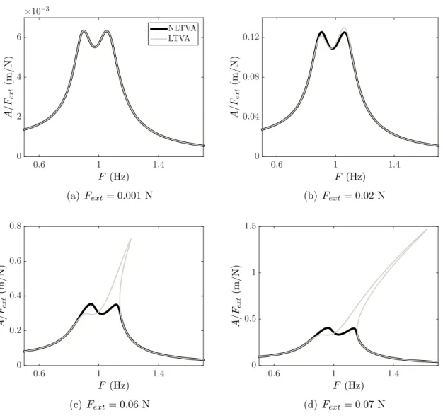
As stated earlier, the LTVA is very effective in a narrow frequency band while the classical NES is not effective in delaying the Hopf point but dissipates energy in a wide frequency band. Combining a classical NES with a LTVA results in a nonlinear tuned vibration ab-sorber (NLTVA) which offers better robustness than the LTVA and better low amplitude performance than the classical NES. The NLTVA was probably introduced by Robertson et al. in 1952 [87] who used it on a linear primary system to extend the frequency band where the absorber is effective. Many other studies followed on Duffing primary systems which consist of a linear 1-DOF oscillator with a cubic stiffness in parallel to the linear stiffness [88–92,107]. These studies showed that in the presence of a hardening or soften-ing nonlinearity, the LTVA can be effective at low forcsoften-ing amplitude but detuned when the forcing amplitude is increased. The addition of a NLTVA whose nonlinearity mimics the nonlinearity of the primary system can counter the effects of the nonlinearity in the primary system and greatly improve the absorber performance [92]. Figure 1.15 plots the FRF of a 1-DOF Duffing oscillator with LTVA (grey) and NLTVA (black) at 4 different forcing amplitudes. At low level (figure 1.15(a)), the linear and nonlinear absorbers per-form identically because the nonlinearity in the primary system is not effective. Then, the higher the forcing amplitude, the higher the detuning and the larger the difference in performance between the LTVA and the NLTVA (figures 1.15(b) to 1.15(d)).
The NLTVA was first tested in aeroelasticity by Habib et al. [108]. The authors used a Van der Poll-Duffing 1-DOF oscillator to mimic an aeroelastic system featuring a super-critical bifurcation and LCOs. They demonstrated that a LTVA was effective in increasing the LCO onset speed but turned the super-critical bifurcation into sub-critical. By adding a nonlinear restoring force, they could restore the super-criticality and decrease the LCO amplitude. Similar results were obtained by Malher et al. [109] on more realistic systems featuring pitch and plunge DOFs and hardening nonlinearities in pitch.
1.3 Vibration mitigation techniques 23 F (Hz) 0.6 1 1.4 A/ Fex t (m /N ) ×10−3 0 2 4 6 NLTVALTVA (a) Fext= 0.001 N F (Hz) 0.6 1 1.4 A/ Fex t (m /N ) 0 0.04 0.08 0.12 (b) Fext= 0.02 N F (Hz) 0.6 1 1.4 A/ Fex t (m /N ) 0 0.2 0.4 0.6 0.8 (c) Fext= 0.06 N F (Hz) 0.6 1 1.4 A/ Fex t (m /N ) 0 0.5 1 1.5 (d) Fext= 0.07 N
1.4 Objectives of the thesis
Nonlinear aeroelastic phenomena occur in real life applications and usually have to be avoided for safety, performance and maintenance reasons. Such phenomena are usually linked to linear flutter, smooth nonlinearities, freeplay, transonic effects, stall or buckling. Dynamic absorbers have proven to be effective tools in order to dissipate energy in me-chanical systems and civil engineering structures, however appart from a few pioneering studies, very little work has been carried out on the application of such absorbers on aircraft-like aeroelastic systems.
The goal of this thesis is to understand and demonstrate the performance of linear and nonlinear tuned mass dampers for flutter and LCO suppression. Two simple aeroelastic systems featuring different structural nonlinearities are investigated theoretically and ex-perimentally.
The first system is made of a flat plate with pitch and flap DOFs and a structurally hardening nonlinearity in pitch. This system features one of the simplest aeroelastic re-sponses possible and is therefore a good candidate for a first flutter suppression attempt. The system is first tested in the wind tunnel then modelled using simple aerodynamics. Subsequently, the mathematical model is used to investigate the performance of linear and nonlinear absorbers and to determine optimal tuning rules for the absorbers. Finally, the experimental apparatus is used again to demonstrate the performance of the absorber in the wind tunnel.
The second aeroelastic system is made of a rigid wing with pitch, plunge and control surface deflection DOFs with freeplay in the pitch DOF. This system features a much more challenging aeroelastic response featuring the co-existence of small and large am-plitude LCOs in a given airspeed range, aperiodic LCOs and up to three fixed points, depending on the aerodynamic preload. A similar approach is followed: the system is tested in the wind tunnel, then a mathematical model is derived and used to investigate the performance of the absorbers. No experimental validation was performed for this system.
Chapter 2
Design, analysis and modelling of a
pitch and flap wing
2.1 Introduction
In this chapter, a novel experimental aeroelastic setup with degrees of freedom in pitch and flap is proposed. Inspired by the wing designed by G.J Hancock in the eighties for teaching purposes [110], the system is made of a flat plate suspended from the roof of the wind tunnel of the University of Li`ege by means of a leafspring that provides a linear restoring force in flap and a continuously hardening restoring force in pitch. The advan-tage of this design is that it is simple, cheap and that is does not use any bearings. One of the goals of this experiment is to observe a super-critical Hopf bifurcation at the flutter speed of the system, which is usually not possible with bearings because they introduce nonlinear damping that is large at rest and small when the motion starts.
The chapter first presents the experimental apparatus. Then, static and dynamic iden-tification of the linear and nonlinear parameters of the structural system is performed. Subsequently, aeroelastic results at pre-critical (below the flutter speed of the system) and post-critical (above the flutter speed of the system) conditions are performed. Fi-nally, a simple mathematical model with two degrees of freedom and linear aerodynamics based on Wagner’s theory [15] and strip theory [16] is proposed and compared to the experimental results.
2.2 Experimental setup
Installed in the large low-speed wind tunnel of the University of Li`ege, the experimental apparatus is based on Hancock’s wing [110]. It is designed to achieve very low damping (¥ 0.3% at wind-off conditions) and flutter at an airspeed of around 12 m/s. To achieve such a low structural damping, the setup does not use any bearings or rotational springs. The pitch and flap restoring torques are provided by a specially designed leaf spring and a nonlinear clamp assembly. The complete Nonlinear Pitch and Flap Wing (NLPFW)
(a) Photo of the setup in the wind tunnel
Legend: Wing Inertia beam Leaf spring Nonlinear clamps Accelerometer Position pointed by a laser Δsacc Δslas Δclas Δcacc c s xf A D22 A D11 A D33 2 s1 Airflow ec es
(b) Diagram showing transducer locations and ma-jor components of the NLPFW
Figure 2.1: Experimental setup showing wing, support and transducers
is shown in figure 2.1. It is a stiff thin rectangular unswept aluminium flat plate with span s = 800 mm, chord c = 200 mm, thickness t = 4 mm and an aspect ratio of 4. It is supported at its root at 0.3c from the leading edge. As a result, it features two rigid DOFs: a pitch rotation ◊ and a flap rotation –, as shown in figure 2.2. The flexural axis,
es, is parallel to the leading edge and passes by the hinge while the axis ec is at a distance
s1 above the root of the wing. The stiffness in both pitch and flap is provided by a thin
C75S steel leaf spring. It is 100 mm long, 70 mm wide and 0.7 mm thick. It is clamped linearly to the flat plate and nonlinearly to the roof of the test section of the wind tunnel. Figure 2.3(a) draws the geometry of the nonlinear roof clamps and figure 2.3(b) plots the nonlinear restoring torque of the pitch DOF. On the other hand, the flap stiffness is linear
2.2 Experimental setup 27 y z θ α es o ec x xf s1 s - s2 1 c
Figure 2.2: Schematic of the Hancock Wing
80 x 30 50 y(x) = 32. 10 x for 0 < x < 50mm -6 3 y(x)
(a) Sketch of the two nonlinear roof clamps θ(rad) -0.15 -0.1 -0.05 0 0.05 0.1 T ( θ) (Nm ) -3 -2 -1 0 1 2 3 T (θ) ≈ 10.1θ + 860θ3 Static measurements Dynamic measurements
(b) Experimental restoring torque curve in the pitch DOF
Figure 2.3: Characteristics of the nonlinear clamps in the displacement range considered.
Finally, a 500 mm ◊ 50 mm ◊ 15 mm aluminium beam is bolted at the junction be-tween the flat plate and the leaf spring (see figure. 2.1). It increases the rotational inertia of the system and consequently decreases its flutter speed to the target speed range: [10-15] m/s. The wind-off characteristics are summarised in appendix C.
The displacements are measured by means of 3 laser displacement sensors with a sen-sitivity of 9.6 mV/mm and a range of 100-500 mm. The accelerations are measured using 3 MEMS DC accelerometers with a sensitivity of 100 mV/g and a range of ± 30 g. The position of the sensors is shown in figure 2.1(b). Accelerometers A2 & A3 and lasers D2 &
D3are placed at the root of the wing at a distance cacc= 180 mm and clas= 168.5 mm
from each other while accelerometer A1 and laser D1 are located close to the trailing edge
D
3D
2∆c
lasd = d
2 2,0d = d
3 3,0 xf (a) ◊ = 0d = d - ∆d
3,0 3∆c
las∆d + ∆d
2 3θ
3d = d + ∆d
2 2,0 2 P1 P2 P3 xf (b) ◊ ”= 0Figure 2.4: Pitch angle computation
The pitch displacements are computed from the response of lasers D2 and D3. Figure 2.4
depicts the system configuration for ◊ = 0 and ◊ ”= 0. Lasers D2 and D3 are located at a
distance clas from each other and respectively measure distances d2 & d3 given by
d2 = d2,0+ d2(◊) (2.1)
d3 = d3,0≠ d3(◊) (2.2)
where d2,0 & d3,0 are the offset sensor distances measured at rest and d2 & d3 are the
variations of measured distances due to to the wing’s rotation around xf. Subtracting
Equations 2.1 and 2.2 yields the relative displacement due to the pitch angle ◊
d2 + d3 = d2≠ d3≠ d2,0+ d3,0 (2.3)
When ◊ ”= 0, the points P1, P2 and P3 form a right triangle in P2 where P2P3 = clasand
P1P2 = d2+ d3 and the pitch angle can be computed as
◊ = ATAN A d2≠ d3+ d3,0≠ d2,0 clas B (2.4)
Conversely, as sketched in figure 2.5, the accelerometers move with the wing and al-ways measure accelerations perpendicular to the surface of the flat plate. As a result, accelerometers A2 & A3 both measure accelerations a2 & a3 proportional to ¨◊, the
2.2 Experimental setup 29
∆c
accA
2A
3∆c
2∆c
3 xf (a) ¨◊ = 0θ
a
3a
2 xf (b) ¨◊ ”= 0Figure 2.5: Pitch acceleration computation flexural axis
a2 = c2¨◊ (2.5)
a3 = ≠ c3¨◊ (2.6)
Subtracting equations 2.5 & 2.6, isolating ¨◊ and noting that c2+ c3 = cacc, the pitch acceleration is given by
¨◊ = a3≠ a2
cacc
(2.7) Following the same procedure, the flap displacements and accelerations are given by
–= arctan A d2≠ d1+ d1,0≠ d2,0 slas B (2.8) ¨– = a1≠ a2 sacc (2.9) The measured pitch angle and accelerations exactly correspond to those of the Hancock wing but the flap does not necessarily correspond. The presence of higher modes of the leafspring-wing assembly leads to relative displacements between sensors 1 and 2 that can be misinterpreted as a flap angle or as a flap acceleration in the sense of the Hancock wing but which are not (see sections 2.3 & 2.5.2). As a result, great care will be taken when considering flap measurements.
2.3 Wind-off identification
2.3.1 Linear identification
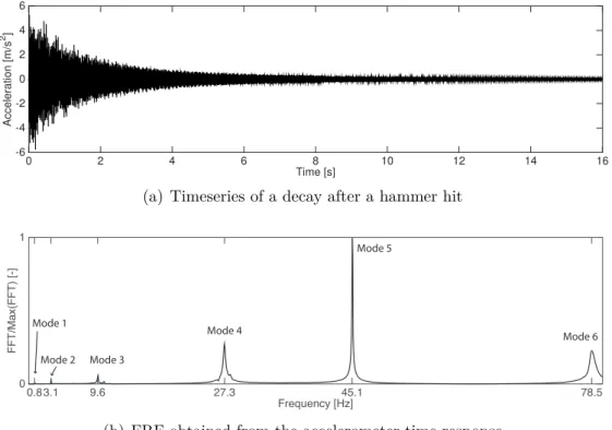
A roving hammer test was carried out to identify the first few linear modes of vibration of the structural system. The wing was impacted five times in 24 different locations using a hammer instrumented with a load cell. The response was measured with a single accelerometer placed on the trailing edge at the tip of the wing while the modal parameters were estimated from the Frequency Response Function (FRF) of the signal. Figure 2.6 depicts a typical system response and the corresponding FRF where six modes are clearly identified. Time [s] 0 2 4 6 8 10 12 14 16 Acceleration [m/s 2] -6 -4 -2 0 2 4 6
(a) Timeseries of a decay after a hammer hit
Frequency [Hz] 0.8 3.1 9.6 27.3 45.1 78.5 F F T /Ma x(F F T ) [-] 0 1 Mode 1 Mode 2 Mode 3 Mode 4 Mode 5 Mode 6
(b) FRF obtained from the accelerometer time response
Figure 2.6: Accelerometer time response and FRF used to perform linear wind-off modal analysis on the setup
Mode 1 Mode 2 Mode 3 Mode 4 Mode 5 Mode 6
Frequency [Hz] 0.84 3.1 9.6 27.3 45.1 78.5
Damping ratio [%] 0.84 0.24 0.40 0.35 0.06 0.39
2.3 Wind-off identification 31
Since it is very difficult to excite the leaf spring with the hammer, its modal shapes are estimated from a shell element model of the whole structure computed by means of the Finite Element package SAMCEF. The first six modes of the complete system are depicted in figure 2.7 and their frequencies and damping ratios, identified using the Half-Power method, are given in table 2.1. The system’s modes of vibration can be described as follows:
1. Mode 1: first flexural mode of the leaf spring and no deformation of the flat plate. It is dominated by –, the flap DOF of the Hancock wing. The response of all three sensors should be in phase when this mode is excited.
2. Mode 2: first torsional mode of the leaf spring and no deformation of the flat plate. It mostly involves ◊, the pitch DOF of the Hancock Wing. The response of sensors 1-2 should be in phase while the response of sensors 1-3 and 2-3 should be out of phase when this mode is excited.
3. Mode 3: second flexural mode of the leaf spring and first flexural mode of the flat plate. The response of all the sensors should be in phase when this mode is excited but, in contrast to the flap mode case, sensor 1 should measure larger accelerations/displacements than sensor 2. The effect of the deflection of the wing is so small compared to that of the deflection of the leaf spring that this mode could be approximated by a rigid plate with a combination of a flap DOF and a plunge DOF.
4. Mode 4: second flexural mode of the leaf spring and second flexural mode of the flat plate. The response of sensors 2-3 should be in phase while that of sensors 1-2 and 1-3 should be out of phase.
5. Mode 5: first torsional mode of the flat plate. It is not possible to differentiate this mode from mode 4 with the sensor setup used in this study.
6. Mode 6: second flexural mode of the leaf spring and third flexural mode of the flat plate.
Considering the mode shapes, the pitch angle defined in section 2.2 is mostly due to mode 2, which is the only one that leads to significant relative displacement between sensors 2 and 3. Conversely, the flap angle can be a combination of the displacements of modes 1, 3, 4, 5 and 6 and great care should be taken when comparing this angle to the predictions of the model of the Hancock wing, which only represents mode 1.
Mode n° 1: F = 0.9 Hz Mode n° 2: F = 3.1 Hz Mode n° 3: F = 9.6 Hz
Mode n° 4: F = 27.3 Hz Mode n° 5: F = 45.1 Hz Mode n° 6: F = 78.5 Hz
Figure 2.7: First six mode shapes of the NLPFW. The squares indicate the positions of sensors A1 & D1, the circles A2 & D2 and triangles A3 & D3. The crossed circle
indicates the position of the accelerometer used for the roving hammer test.
2.3.2 Nonlinear identification
Nonlinear identification was performed on the flap and pitch modes using large amplitude free-decay tests in order to measure the frequency and damping amplitude dependence of the pitch and flap modes.
Figure 2.8 plots the response of the flap DOF after an initial condition –0 ¥ 10 deg
and the Wavelet Transform [111] of the response, which indicates the response frequency variation with time. Despite the large amplitude variation during the decay, the frequency remains approximately constant, which suggests that the stiffness in flap is linear in the displacement range considered.
Figure 2.9 depicts the response of the pitch after an initial condition ◊0 ¥ 6 deg and
the Wavelet Transform of the response. This time, the frequency of the oscillations is initially close to 4 Hz and decreases smoothly to 3.09 Hz, the linear frequency of the pitch mode, as the amplitude of the motion is reduced. This response is typical of a system with hardening stiffness.
Relating the frequency of the modes to the oscillation amplitude yields the frequency backbones of the nonlinear modes. Figure 2.10(a) plots the flap and pitch frequency backbones of the system computed from the time series of figures 2.8(a) & 2.9(a). The black markers are obtained by computing the amplitude and the instantaneous frequency