Addressing the determinants of built-up expansion and densification processes at the regional scale

1

Addressing the determinants of built-up expansion

and densification processes at the regional scale

Ahmed Mustafa1,*_{, Anton Van Rompaey², Mario Cools}1_{, Ismaïl Saadi}1_{, Jacques Teller}1 1_{Liège University, Belgium, ²KU Leuven, Belgium}

*a.mustafa@uliege.be

The accepted (preprint) version, which is identical to the published version. https://doi.org/10.1177/0042098017749176

Abstract:

An in-depth understanding of the main factors behind built-up development is a key prerequisite for designing policies dedicated to a more efficient land use. Infill development policies are essential to curb sprawl and allow a progressive recycling of low-density areas inherited from the past. This paper examines the controlling factors of built-up expansion and densification processes in Wallonia (Belgium). Unlike the usual urban/built-up expansion studies, our approach considers various levels of built-up densities to distinguish between different types of developments, ranging from low-density extensions (or sprawl) to high-density infill development. Belgian cadastral data for 1990, 2000, and 2010 were used to generate four classes of built-up areas, namely, non-, low-, medium- and high-density areas. A number of socioeconomic, geographic, and political factors related to built-up development were operationalized following the literature. We then used a multinomial logistic regression model to analyze the effects of these factors on the transitions between different densities in the two decades between 1990 and 2010. The findings indicate that all the controlling factors show distinctive variations based on density. More specifically, the centrality of zoning policies in explaining expansion processes is highlighted. This is especially

2 the case for high-density expansions. In contrast, physical and neighborhood factors play a larger

role in infill development, especially for dense infill development.

Keywords: built-up expansion, infill development, built-up development controlling factors, multinomial logistic regression, regional scale.

3 1. Introduction

Urban sprawl is increasingly acknowledged as a significant environmental, economic, and social

challenge in both the USA (Nechyba and Walsh, 2004; Song and Zenou, 2006) and Europe (EEA, 2006; Hennig et al., 2015). Accordingly, policies have been developed to curb this phenomenon and foster a more efficient use of the land (Danielsen et al., 1999; Grant, 2009). Such policies are typically based on a combination of spatial planning with fiscal and economic measures, promoting infill development and land recycling. Infill development is expected to reduce the consumption of land and thereby lower the pressure on green and agricultural areas (Jehling et al., 2016; McConnell and Wiley, 2011). It

contributes to fostering urban development through the regeneration of vacant land and/or brownfields within cities (Loo et al., 2017) and to promoting a more efficient use of available amenities, such as roads, schools, retail areas, and public spaces (Burchell et al., 2000; Downs, 2001; Ooi and Le, 2013). Infill development is further expected to reduce traffic congestion through a more intensive use of public transport, especially when designed in a transit-oriented development perspective (Litman, 2016).

It should be stressed that infill development is not restricted to the reconversion of brownfields, even though it certainly has a role to play in this regard. Infill development is now increasingly targeting low- and medium-density urban areas, with significant densification capacities in terms of both available land and services. This is especially the case in countries like Belgium, where a number of built-up

neighborhoods are characterized by low density and some discontinuity with historical urban cores (EEA, 2011; Thomas et al., 2008; Marique et al., 2013). Indeed, Belgium in general and more

specifically Wallonia (the southern part of Belgium) are in a remarkable situation within the European context with regard to urban sprawl (Dujardin et al., 2012; EEA, 2011; Thomas et al., 2008). Hennig et al. (2015) measured urban sprawl trends for 32 European countries and reported that Belgium is one of

4 the countries most affected by sprawl.

Belgium is characterized by a mixed spatial planning style, which combines regulatory with

comprehensive planning dimensions (European Union, 1997). Land allocation is highly controlled by the regional zoning plan (plan de secteur) that covers the entire territory of the country. Dating back to the 1970s and 1980s, the zoning plan has long contributed to creating urban sprawl, as it dedicates large scattered zones to built-up uses throughout the country (Poelmans and Van Rompaey, 2009).

Furthermore, the spatial planning system in Belgium is characterized by weak vertical relationships between territorial levels (regions and municipalities) and weak horizontal relationships between actors at the same territorial level (ESPON, 2005).

The combination of these two elements—the role of an oversized zoning plan and the lack of

coordination between stakeholders—may somehow hinder infill development, even when land recycling and controlling sprawl are explicitly pursued by the spatial development strategies adopted in all three regions of the country.

A better understanding of the mechanisms underlying built-up development processes is essential to improve the efficiency of the spatial planning system. Spatial models that explore the factors that control built-up development and/or simulate future expected scenarios may provide valuable information in this respect (Poelmans and Van Rompaey, 2009).

The objective of this paper is to compare the controlling factors of built-up expansion with densification, which is an essential component of spatial policies that aim to tackle urban sprawl (Nabielek, 2012; Tachieva, 2010). Our key motivation is to identify potential spatial drivers of low-density development and densification. To this end, built-up development in Wallonia was analyzed from 1990 to 2010 based on datasets derived from cadastral data. A multinomial logistic regression (MNL) model was employed

5 to explore the relationship between expansion/densification and a set of socioeconomic, geographic, and spatial planning factors.

The paper proceeds as follows. Section 2 presents previous work in the domain of land-use change models, stressing the need for greater consideration of built-up densities within these models. Section 3 gives details about the study area (Wallonia), the MNL model, and data preparation. We report our results and discuss these in Section 4, with Section 5 presenting our conclusions.

2. Previous work on densification

Aguayo et al. (2007) identified three main elements for land-use change spatial models: (i) examining the factors that control the change (e.g., Liu and Ma, 2011; Shu et al., 2014); (ii) projecting future scenarios and their potential impacts (e.g., Mustafa et al., 2016; Robinson et al., 2012); and (iii)

evaluating the impacts of different spatial policies on land-use patterns (e.g., Guzy et al., 2008; Jantz et al., 2003). In line with the aims of this study, we focus on exploring the factors that control built-up development considering both expansion and densification processes.

A number of studies have aimed at a better understanding of built-up controlling factors. Oueslati et al. (2015) examine the relationship between urban sprawl and a set of controlling factors in several

European cities. Their results show the significant role that socioeconomic, transportation, and

environmental factors play in urban sprawl. Li et al. (2013), Nong and Du (2011), Shu et al. (2014), and Traore and Watanabe (2017) explore the historical effects of physical, socioeconomic, and

neighborhood factors on urban expansion in relation to different geographical locations. Braimoh and Onishi (2007) identify the factors underlying residential and industrial/commercial development in Lagos (Nigeria) between 1984 and 2000. The findings of these studies provide important implications

6 for spatial planning. In many studies, the relationship between controlling factors and built-up

development is analyzed with logistic regression (logit) models. These studies confirmed that logit models are empirically robust.

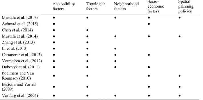
Typically, the identification of potential factors controlling built-up/urban expansion is based on expert knowledge of the specific study area as well as a literature review (Cammerer et al., 2013). The variety of controlling factors introduced in recent urban/built-up studies is summarized in Table 1. These factors can be grouped into five categories: (i) accessibility factors; (ii) topological factors; (iii) neighborhood factors; (iv) socioeconomic factors; and (v) spatial planning policies.

Table 1. Controlling factors of urban expansion considered in some recent studies. Accessibility

factors Topological factors Neighborhood factors

Socio-economic factors Spatial planning policies Mustafa et al. (2017) ● ● ● ● ● Achmad et al. (2015) ● ● Chen et al. (2014) ● ● Mustafa et al. (2014) ● ● ● ● ● Zhang et al. (2013) ● ● Li et al. (2013) ● ● ● Cammerer et al. (2013) ● ● ● ● Vermeiren et al. (2012) ● ● ● Dubovyk et al. (2011) ● ● ● ●

Poelmans and Van

Rompaey (2010) ● ● ● ●

Batisani and Yarnal

(2009) ● ● ● ●

Verburg et al. (2004) ● ● ● ● ●

Accessibility factors, such as distance to roads, are often taken into consideration in land-use change modeling (Aguayo et al., 2007). Herbert and Thomas (1982) claim that sprawl is commonly controlled by accessibility factors. A high accessibility level plays a decisive role in decreasing travel costs and making far-out land more accessible, resulting in lower-density urban developments. Topological

7 factors, such as elevation, are correlated with the price of urban development. Liu et al. (2016) suggest that the construction cost is considerably high for rugged lands.

Neighborhood factors, such as the proportion of urban land in the neighborhood, are especially

important because of the fact that built-up development can be regarded as a self-organizing system in which neighboring interaction strongly influences new developments (Poelmans and Van Rompaey, 2010). Many developers tend to develop land near to existing built-up areas because of the lower development risk for their investment (Rui and Ban, 2010). Socioeconomic factors, such as population density and employment potential, are quite often considered as active drivers of built-up development (Liu and Ma, 2011). For instance, economic activities may lead to a concentration of populations, which increases pressure on housing and housing prices in the center. Thus, it could be cheaper to develop land outside urban centers in areas characterized by lower density (Christiansen and Loftsgarden, 2011).

The influence of these controlling factors on built-up development is usually measured on regular grids composed of square cells of a dimension between 3030 m and 300300 m (e.g. Feng et al., 2011; Hao et al., 2013; Hu and Lo, 2007; Liu et al., 2008; Vermeiren et al., 2012). Most studies assume that built-up/urban expansion is a binary process, contrasting two classes of cells, i.e., built-up vs nonbuilt-up cells (e.g., Mustafa et al., 2017; Vermeiren et al., 2012). Such a binary representation of built-up environment somehow disregards the fuzzy nature of urban boundaries (Ban and Ahlqvist, 2009). More importantly, it tends to conceal the potential for further infill development within already built-up areas when their present density and level of services allow it. Some studies have specifically considered multiple urban densities (e.g. Mustafa et al., 2016, 2015; Xian and Crane, 2005; Yang, 2010). Considering various levels of densities is necessary to measure the influence of controlling factors on densification processes and infill development (Loibl and Toetzer, 2003; Tian et al., 2005); this is especially important as the

8 factors governing sprawl and infill development may not be identical in their nature or their relative importance. Eliciting these differences requires modeling both expansion and densification processes. Finally, measuring past densification processes and the factors behind these may help to reveal and activate available capacity in already built-up areas, which is in line with current land recycling policies.

In sum, a major difference in our approach compared with previous work is that we examine the

potential of the spatial models to explore the factors behind built-up development, considering different levels of density and the drivers of infill development.

3. Material and methods

3.1 Study area

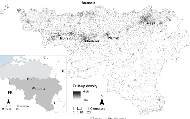
Wallonia (Figure 1) accounts for 55% of the territory of Belgium with a total area of 16,844 km2 _{– to}

give an idea, this area is slightly larger than Northern Ireland in the UK or the US state of Connecticut. Its main urban cores are Charleroi, Liège, Mons, and Namur, which are all characterized by a historical city center, around which the urban development has expanded. The total population of Wallonia in 2010 was 3,498,384 inhabitants, corresponding to one-third of the Belgium population (Belgian Federal Government, 2013). The population is mainly concentrated in the northern areas, following the

nineteenth-century industrial axis, running from east (Liège) to west (Mons) (Thomas et al., 2008). North of this axis, urban landscapes are highly influenced by the Brussels metropolitan area. Toward the far south of Wallonia, urban development is influenced by the presence of the city of Luxembourg (Thomas et al., 2008). Topographically, elevations in the region range from sea level to 693 m above sea level.

9 Figure 1: Study area.

Wallonia is characterized by a strong sprawl and the resulting landscape fragmentation (Dujardin et al., 2014; EEA, 2011). Densification strategies are especially important in such a context so as to limit the further consumption of land and to better structure existing peri-urban areas considering their

specificities (De Smet and Teller, 2016).

3.2 Outline of the model

The built-up density index is calculated per 1 ha (100100 m) over Wallonia using Belgian cadastral data. The range of density values is then subdivided into four classes (nonbuilt-up, low-, medium-, and high-density built-up areas) by means of the natural breaks technique (Jenks and Caspall, 1971). To understand the expansion and densification processes, the methodology is tailored to identify the controlling factors of (i) expansion of the three density classes vs the nonbuilt-up class, and (ii) transitions from low- and medium-density classes to medium- and high-density classes.

10 We employ a multinomial logistic regression (MNL) model to examine the relationship between

expansion/densification and their controlling factors. The MNL model allows for the consideration of several classes as the dependent variable (Yn), using a set of independent explanatory variables (Xs). When working with MNL models, three kinds of dependent variables should be considered: (i) the nominal Y responses; (ii) the categorical responses with natural ordering; and (iii) the nested responses when one category is nested in the previous one. In this paper, the dependent variable for the model is initially treated as categorical under the assumption that the levels of dependent status have a natural ordering (i.e., low to high density). To evaluate this assumption, the test of the proportional odds assumption is performed. The significance of the chi-squared statistic of the test is <0.001, which implies that the assumption of having a natural ordering in the dependent variable is violated. We then employ a nested MNL model with two levels: (i) built-up vs nonbuilt-up densities; and (ii) three built-up densities. The inclusive values (IVs) for the two nested levels are 0.8 and 3.9. Since at least one of the IVs is outside the 0–1 range, we decided not to opt for the nested MNL, as the parameter estimates are only consistent with utility maximization for a certain value range of the explanatory variables (Ortúzar and Willumsen, 1994). Accordingly, a nominal MNL model is adopted for this study.

The general form of the MNL model can be represented as:

1 11 1 12 2 1 1 1 2 2 1 ... ... log( ) ... log( ) _{n n n n} k k k k v k k k k v v n v X X X X X X k k                   (1)

where log(kn) is the natural logarithm of class kn vs the reference class k0, X is a set of explanatory variables (X1, X2,…, Xv), 𝛼_𝑘𝑛 is the intercept term for class kn vs the reference class, and 𝛽is the slopes for the classes (the coefficient vector). Thus, the probabilities of each class can be obtained using the following formula:

11

 

 





 





1 exp(log( )) exp(log( )) ... exp(log( )) exp

,

1 exp(log( )) exp(log( )) ... exp(log( )) exp

,

1 exp(log( )) exp(log( )) ... exp(log( ))

( ) log( ) ( ) ... log( ) ( ) n n n n n c ij c ij c ij Y k k k k k Y k k k k k Y k k k k P P P                   (2)

where ((Pc)ij,Y=kn) is the probability of change from the reference class to class kn occurring in cell ij. The MNL model employs the maximum likelihood estimation method to achieve the best-fit sets of coefficients for each X.

The model is performed for two observed periods, 1990–2000 and 2000–2010, using Belgian cadastral data. A comparison of the two periods allows the measurement of the stability of the role of the different factors over time. The MNL outcomes are a set of coefficients that define the contribution of each controlling factor to the built-up development, as well as a map of probability of being built-up for each class, which is generated by plugging the coefficients of the MNL model into Equation (2). The MNL model assesses overall model performance and the significance of individual X variables. The X

variables were selected by entry testing based on the significance of the score statistic (P-value), which was set to P0.05. Only variables significant at P0.05 on at least one class were included in the final MNL model.

The goodness-of-fit of the model runs was evaluated using the relative operating characteristic (ROC) method. The ROC is an excellent method to estimate the quality of a model that predicts the occurrence of an event by comparing a probability map depicting the likelihood of change occurring and a binary map showing where the changes actually occurred (Hu and Lo, 2007). A ROC value of 0.5 means completely random discrimination and 1 means perfect discrimination.

12

3.2.1 Dependent variables

The dependent variables for the MNL model are defined using the cadastral dataset (CAD). CAD is a vector dataset representing buildings in two dimensions as polygons, made available by the Land Registry Administration of Belgium. CAD provides the construction date for each building. This information was used to generate three built-up maps for 1990, 2000, and 2010. CAD vector data were then rasterized at a very fine cell dimension of 22 m.

One of the independent variables, elevation (DEM), is available at 1010 m cell size and therefore we should aggregate the rasterized CAD data to at least 1010 m (representing a building of 100 m). The computational time and resources required to process the 1010 m datasets, about 400,000,000 cells, are huge. Data aggregation can efficiently reduce the computational resources of our model. Still the

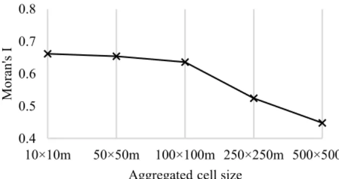
modifiable areal unit problem (MAUP) should be considered when aggregating spatial data (Openshaw, 1984; Openshaw and Taylor, 1979). To examine the effects of aggregation in the context of the MAUP, we performed a series of the first-lag autocorrelation analyses based on Moran’s I test following Jelinski and Wu (1996). The conceptualization of spatial relations is based on King’s (queens) case analysis, which considers a neighborhood window of eight cells. As a result of this sensitivity analysis (Figure 2), we selected an aggregated cell of 100100 m, which appears as the best combination between

aggregation dimension and Moran’s I. Moreover, the 100100 m cell size is commonly used in regional land use models (e.g. Mustafa et al., 2017; Poelmans and Van Rompaey, 2010).

13 Each aggregated cell has a density value that exhibits the number of 22 m cells located within its boundary. This density value will be used as a built-up density index for each aggregated 100100 m cell. The minimum density value adopted for considering 100100 m cells as built-up is 25. The

threshold of 25 (representing a building of 100 m2_{) corresponds to an average-sized residential building}

in Belgium (Tannier and Thomas, 2013). The density value is then used to represent four classes: (class-0) nonbuilt-up, (class-1) low-density, (class-2) medium-density, and (class-3) high-density built-up.

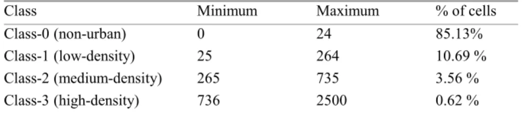
The natural breaks classification method was used to set the thresholds that define the different classes. This method effectively ensures a high internal homogeneity among classes (Fraile et al., 2016). The natural breaks method uses the Jenks optimization algorithm (Jenks and Caspall, 1971), which identifies breaks by the arrangement of classes that best groups similar values. This is done by minimizing the average deviation of each class from its mean and maximizing that average deviation from the means of the other classes. Table 2 presents the resulting thresholds, which define the different densities for the model implementation. The low-density and scattered built-up landscape of Wallonia resulted in low thresholds for medium and high densities.

0.4 0.5 0.6 0.7 0.8 10×10m 50×50m 100×100m 250×250m 500×500m M or an 's I

Aggregated cell size

Figure 2: Effects of data aggregation on spatial autocorrelation (Moran’s I) resulting from aggregation procedures for cadastral dataset.

14 Table 2. Range of built-up classes in the number of 22 cells.

Class Minimum Maximum % of cells

Class-0 (non-urban) 0 24 85.13%

Class-1 (low-density) 25 264 10.69 % Class-2 (medium-density) 265 735 3.56 % Class-3 (high-density) 736 2500 0.62 %

3.2.2 Built-up development controlling factors

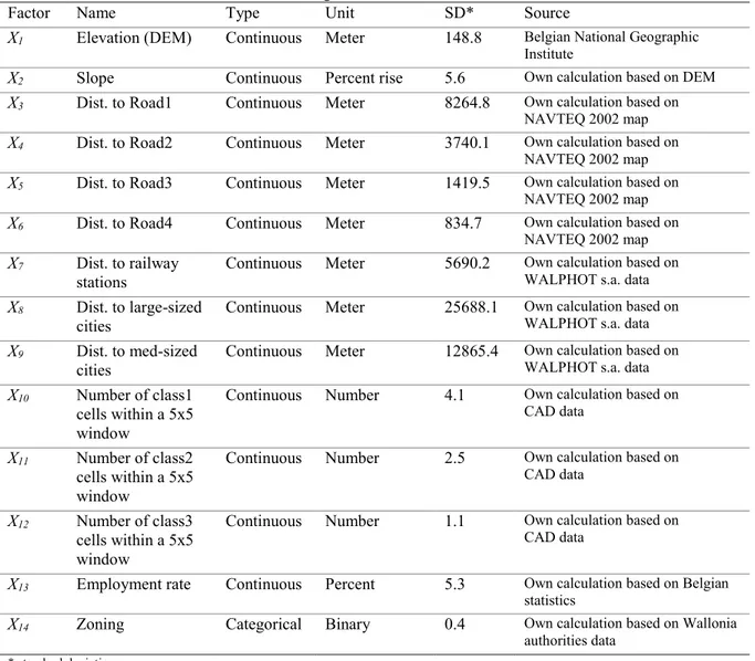
The accessibility factors included in this study are the Euclidian distance to Road1 (highways), Road2 (main roads), Road3 (secondary roads), Road4 (local roads), railway stations, large-sized Belgian cities (population >90,000), and medium-sized Belgian cities (population 20,000–90,000). For the topological factors, slope and elevation are included. Employment rate is considered as a socioeconomic factor. The number of existing built-up cells from each density class within a 55 cell neighborhood is included in this study to consider local interaction effects. The selection of the neighborhood size was made because previous studies found that the defined neighborhood using all surrounding cells within a radius of one to eight cells can capture the operational range of the local processes being modeled (e.g., Hu and Lo, 2007; Roy Chowdhury and Maithani, 2014). Table 3 gives the complete list of the selected controlling factors, Xs.

All data used in this study are represented as a 100100 m raster grid. X variables are measured in different units so we standardized all continuous X variables. If some X variables relatively measured the same phenomena, strong collinearities would cause an erroneous estimation of the MNL model’s

parameters. Consequently, a multicollinearity test was examined in the initial stage using variance inflation factors (VIF). Montgomery and Runger (2003) recommended that the VIFs should not exceed 4.

15 Table 3. List of selected urbanization controlling factors.

Factor Name Type Unit SD* Source

X1 Elevation (DEM) Continuous Meter 148.8 Belgian National Geographic

Institute

X2 Slope Continuous Percent rise 5.6 Own calculation based on DEM

X3 Dist. to Road1 Continuous Meter 8264.8 Own calculation based on

NAVTEQ 2002 map

X4 Dist. to Road2 Continuous Meter 3740.1 Own calculation based on

NAVTEQ 2002 map

X5 Dist. to Road3 Continuous Meter 1419.5 Own calculation based on

NAVTEQ 2002 map

X6 Dist. to Road4 Continuous Meter 834.7 Own calculation based on

NAVTEQ 2002 map

X7 Dist. to railway stations

Continuous Meter 5690.2 Own calculation based on WALPHOT s.a. data

X8 Dist. to large-sized

cities Continuous Meter 25688.1

Own calculation based on WALPHOT s.a. data

X9 Dist. to med-sized

cities Continuous Meter 12865.4

Own calculation based on WALPHOT s.a. data

X10 Number of class1 cells within a 5x5 window

Continuous Number 4.1 Own calculation based on CAD data

X11 Number of class2 cells within a 5x5 window

Continuous Number 2.5 Own calculation based on CAD data

X12 Number of class3 cells within a 5x5 window

Continuous Number 1.1 Own calculation based on CAD data

X13 Employment rate Continuous Percent 5.3 Own calculation based on Belgian

statistics

X14 Zoning Categorical Binary 0.4 Own calculation based on Wallonia

authorities data * standard deviation

X variables may exhibit spatial autocorrelation, which would bias the results of the regression analysis

(Overmars et al., 2003). To address this issue, logistic regression land-use models are commonly

calibrated based on a data sampling approach (e.g. Cammerer et al., 2013; Huang et al., 2010; Puertas et al., 2014). An alternative solution is the autologistic regression model, which considers an

autocorrelative term in the regression model. A number of studies have argued that autologistic models outperform logistic models (e.g., Lin et al., 2011; Shafizadeh-Moghadam and Helbich, 2015). In contrast, some authors (e.g., Dormann, 2007) have reported that the logistic regression model tends to outperform the autologistic model in terms of estimation of model parameters. However, comparison of

16 both modeling approaches (logistic vs autologistic) is beyond the scope of the present paper. Our model was calibrated through a data sampling approach, which is commonly used in land-use change

modeling. The selection of samples is based on 100 runs of the MNL model with different random samples. The best sample set, evaluated by ROC, was then selected.

4. Results and discussion

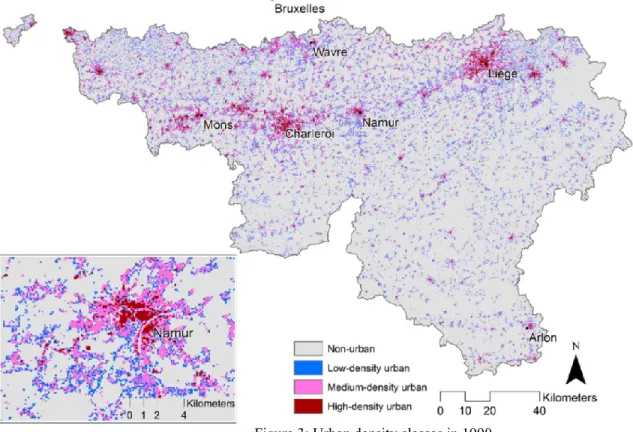
Figure 3 shows the spatial distribution pattern of density classes in 1990. High-density cells are concentrated in existing metropolises, whereas medium-density cells tend to be located in their surroundings and low-density lands are likely to be found in rural and remote locations.

Figure 3: Urban density classes in 1990.

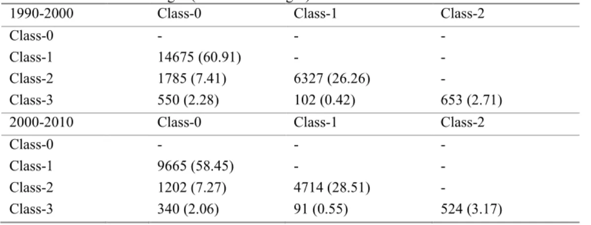
Table 4 summarizes class-to-class transitions from 1990 via 2000 to 2010. It can be seen that the

transition from nonbuilt-up to low-density developments (i.e., class-0 to class-1) largely dominates over both periods. However, a progressive trend toward infill development, namely densification of built-up

17 areas, can also be identified from this table. This trend should be amplified especially in the transitions from medium- to high-density developments (i.e., class-2 to class-3) in those areas that are best located in terms of accessibility to transport and services. This finding can be related to some recent spatial policies. Since 2005, the definition of a new zone to be urbanized in the regional zoning plan in Wallonia must be compensated by the downzoning of a similar-sized area that was to be urbanized beforehand to a nonurban zone (Prokop et al., 2011).

Table 4. Class-to-class changes (% of total changes).

1990-2000 Class-0 Class-1 Class-2

Class-0 - - -

Class-1 14675 (60.91) - -

Class-2 1785 (7.41) 6327 (26.26) -

Class-3 550 (2.28) 102 (0.42) 653 (2.71)

2000-2010 Class-0 Class-1 Class-2

Class-0 - - -

Class-1 9665 (58.45) - -

Class-2 1202 (7.27) 4714 (28.51) -

Class-3 340 (2.06) 91 (0.55) 524 (3.17)

Table 4 shows that the transitions from class-1 to class-3 over the study period are marginal. Thus, densification is considered as the transitions from class-1 to class-2 and from class-2 to class-3, whereas expansion is seen as the transitions from class-0 to classes 1–3.

The VIF test values (<1.59) for all standardized explanatory variables suggest that all X variables can be incorporated in the MNL model.

4.1 Built-up expansion

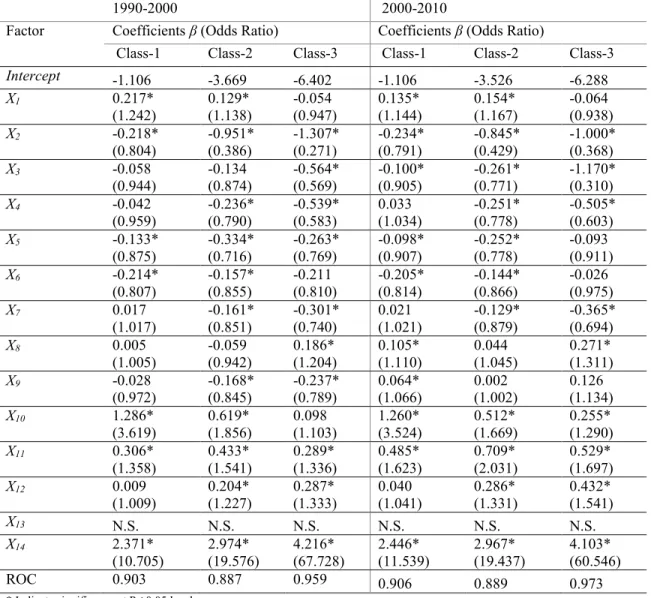
Table 5 presents the results of the expansion process, i.e., transitions from nonbuilt-up cells with a density of 0–24 to cells with built-up density classes 1–3. For the relative measurement of the contribution of each controlling factor to the expansion process, the odds ratio (OR), which equals

18

exp(), is calculated. An OR >1 (coefficients greater than 0) indicates a positive effect, i.e., the

probability of development increases with an increasing OR of the variable, whereas an OR <1 indicates a negative effect. The results indicate that the impact of the different controlling factors varies along with density.

Expansion of all density classes is highly correlated with zoning status (X14), which is in line with findings by Poelmans and Van Rompaey (2010). In both periods, the result shows a gradual upward trend in the zoning status from low density to high density. For instance, in 1990–2000, the expansion of classes 1, 2, and 3 is respectively around 11, 20, and 68 times more likely to be located in zones

designated for urban use than in zones designated for other land uses. To minimize administrative and financial risks, high-density developments are typically located in areas where the legally binding plan allows such developments. In contrast, built-up developments in areas adjacent to urban cores (medium density) such as suburbs do not strictly follow land use plans. The impact of zoning on transitions to low-density classes is lower than the one observed in other classes. Such transitions can be considered as remote areas, consisting of scattered buildings (1–3 buildings/ha), which can sometimes deviate from existing zoning plans, especially in agriculture-related zones.

In both periods, elevation (X1) is a positive determinant for low- and medium-density expansions, whereas slope (X2) has a remarkable negative effect on all expansion processes, as in Poelmans and Van Rompaey (2010), especially on the expansion of medium- and high-density classes. The model predicts that a 5.6% rise in slope decreases the odds of expansion by a factor of 0.4 for the medium-density class, and by 0.3 and 0.4 for the expansion of the high-density class in 1990–2000 and 2000–2010,

19 All statistically significant distances to road classes have OR values <1 implying that the closer to roads, the higher the expansion probability, as reported in Cammerer et al. (2013) and Poelmans and Van Rompaey (2010).

Table 5. The coefficients () of the MNL model for urban expansion (reference: class-0). Sample size 16,360.

1990-2000 2000-2010

Factor Coefficients β (Odds Ratio) Coefficients β (Odds Ratio)

Class-1 Class-2 Class-3 Class-1 Class-2 Class-3

Intercept _{-1.106 -3.669 -6.402 -1.106 -3.526 -6.288} X1 0.217* (1.242) 0.129* (1.138) -0.054 (0.947) 0.135* (1.144) 0.154* (1.167) -0.064 (0.938) X2 -0.218* (0.804) -0.951* (0.386) -1.307* (0.271) -0.234* (0.791) -0.845* (0.429) -1.000* (0.368) X3 -0.058 (0.944) -0.134 (0.874) -0.564* (0.569) -0.100* (0.905) -0.261* (0.771) -1.170* (0.310) X4 -0.042 (0.959) -0.236* (0.790) -0.539* (0.583) 0.033 (1.034) -0.251* (0.778) -0.505* (0.603) X5 -0.133* (0.875) -0.334* (0.716) -0.263* (0.769) -0.098* (0.907) -0.252* (0.778) -0.093 (0.911) X6 -0.214* (0.807) -0.157* (0.855) -0.211 (0.810) -0.205* (0.814) -0.144* (0.866) -0.026 (0.975) X7 0.017 (1.017) -0.161* (0.851) -0.301* (0.740) 0.021 (1.021) -0.129* (0.879) -0.365* (0.694) X8 0.005 (1.005) -0.059 (0.942) 0.186* (1.204) 0.105* (1.110) 0.044 (1.045) 0.271* (1.311) X9 -0.028 (0.972) -0.168* (0.845) -0.237* (0.789) 0.064* (1.066) 0.002 (1.002) 0.126 (1.134) X10 1.286* (3.619) 0.619* (1.856) 0.098 (1.103) 1.260* (3.524) 0.512* (1.669) 0.255* (1.290) X11 0.306* (1.358) 0.433* (1.541) 0.289* (1.336) 0.485* (1.623) 0.709* (2.031) 0.529* (1.697) X12 0.009 (1.009) 0.204* (1.227) 0.287* (1.333) 0.040 (1.041) 0.286* (1.331) 0.432* (1.541) X13 _{N.S. N.S. N.S. N.S. N.S. N.S.} X14 2.371* (10.705) 2.974* (19.576) 4.216* (67.728) 2.446* (11.539) 2.967* (19.437) 4.103* (60.546) ROC 0.903 0.887 0.959 _{0.906 0.889 0.973}

* Indicate significance at P≤ 0.05 level N.S. non-significant at P≤ 0.05 level

Distance to high-speed roads (X3 and X4) has a notable impact on the development of high-density areas, although it should be considered that a number of urban cores are directly accessible via high-speed roads in Wallonia. Distance to secondary roads (X5) contributes to the expansion of different density classes, especially the medium-density class, whereas distance to local roads (X6) has a remarkable

20 impact on the expansion of low-density areas in both periods, which is what can be expected, as many low-density areas are only accessible via local roads. The findings suggest that the new developments of medium- and high-density projects are likely to be located near train stations (X7) in 1990–2000 and 2000–2010.

Interpretation of the contribution of distance to large- and medium-sized cities (X8 and X9) in Wallonia indicates a decentralizing and suburbanizing trend over time. In 1990–2000, the impact of distance to large-sized cities positively affected high-density expansion. In 2000–2010, the distance to large-sized cities had a positive impact on low- and high-density classes. This means that the likelihood of low- and high-density developments increased with increasing distance to large-sized cities in both periods. In contrast, distance to medium-sized cities was a negative determinant of medium- and high-density expansion in 1990–2000 and remained positive on low-density expansion in 2000–2010.

The increasing number of existing low-density cells within a neighborhood of 55 size (X10) reveals a strong relationship with low-density expansion: every four low-density neighbors increase low-density expansion odds by around four times in 1990–2000 and 2000–2010. The probability of medium-density expansion is greater by increasing the number of existing low-, medium-, and high-density cells (X10,

X11, X12), whereas the probability of high-density expansion is greater by increasing the number of existing medium- and high-density cells (X11, X12) within a neighborhood. The lack of significant contribution of employment rate (X13) to the expansion processes indicates that it was not a limiting factor of the built-up expansion processes, as it was the case in Hu and Lo (2007) and Poelmans and Van Rompaey (2010).

21

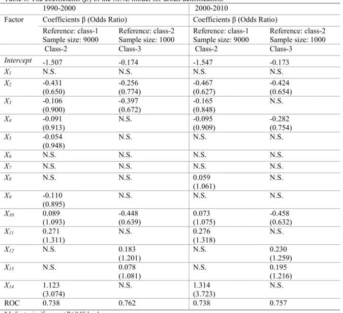
4.2 Built-up densification

Built-up densification is defined as transitions from low- to medium-density class, as well as transitions from medium- to high-density class. As such, it corresponds to infill development. In general, the magnitude of the unique effects of land-use policies (zoning) and accessibility factors declined along with the densification process. Table 6 lists the MNL model’s results of the densification process.

Table 6. The coefficients () of the MNL model for urban densification.

1990-2000 2000-2010

Factor Coefficients β (Odds Ratio) Coefficients β (Odds Ratio) Reference: class-1

Sample size: 9000 Reference: class-2 Sample size: 1000 Reference: class-1 Sample size: 9000 Reference: class-2 Sample size: 1000

Class-2 Class-3 Class-2 Class-3

Intercept -1.507 -0.174 -1.547 -0.173 X1 N.S. N.S. N.S. N.S. X2 -0.431 (0.650) -0.256 (0.774) -0.467 (0.627) -0.424 (0.654) X3 -0.106 (0.900) -0.397 (0.672) -0.165 (0.848) N.S. X4 -0.091 (0.913) N.S. -0.095 (0.909) -0.282 (0.754) X5 -0.054 (0.948) N.S. N.S. N.S. X6 N.S. N.S. N.S. N.S. X7 N.S. N.S. N.S. N.S. X8 N.S. N.S. 0.059 (1.061) N.S. X9 -0.110 (0.895) N.S. N.S. N.S. X10 0.089 (1.093) -0.448 (0.639) 0.073 (1.075) -0.458 (0.632) X11 0.271 (1.311) N.S. 0.276 (1.318) N.S. X12 N.S. 0.183 (1.201) N.S. 0.230 (1.259) X13 N.S. 0.078 (1.081) N.S. 0.195 (1.216) X14 1.123 (3.074) N.S. 1.314 (3.723) N.S. ROC 0.738 0.762 0.738 0.757

* Indicate significance at P≤ 0.05 level N.S. non-significant at P≤ 0.05 level

22 lower to higher densities tends to occur in flat areas. The estimated coefficients of slope in both periods highlight that slope—the only variable that has a statistically significant impact on all built-up

development processes—continues to play an important role in explaining both expansion and densification processes, compared with other variables in our model. When considering infill development policies, it could be expected that some variables, such as distance to train stations or accessibility to employment areas, would play a more significant role in driving urban development, by contributing to reducing home-to-work distances and increasing the use of sustainable modes of

transport. Our results indicate that in Wallonia this is not yet the case; urban development processes continue to be determined by physical factors, i.e., low slope areas that are scattered across the entire region.

Distance to high-speed roads (X3 and X4) negatively contributes to all densification processes. Other distance-related factors have no impact except for secondary roads, which contributed to the

densification of low-density areas in 1990–2000, and distance to large-sized cities, which contributed to the densification of low-density areas in 2000–2010.

Neighborhood plays a significant role in densification processes. In both periods, the odds of conversion of low-density lands into medium density are increased by a factor of 1.1 for every four low-density neighbors. Each medium-density neighbor increases the odds of low-density densification by ~0.5 times. The odds of conversion of medium density into high density are increased by ~1.2 for each high-density neighbor.

These findings suggest that existing high-density locations will generally experience a higher densification rate. Unlike the expansion processes, where the employment rate is not significant, the employment rate (X13) contributes positively to the densification of medium-density areas. However, the

23 contribution of this variable to the densification process is small compared with the other variables. The nonsignificant role of employment rate could be explained by the fact that many commuters (even car users) can deduct their transport costs from their income tax (De Decker, 2008). Together with the density of the road network, this may encourage people to choose to live in low-density settlements far from their workplaces.

Interestingly, the magnitude of the zoning status effect (X14) on the densification process decreases compared with the expansion process. The effect of zoning status on the change from medium- to high-density class is not significant. It also shows a moderate effect on the change from low to medium density in both periods.

The ROC values differ between the distinct processes of built-up development. The expansion process shows a relatively high goodness-of-fit with ROC values of 0.89–0.97. Estimation of the potential urban densification process produced many false-positives, which were estimated at ROC values of 0.74–0.76. This implies that the densification process is less predictable than the urban expansion process, which can be explained by the fact that most of the selected controlling factors were not statistically

significant. The ROC values for 1990–2000 and 2000–2010 were almost identical, indicating that there were no major changes in the built-up development trend over the study period.

5. Conclusions

Using a multinomial logistic regression model, this study explores the relationship between built-up expansion/densification and their controlling factors. It considers the three classes of built-up densities of low, medium, and high density. Previous built-up expansion models assumed a binary process of expansion, i.e., built-up vs nonbuilt-up. Tables 5 and 6 show that the assumption of a binary approach

24 may lead to inaccurate conclusions as the relative importance of the controlling factors typically varies with density, for both expansion and densification processes.

This study highlights significant factors that control low-density development, which is one of the main characteristics of urban sprawl. Spatial planning, road accessibility, and neighborhood interactions are important determinants of the low- and medium-density developments in Wallonia, Belgium. This finding is in line with those of other studies conducted in other regions of the world (e.g. Aguayo et al., 2007; Hu and Lo, 2007).

Our results indicate that there is a progressive shift from expansion to densification in Wallonia even though expansion processes remain very active. The densification processes show a nonsignificant relationship with railway stations, which means that infill development does not yet follow a transit-oriented development approach that would foster high-density developments around train stations. Proximity to medium- and large-sized cities does not appear to be a key factor in densification processes, even though it is certainly where infill development is most expected in terms of both real estate value and contribution to sustainable development. This phenomenon may be related to the fact that densification appears highly correlated with neighborhood characteristics, which may conceal the effect of proximity to medium- and large-sized cities where denser neighborhoods may be expected.

Our study reveals that infill development is mainly driven by local factors in Wallonia and that

expansion remains controlled by the zoning plan. In contrast, the influence of zoning on densification is not major. Infill development does not obey an official spatial policy adopted at the regional level that is articulated along clear sustainability principles. Hence, the impact of zoning on expansion and

densification appears counterproductive in some respects, which is quite unsatisfactory in terms of land-use policy. It should be stressed that zoning documents were drawn up in the 1970s and 1980s in

25 Wallonia, well before the current sustainability agenda. Even though these documents have been

partially revised since then, areas open to urban development remain overabundant in some parts of the region. A mechanism for the transfer of development rights should be designed to better allocate urban zones to places/nodes where infill development can be supported. At the same time, streamlining the modification of land-use plans and planning permission procedures in selected areas of the region may provide appropriate support for those processes.

The results of this study emphasize that the MNL model incorporating various classes of built-up densities provides useful information for policy makers who want to explore the relationships between spatial drivers of infill development. Contrasting the drivers underlying expansion and densification processes is essential for designing spatial policies that support improved land recycling and infill development.

Acknowledgments The research was funded by the ARC grant for Concerted Research Actions for project number 13/17-01 entitled “Land-use change and future flood risk: influence of micro-scale spatial patterns (FloodLand)”.

References

Achmad, A., Hasyim, S., Dahlan, B., Aulia, D.N., 2015. Modeling of urban growth in tsunami-prone city using logistic regression: Analysis of Banda Aceh, Indonesia. Appl. Geogr. 62, 237–246. doi:10.1016/j.apgeog.2015.05.001 Aguayo, M., Wiegand, T., Azócar, G., Wiegand, K., Vega, C., 2007. Revealing the Driving Forces of Mid-Cities Urban

Growth Patterns Using Spatial Modeling: a Case Study of Los Ángeles, Chile. Ecol. Soc. 12. doi:10.5751/ES-01970-120113

Ban, H., Ahlqvist, O., 2009. Representing and negotiating uncertain geospatial concepts – Where are the exurban areas? Comput. Environ. Urban Syst. 33, 233–246. doi:10.1016/j.compenvurbsys.2008.10.001

Batisani, N., Yarnal, B., 2009. Urban expansion in Centre County, Pennsylvania: Spatial dynamics and landscape transformations. Appl. Geogr. 29, 235–249. doi:10.1016/j.apgeog.2008.08.007

Belgian Federal Government, 2013. Statistics Belgium [WWW Document]. Stat. Belg. URL http://statbel.fgov.be/fr/statistiques/chiffres/ (accessed 4.29.14).

Braimoh, A.K., Onishi, T., 2007. Spatial determinants of urban land use change in Lagos, Nigeria. Land Use Policy 24, 502– 515. doi:10.1016/j.landusepol.2006.09.001

Burchell, R.W., Listokin, D., Galley, C.C., 2000. Smart growth: More than a ghost of urban policy past, less than a bold new horizon. Hous. Policy Debate 11, 821–879. doi:10.1080/10511482.2000.9521390

26 Cammerer, H., Thieken, A.H., Verburg, P.H., 2013. Spatio-temporal dynamics in the flood exposure due to land use changes

in the Alpine Lech Valley in Tyrol (Austria). Nat. Hazards 68, 1243–1270. doi:10.1007/s11069-012-0280-8 Chen, Y., Li, X., Liu, X., Ai, B., 2014. Modeling urban land-use dynamics in a fast developing city using the modified

logistic cellular automaton with a patch-based simulation strategy. Int. J. Geogr. Inf. Sci. 28, 234–255. doi:10.1080/13658816.2013.831868

Christiansen, P., Loftsgarden, T., 2011. Drivers behind urban sprawl in Europe. TØI Rep. 1136, 2011.

Danielsen, K.A., Lang, R.E., Fulton, W., 1999. Retracting suburbia: Smart growth and the future of housing. Hous. Policy Debate 10, 513–540. doi:10.1080/10511482.1999.9521341

De Decker, P., 2008. Facets of housing and housing policies in Belgium. J. Hous. Built Environ. 23, 155–171. doi:10.1007/s10901-008-9110-4

De Smet, F., Teller, J., 2016. Characterising the Morphology of Suburban Settlements: A Method Based on a Semi-automatic Classification of Building Clusters. Landsc. Res. 41, 113–130. doi:10.1080/01426397.2015.1045464

Dormann, C.F., 2007. Assessing the validity of autologistic regression. Ecol. Model. 207, 234–242. doi:10.1016/j.ecolmodel.2007.05.002

Downs, A., 2001. What does smart growth really mean. Planning 67, 20–25.

Dubovyk, O., Sliuzas, R., Flacke, J., 2011. Spatio-temporal modelling of informal settlement development in Sancaktepe district, Istanbul, Turkey. ISPRS J. Photogramm. Remote Sens., Quality, Scale and Analysis Aspects of Urban City Models 66, 235–246. doi:10.1016/j.isprsjprs.2010.10.002

Dujardin, S., Marique, A.-F., Teller, J., 2014. Spatial planning as a driver of change in mobility and residential energy consumption. Energy Build. 68, 779–785. doi:10.1016/j.enbuild.2012.10.059

Dujardin, S., Pirart, F., Brévers, F., Marique, A.-F., Teller, J., 2012. Home-to-work commuting, urban form and potential energy savings: A local scale approach to regional statistics. Transp. Res. Part Policy Pract. 46, 1054–1065.

doi:10.1016/j.tra.2012.04.010

EEA, 2011. Landscape fragmentation in Europe (Publication). European Environment Agency. EEA, 2006. Urban sprawl in Europe - The ignored challenge [WWW Document]. URL

http://www.eea.europa.eu/publications/eea_report_2006_10 (accessed 8.28.15).

ESPON, 2005. Governance of territorial and urban policies (No. 2nd Interim Report), ESPON Project 2.3.2. European spatial planning observation network.

European Union, 1997. The EU compendium of spatial planning systems and policies.

Feng, Y., Liu, Y., Tong, X., Liu, M., Deng, S., 2011. Modeling dynamic urban growth using cellular automata and particle swarm optimization rules. Landsc. Urban Plan. 102, 188–196. doi:10.1016/j.landurbplan.2011.04.004

Fraile, A., Larrodé, E., Alberto Magreñán, Á., Sicilia, J.A., 2016. Decision model for siting transport and logistic facilities in urban environments: A methodological approach. J. Comput. Appl. Math., Mathematical Modeling and Computational Methods 291, 478–487. doi:10.1016/j.cam.2014.12.012

Grant, J.L., 2009. Theory and Practice in Planning the Suburbs: Challenges to Implementing New Urbanism, Smart Growth, and Sustainability Principles. Plan. Theory Pract. 10, 11–33. doi:10.1080/14649350802661683

Guzy, M., Smith, C., Bolte, J., Hulse, D., Gregory, S., 2008. Policy Research Using Agent-Based Modeling to Assess Future Impacts of Urban Expansion into Farmlands and Forests. Ecol. Soc. 13. doi:10.5751/ES-02388-130137

Hao, P., Hooimeijer, P., Sliuzas, R., Geertman, S., 2013. What Drives the Spatial Development of Urban Villages in China? Urban Stud. 50, 3394–3411. doi:10.1177/0042098013484534

Hennig, E.I., Schwick, C., Soukup, T., Orlitová, E., Kienast, F., Jaeger, J.A.G., 2015. Multi-scale analysis of urban sprawl in Europe: Towards a European de-sprawling strategy. Land Use Policy 49, 483–498.

doi:10.1016/j.landusepol.2015.08.001

Herbert, D.T., Thomas, C.J., 1982. Urban Geography: A First Approach. Wiley.

Hu, Z., Lo, C.P., 2007. Modeling urban growth in Atlanta using logistic regression. Comput. Environ. Urban Syst. 31, 667– 688. doi:10.1016/j.compenvurbsys.2006.11.001

Huang, B., Xie, C., Tay, R., 2010. Support vector machines for urban growth modeling. GeoInformatica 14, 83–99. doi:10.1007/s10707-009-0077-4

Jantz, C.A., Goetz, S.J., Shelley, M.K., 2003. Using the Sleuth Urban Growth Model to Simulate the Impacts of Future Policy Scenarios on Urban Land Use in the Baltimore-Washington Metropolitan Area. Environ. Plan. B Plan. Des. 31, 251–271. doi:10.1068/b2983

Jehling, M., Hecht, R., Herold, H., 2016. Assessing urban containment policies within a suburban context—An approach to enable a regional perspective. Land Use Policy. doi:10.1016/j.landusepol.2016.10.031

Jelinski, D.E., Wu, J., 1996. The modifiable areal unit problem and implications for landscape ecology. Landsc. Ecol. 11, 129–140. doi:10.1007/BF02447512

27 Jenks, G.F., Caspall, F.C., 1971. Error on Choroplethic Maps: Definition, Measurement, Reduction. Ann. Assoc. Am. Geogr.

61, 217–244. doi:10.1111/j.1467-8306.1971.tb00779.x

Li, X., Zhou, W., Ouyang, Z., 2013. Forty years of urban expansion in Beijing: What is the relative importance of physical, socioeconomic, and neighborhood factors? Appl. Geogr. 38, 1–10. doi:10.1016/j.apgeog.2012.11.004

Lin, Y.-P., Chu, H.-J., Wu, C.-F., Verburg, P.H., 2011. Predictive ability of logistic regression, auto-logistic regression and neural network models in empirical land-use change modeling – a case study. Int. J. Geogr. Inf. Sci. 25, 65–87. doi:10.1080/13658811003752332

Litman, T., 2016. Evaluating Transportation Land Use Impacts: Considering the Impacts, Benefits and Costs of Different Land Use Development Patterns.

Liu, C., Ma, X., 2011. Analysis to driving forces of land use change in Lu’an mining area. Trans. Nonferrous Met. Soc. China 21, Supplement 3, s727–s732. doi:10.1016/S1003-6326(12)61670-7

Liu, X., Li, X., Shi, X., Wu, S., Liu, T., 2008. Simulating complex urban development using kernel-based non-linear cellular automata. Ecol. Model. 211, 169–181. doi:10.1016/j.ecolmodel.2007.08.024

Liu, Yaolin, He, Q., Tan, R., Liu, Yanfang, Yin, C., 2016. Modeling different urban growth patterns based on the evolution of urban form: A case study from Huangpi, Central China. Appl. Geogr. 66, 109–118. doi:10.1016/j.apgeog.2015.11.012 Loibl, W., Toetzer, T., 2003. Modeling growth and densification processes in suburban regions—simulation of landscape

transition with spatial agents. Environ. Model. Softw., Applying Computer Research to Environmental Problems 18, 553–563. doi:10.1016/S1364-8152(03)00030-6

Loo, B.P.Y., Cheng, A.H.T., Nichols, S.L., 2017. Transit-oriented development on greenfield versus infill sites: Some lessons from Hong Kong. Landsc. Urban Plan. 167, 37–48. doi:10.1016/j.landurbplan.2017.05.013

Marique, A.-F., Dujardin, S., Teller, J., Reiter, S., 2013. Urban sprawl, commuting and travel energy consumption. Proc. Inst. Civ. Eng. Energy 166. doi:10.1680/ener.12.00002

McConnell, V., Wiley, K., 2011. Infill Development: Perspectives and Evidence from Economics and Planning. doi:10.1093/oxfordhb/9780195380620.013.0022

Montgomery, D.C., Runger, G.C., 2003. Applied Statistics and Probability for Engineers, Fourth. ed. John Wiley & Sons, New York.

Mustafa, A., Bruwier, M., Teller, J., Archambeau, P., Erpicum, S., Pirotton, M., Dewals, B., 2016. Impacts of urban expansion on future flood damage: A case study in the River Meuse basin, Belgium, in: Sustainable Hydraulics in the Era of Global Change. Taylor & Francis Group.

Mustafa, A., Cools, M., Saadi, I., Teller, J., 2017. Coupling agent-based, cellular automata and logistic regression into a hybrid urban expansion model (HUEM). Land Use Policy 69C, 529–540. doi:10.1016/j.landusepol.2017.10.009 Mustafa, A., Cools, M., Saadi, I., Teller, J., 2015. Urban Development as a Continuum: A Multinomial Logistic Regression

Approach, in: Gervasi, O., Murgante, B., Misra, S., Gavrilova, M.L., Rocha, A.M.A.C., Torre, C., Taniar, D., Apduhan, B.O. (Eds.), Computational Science and Its Applications -- ICCSA 2015, Lecture Notes in Computer Science. Springer International Publishing, pp. 729–744.

Mustafa, A., Saadi, I., Cools, M., Teller, J., 2014. Measuring the Effect of Stochastic Perturbation Component in Cellular Automata Urban Growth Model. Procedia Environ. Sci., 12th International Conference on Design and Decision Support Systems in Architecture and Urban Planning, DDSS 2014 22, 156–168. doi:10.1016/j.proenv.2014.11.016

Nabielek, K., 2012. The Compact City: Planning strategies, recent developments and future prospects in the Netherlands - PBL Netherlands Environmental Assessment Agency, in: Proceedings of the AESOP 26th Annual Congress. Presented at the AESOP 26th Annual Congress, Ankara.

Nechyba, T.J., Walsh, R.P., 2004. Urban Sprawl. J. Econ. Perspect. 18, 177–200. doi:10.1257/0895330042632681 Nong, Y., Du, Q., 2011. Urban growth pattern modeling using logistic regression. Geo-Spat. Inf. Sci. 14, 62–67.

doi:10.1007/s11806-011-0427-x

Ooi, J.T.L., Le, T.T.T., 2013. The spillover effects of infill developments on local housing prices. Reg. Sci. Urban Econ. 43, 850–861. doi:10.1016/j.regsciurbeco.2013.08.002

Openshaw, S., 1984. The modifiable areal unit problem. Presented at the CATMOG 38, Geo Abstracts University of East Anglia.

Openshaw, S., Taylor, P.J., 1979. A million or so correlation coefficients: three experiments on the modifiable areal unit problem. Stat. Appl. Spat. Sci. 21, 127–144.

Ortúzar, J. de D., Willumsen, L.G., 1994. Modelling Transport, Second. ed. Wiley.

Oueslati, W., Alvanides, S., Garrod, G., 2015. Determinants of urban sprawl in European cities. Urban Stud. 0042098015577773. doi:10.1177/0042098015577773

Overmars, K.P., de Koning, G.H.J., Veldkamp, A., 2003. Spatial autocorrelation in multi-scale land use models. Ecol. Model. 164, 257–270. doi:10.1016/S0304-3800(03)00070-X

28 Poelmans, L., Van Rompaey, A., 2010. Complexity and performance of urban expansion models. Comput. Environ. Urban

Syst. 34, 17–27. doi:10.1016/j.compenvurbsys.2009.06.001

Poelmans, L., Van Rompaey, A., 2009. Detecting and modelling spatial patterns of urban sprawl in highly fragmented areas: A case study in the Flanders–Brussels region. Landsc. Urban Plan. 93, 10–19. doi:10.1016/j.landurbplan.2009.05.018 Prokop, G., Jobstmann, H., Schönbauer, A., 2011. Best practices for limiting soil sealing and mitigating its effects (Technical

Report No. 2011-050). European Commission – DG Environment.

Puertas, O.L., Henríquez, C., Meza, F.J., 2014. Assessing spatial dynamics of urban growth using an integrated land use model. Application in Santiago Metropolitan Area, 2010–2045. Land Use Policy 38, 415–425.

doi:10.1016/j.landusepol.2013.11.024

Robinson, D.T., Murray-Rust, D., Rieser, V., Milicic, V., Rounsevell, M., 2012. Modelling the impacts of land system dynamics on human well-being: Using an agent-based approach to cope with data limitations in Koper, Slovenia. Comput. Environ. Urban Syst., Special Issue: Geoinformatics 2010 36, 164–176.

doi:10.1016/j.compenvurbsys.2011.10.002

Roy Chowdhury, P.K., Maithani, S., 2014. Modelling urban growth in the Indo-Gangetic plain using nighttime OLS data and cellular automata. Int. J. Appl. Earth Obs. Geoinformation 33, 155–165. doi:10.1016/j.jag.2014.04.009

Rui, Y., Ban, Y., 2010. Multi-agent Simulation for Modeling Urban Sprawl In the Greater Toronto Area, in: 13th AGILE. Presented at the 13th International Conference on Geographic Information Science 2010, Portugal.

Shafizadeh-Moghadam, H., Helbich, M., 2015. Spatiotemporal variability of urban growth factors: A global and local perspective on the megacity of Mumbai. Int. J. Appl. Earth Obs. Geoinformation 35, Part B, 187–198.

doi:10.1016/j.jag.2014.08.013

Shu, B., Zhang, H., Li, Y., Qu, Y., Chen, L., 2014. Spatiotemporal variation analysis of driving forces of urban land spatial expansion using logistic regression: A case study of port towns in Taicang City, China. Habitat Int. 43, 181–190. doi:10.1016/j.habitatint.2014.02.004

Song, Y., Zenou, Y., 2006. Property tax and urban sprawl: Theory and implications for US cities. J. Urban Econ. 60, 519– 534. doi:10.1016/j.jue.2006.05.001

Tachieva, G., 2010. Sprawl Repair Manual, 2 edition. ed. Island Press, Washington.

Tannier, C., Thomas, I., 2013. Defining and characterizing urban boundaries: A fractal analysis of theoretical cities and Belgian cities. Comput. Environ. Urban Syst. 41, 234–248. doi:10.1016/j.compenvurbsys.2013.07.003

Thomas, I., Frankhauser, P., Biernacki, C., 2008. The morphology of built-up landscapes in Wallonia (Belgium): A classification using fractal indices. Landsc. Urban Plan. 84, 99–115. doi:10.1016/j.landurbplan.2007.07.002

Traore, A., Watanabe, T., 2017. Modeling Determinants of Urban Growth in Conakry, Guinea: A Spatial Logistic Approach. Urban Sci. 1, 12. doi:10.3390/urbansci1020012

Verburg, P.H., van Eck, J.R.R., de Nijs, T.C.M., Dijst, M.J., Schot, P., 2004. Determinants of Land-Use Change Patterns in the Netherlands. Environ. Plan. B Plan. Des. 31, 125–150. doi:10.1068/b307

Vermeiren, K., Van Rompaey, A., Loopmans, M., Serwajja, E., Mukwaya, P., 2012. Urban growth of Kampala, Uganda: Pattern analysis and scenario development. Landsc. Urban Plan. 106, 199–206. doi:10.1016/j.landurbplan.2012.03.006 Xian, G., Crane, M., 2005. Assessments of urban growth in the Tampa Bay watershed using remote sensing data. Remote

Sens. Environ. 97, 203–215. doi:10.1016/j.rse.2005.04.017

Yang, X., 2010. Integration of Remote Sensing with GIS for Urban Growth Characterization, in: Jiang, B., Yao, X. (Eds.), Geospatial Analysis and Modelling of Urban Structure and Dynamics, GeoJournal Library. Springer Netherlands, pp. 223–250. doi:10.1007/978-90-481-8572-6_12

Zhang, Z., Su, S., Xiao, R., Jiang, D., Wu, J., 2013. Identifying determinants of urban growth from a multi-scale perspective: A case study of the urban agglomeration around Hangzhou Bay, China. Appl. Geogr. 45, 193–202.