HAL Id: hal-01841945
https://hal.archives-ouvertes.fr/hal-01841945
Submitted on 4 Mar 2019HAL is a multi-disciplinary open access archive for the deposit and dissemination of sci-entific research documents, whether they are
pub-L’archive ouverte pluridisciplinaire HAL, est destinée au dépôt et à la diffusion de documents scientifiques de niveau recherche, publiés ou non,
Identification and Modelling of the In-Plane
Reinforcement Orientation Variations in a CFRP
Laminate Produced by Manual Lay-Up
Yves Davila, Laurent Crouzeix, Bernard Douchin, Francis Collombet,
Yves-Henri Grunevald
To cite this version:
Yves Davila, Laurent Crouzeix, Bernard Douchin, Francis Collombet, Yves-Henri Grunevald. Iden-tification and Modelling of the In-Plane Reinforcement Orientation Variations in a CFRP Laminate Produced by Manual Lay-Up. Applied Composite Materials, Springer Verlag (Germany), 2018, 25 (3), pp.647-660. �10.1007/s10443-017-9642-4�. �hal-01841945�
Identification and modelling of the in-plane reinforcement orientation
variations in a CFRP laminate produced by manual lay-up
Yves Davilaa§, Laurent Crouzeixa, Bernard Douchina, Francis Collombeta, Yves-Henri Grunevaldb
a: Université de Toulouse, INSA, UPS, Mines d’Albi, ISAE, ICA (Institut Clément Ader). 3 rue Caroline Aigle, F-31400
Toulouse. France.
b: Composites Expertise & Solutions. 131 Traverse de La Penne aux Camoins. F-13821 La Penne Sur Huveaune. France. § Corresponding author email: yves.davila@iut-tlse3.fr
Keywords: variability; in-plane fibre orientation; FE models; meta-models
Davila, Y., Crouzeix, L., Douchin, B., Collombet, F., Grunevald, Y.-H.: Identification and modelling of the in-plane reinforcement orientation variations in a CFRP laminate produced by manual lay-up. Appl. Compos. Mater. 25, 647– 660 (2018). https://doi.org/10.1007/s10443-017-9642-4
Abstract
Reinforcement angle orientation has a significant effect on the mechanical properties of composite materials. This work presents a methodology to introduce variable reinforcement angles into finite element (FE) models of composite structures. The study of reinforcement orientation variations uses meta-models to identify and control a continuous variation across the composite ply. First, the reinforcement angle is measured through image analysis techniques of the composite plies during the lay-up phase. Image analysis results show that variations in the mean ply orientations are between -0.5 and 0.5° with standard deviations ranging between 0.34 and 0.41°. An automatic post-treatment of the images determines the global and local angle variations yielding good agreements visually and numerically between the analysed images and the identified parameters. A composite plate analysed at the end of the cooling phase is presented as a case of study. Here, the variation in residual strains induced by the variability in the reinforcement orientation are up to 28 % of the strain field of the homogeneous FE model. The proposed methodology has shown its capabilities to introduce material and geometrical variability into FE analysis of layered composite structures.
1. Introduction
Composite structures show a rather large inherent dispersion in their mechanical properties compared to metallic structures. The scatter in the mechanical properties on composite structures has multiple origins
finite element (FE) models without including these variations (i.e. the calculations done assuming symmetric lay-ups, equal ply thicknesses and constant reinforcement orientation, constant volume fractions, etc.).
To introduce local variations (point to point and ply per ply) into FE models that do not only have the same order of magnitude, but exhibit similar variation trends, an original methodology has been proposed [1]. This methodology uses meta-models that control the continuous spatial variations of the material properties at each element of the FE model as observed in real composite structures. To evaluate a broad set of scenarios, the measured property variations are not introduced into the FE models ‘as is’. Instead, variables in the meta-models are described through their probability distribution functions (PDF). These PDF are obtained through the observation, measurement and analysis of the composite part before, during and after its fabrication. The present methodology was first used to assess thickness variations in a laminated composite plate [2]. The evaluation of a second source of variability, variations in the reinforcement orientation, is hereby presented.
Variations in fibre orientation have an appreciable impact on the performance of a composite structure [3]. These variations, usually perceived as fibre misalignments. Fibre misalignments are present at different scales of the composite structure and are the result of several factors during the different manufacturing stages of the structure, and are present. A global misalignment is considered when the mean orientation of the ply, or fibre bundles, differs from the intended ply orientation. Local misalignments can be produced by the periodic undulation of the prepreg fibres and dry performs [4] and by the preform manipulation during the lay-up phase of the composite structure [5].
The reinforcement misalignments and their effects in unidirectional composite parts have been subject of different studies. In these studies misalignment are determined by both indirect and direct measurement methods. Arao [6] obtained the fibre misalignments indirectly by comparing the numerical analysis to the experimental results composite plate paced into a moist environment obtaining a normal distribution of the fibre misalignments. For this study, the misalignments were found normally distributed with a mean of 0° and a standard deviation of 0.4°. However this method only describes overall fibre misalignments without producing any information on local misalignments.
Yurgartis [7] proposed a method to determine fibre orientations by examining the cross section of a unidirectional and 0/90 laminates. The fibre orientation is obtained by measuring the resulting ellipsoidal form of the cross-section of the reinforcement. This method allows the determination of both in-plane and out-of-plane local fibre misalignments. The main inconvenient of this technique is that the variation in the fibre orientations must be calculated through the mean of several hundred to thousands fibres [8]. The measured zones are in the range of 0.015 mm² to 100 mm², the latter after the assembly of 6 624 micrographs. Automatic image treatment algorithms are introduced to reduce the number of images needed and the analysis time [9]. The use of a fast Fourier transform (FFT) coupled with an autocorrelation function and filtering techniques permits the analysis of images taken with lower quality and resolution [10]. This allows the analysis of images obtained by microcomputed tomography (µCT) [11] . Other type of µCT technique, is to identify, at voxel size, an isolated fibre along its axis following its 3D reconstruction, of and obtaining its misalignments respect all major planes [12].
However, these techniques only allow a post-mortem characterisation of the fibre orientations with specimens that need to be cut and prepared for micrograph inspection. Taking into account factors such the image size, image resolution and the number of images needed to characterise a millimetre size specimen, it is evident that a broad study becomes time and resource intensive.
The identification of reinforcement misalignments can be also done on the prepreg before the curing phase. Skordos [13] and by Mesogitis [14] used a mounted a digital camera placed on a coordinate measuring machine to take a set of photos of a woven prepreg. 630 images were necessary to cover a surface of 103 500 mm² (300 x 345 mm). Each image is processed using a FFT coupled with an autocorrelation function to determine the angle of the warp and weft orientation and as well as the length of each unit cell.
Potter et al. [4], [15] identified that the reinforcement of UD prepreg present an undulation in form of a sinusoidal wave. This effect is due that the composite prepreg is stored in rolls. The identified sin wave has a mean amplitude of 0.03 mm and a wavelength of 3 mm.
The present study of the reinforcement orientation and its impact on the structural behaviour of a composite plate here presented is divided in two main phases. The first phase concerns the identification and
measurement of actual fibre orientation at different composite scales (local and complete ply) by means of optical image analysis. The second phase is the introduction of a representative set of values of the previously identified trends into a FE model that assess the structural behaviour of a composite plate with variable reinforcement angles.
2. Materials and fabrication process description
Six composite plates are produced by manually stacking the unidirectional carbon/epoxy prepreg HexPly® M10.1/38%/UD300/CHS, furnished by Hexcel Composites. The dimensions of the manufactured
plates are 615 mm long and 300 mm wide. The 16 ply stratification is chosen to be quasi-isotropic. The lay-up sequence is [90/-45/0/(+45)2/0/-45/90]s.
The fabrication of the composite plate starts with cutting the plies from the prepreg roll into different shapes to fit different ply orientations. The plies are cut following a pattern designed to reduce material waste. Due to the staking sequence, some plies need to be assembled from two or more shapes so that fibres run continuously in the desired angle. The lay-up is done manually by two operators. To reduce the variability induced by the operators, all composite plies were laid by the same operators using the same technique. For each composite plate, after the placement of the first eight plies the uncured preform is moved to a debulking area. This step is needed to ensure that the entrapped air between plies is removed to reduce inter laminar porosity in the cured plate. To continue the lay-up of the last eight plies, the repositioning of the uncured composite plate at the exact same position in the working zone cannot be assured. For this reason, the lay-up must be self-referenced in any moment during fabrication. The first ply (oriented at 90°) is 10 mm larger than the rest of the plies, being 625 long and 310 mm wide. Plies # 2 to # 16 are thus referenced to ply # 1.
The six plates, labelled C-11, C-12, C-13, C-21, C-22 and C-23, are cured in the autoclave using the recommended cure cycle, with a consolidation dwell at 90°C with a pressure of 2 bar for 15 minutes and a cure dwell at 120°C with a pressure of 5 bar for 60 minutes. The heating and cooling rates are 2 °C min-1.
3. Optical analysis and image treatment
3.1. Experimental setup
During the lay-up process, a series of images are taken using a Canon® EOS 550D digital camera with
an EF 50MM/macro lens. The digital camera is mounted 1.7 m above the working area (cf. Figure 1). The goal of this setup is to take a single image of each complete prepreg ply. This eliminates the need to move the camera across the composite surface and eliminate errors due to image stitching during post-treatment.
Figure 1. DSLR camera mounting.
The working area is comprised of a reference grid of 700 x 400 mm made to place the prepreg lay-up (cf. Figure 2). This reference grid serves to three purposes. The first is to correlate the pixel size to the actual dimension of the composite plies. The second is to control the image distortion. And the third is to determine the position of punctual defects in the lay-up.
Barrel and perspective distortions on the acquired images are the result of the positioning and alignment of the digital camera relative to the grid, as well as the optics of the camera and lens. These image distortions were corrected using the commercial software DxO Optics Pro®.
Figure 2. Working area (reference grid).
3.2. Description of the Image treatment
An in-house automatic measurement method is developed to determine the fibre orientation angles. This procedure is based on the methodology for line detection of Shi and Wu [16] and uses a Hough transform on the fibre bundles at the surface of the prepreg to determine the fibre bundle angle. The different steps for obtaining the reinforcement orientation in the acquired images are illustrated in Figure 3. The image is cropped to exclude the ply edges because the latter disrupt the cut-off values of pixel intensity in the image treatment (cf. Figure 3a and Figure 3b). The images are segmented into a predefined number of elements that can be treated individually (cf. Figure 3b). To enhance the lines formed by the fibre bundles a Laplacian of Gaussian (LoG) kernel is used. The LoG filter is coupled with a series of convolution masks (Robinson type) [17] to refine the filtering of the image (cf. Figure 3c). An edge detection function [18] is applied to highlight the lines formed by the fibre bundles (cf. Figure 3d). Afterwards, the Hough transform is performed to extract the angle information of the treated fibre bundles (cf. Figure 3e).
Figure 3. Fibre orientation measurement in a composite prepreg a) ply laid over the working zone b) detail of an element image c) the image after the application of the LOG filter and convolution masks d) edge detection and
e) Hugh lines along the fibre direction.
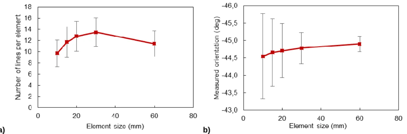
Each 5184 x 3456 pixel image has a resolution of 6.48 pixel/mm with a pixel aspect ratio of 1. An element size of 30 mm per side (in a grid of 20 by 10 elements, thus 200 elements in total) is chosen as good compromise between measurement accuracy and processing time. Figure 4a shows that an element of 30 mm per side contains the largest amount of Hough lines. For all element sizes, the average of the Hough lines orientation is less than 0.4° (cf. Figure 4b). However, the standard deviation of the Hough lines orientations increases drastically when the size of the element is 20 mm per side or lower. The processing time for each ply, with an element size of 30 mm per side is approximately 40 s using a 64 bits Intel® CoreTM i3 processor
a) b)
Figure 4. Hough lines results comparison at different element sizes a) Number of lines and b) mean measured orientation. Error bars indicate ± 1 standard deviation.
Hough lines with angles not within ± 7° tolerance are removed as they are considered as artefacts of the image treatment. The mean angle of the Hough lines is calculated for each element (image segment) to map local orientations. Figure 5 shows orientation maps for 4 different plies in the orientations of 0°, +45°, -45° and 90° respectively. Certain elements in the plies oriented at 0° and 90°are discarded since none of the Hough lines are within the ± 7° tolerance. In average, there are 48 discarded elements for the 0° angle plies and 19 discarded elements for the 90° angle plies. There are not discarded elements for the ± 45° orientation plies.
Figure 5. Orientation maps from plate C-11 showing four different ply directions with a) 0° b) +45° c) -45° and d) 90°.
The main difference of the proposed methodology with the one proposed by Skordos [13], is the method used for capturing the images and the post-processing techniques to obtain the reinforcement orientation. In the proposed method, the complete surface of the prepreg is taken in a single image. The image is corrected for image distortions produced by the optical lens. By having one image, a positioning device for the camera is not necessary. Another difference is in the use of an autocorrelation function coupled with a fast Fourier transform (FFT). FFT algorithms best operate on square images with an area being a power of two, thus limiting the size of the image. The proposed method here uses a Hough transform of a filtered image, the image size is not restricted.
From the orientation maps, variations in the reinforcement orientation across the ply can be noticed with the naked eye. These variations appear to be non-periodic and non-repetitive through the different plies. An identification algorithm is developed to quantify the variation trends in the local fibre orientations.
4. Fibre in-plane misalignments meta-models
It is assumed that the fibres do not move during the curing process. Although, this assumption is not completely true since there is resin flow and evacuation of entrapped air during the first temperature ramp of the curing cycle where the viscosity of the resin is drastically reduced, for practical reasons, it is considered that the shift in the reinforcement position is negligible. Further studies are required to quantify the shift in the fibre position before and after curing.
A number of equations describe the changes in the reinforcement angle for an individual element taking into account a continuity in the values from one element to another (i.e. a maximum value cannot be beside a minimum value).
The reinforcement orientation at any point θk (x,y) of the composite ply can considered as the result of
three different types of orientations (cf. eq. 1): the mean ply orientation 𝜃̅̅̅̅, the periodic fibre misalignments 𝑘
The mean ply orientation 𝜃̅̅̅̅ contains the theoretical ply orientation θ 𝑘 th k (stratification) and an overall
ply misalignment δθk (cf. eq. 2).
𝜃 𝑘
̅̅̅̅=𝜃𝑡ℎ 𝑘+𝛿𝜃𝑘 (2)
The local continuous in-plane undulations θwav are modelled through the form of a sinusoidal wave in
the direction of the ply orientation (cf. eq. 3). The mean amplitude Awav of 0.03 mm and the mean wavelength
λwav of 3 mm, with extreme values between 2.2 and 4 mm, are obtained from the literature [4], [15].
wav k th k k th k wav k th k wavy
x
A
y
x
sin
2
cos
2
sin
2
,
,
(3)It is observed that the in-ply fibre orientations θpert present a non-periodic continuous variations result
from the prepreg manipulation during the lay-up. These local variations of the reinforcement angle can be described by the sum of N pseudo-Gaussian surfaces or perturbations (cf. eq. 4 and Figure 6). This methodology is inspired by Goshtasby and Oneill for 2D curve fittings [19], which was adapted for a 3D surface. 𝜃𝑝𝑒𝑟𝑡(𝑥, 𝑦) = ∑ 𝐵𝑖 𝑁 𝑖=1 𝑒−(( 𝑥−𝑋𝑖 𝛼𝑖 ) 2 +(𝑦−𝑌𝑖 𝛽𝑖 ) 2 ) (4)
where Xi and Yi are the coordinates of the central point of the perturbation in mm, αi and βi are respectively the
length and the width of each ith pseudo-Gaussian surface in mm, and are homologues to the standard deviation in a normal distribution. Finally, Bi is the amplitude of the perturbation in degrees.
Figure 6. Schematic description of the pseudo-Gaussian surface representing the local perturbation in fibre orientations.
5. Results analysis of the optical measurements
5.1. Mean ply misalignment (ply scale)
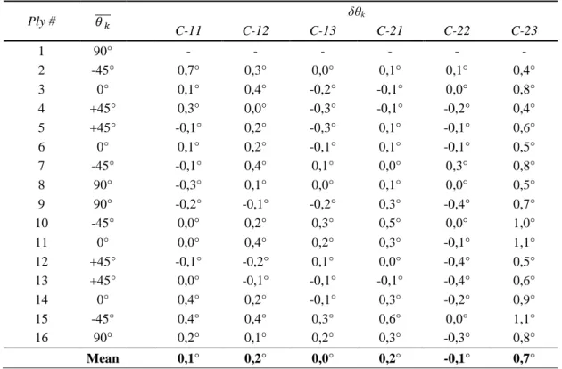
In Table 1 are indicated the values of the difference between the mean ply orientation and its intended orientation δθk, with respect to ply # 1 for all plates. These δθk values were confirmed by manual measuring of
the ply orientation [20]. For plates C-11, C-12, C-13, C-21 and C-22, δθk values range between -0.5° and 0.5°.
For plate C-23, δθk values range from 0.4° to 1.1°. The standard deviation of the ply misalignment for all plates
ranges from 0.30° to 0.40°, the overall misalignment is shifted towards a positive angle. It is assumed that this shift has its origins in the lay-up procedure with the same operators. No correlation was found between the intended ply orientation and its measured misalignment.
Table 1. Difference between the intended ply orientation and measured orientation for all plies and plates referenced to ply # 1. Ply # 𝜃̅̅̅̅ 𝑘 δθk C-11 C-12 C-13 C-21 C-22 C-23 1 90° - - - - 2 -45° 0,7° 0,3° 0,0° 0,1° 0,1° 0,4° 3 0° 0,1° 0,4° -0,2° -0,1° 0,0° 0,8° 4 +45° 0,3° 0,0° -0,3° -0,1° -0,2° 0,4° 5 +45° -0,1° 0,2° -0,3° 0,1° -0,1° 0,6° 6 0° 0,1° 0,2° -0,1° 0,1° -0,1° 0,5° 7 -45° -0,1° 0,4° 0,1° 0,0° 0,3° 0,8° 8 90° -0,3° 0,1° 0,0° 0,1° 0,0° 0,5° 9 90° -0,2° -0,1° -0,2° 0,3° -0,4° 0,7° 10 -45° 0,0° 0,2° 0,3° 0,5° 0,0° 1,0° 11 0° 0,0° 0,4° 0,2° 0,3° -0,1° 1,1° 12 +45° -0,1° -0,2° 0,1° 0,0° -0,4° 0,5° 13 +45° 0,0° -0,1° -0,1° -0,1° -0,4° 0,6° 14 0° 0,4° 0,2° -0,1° 0,3° -0,2° 0,9° 15 -45° 0,4° 0,4° 0,3° 0,6° 0,0° 1,1° 16 90° 0,2° 0,1° 0,2° 0,3° -0,3° 0,8° Mean 0,1° 0,2° 0,0° 0,2° -0,1° 0,7°
The average in the global differences between the intended orientation and the measured fibre directions is inferior to 1.0° with a standard deviation (SD) of 0.35°. The measured values are lower than the values reported by Yurgartis [7] (mean angle of 3.7° and SD of 0.79°) and Olave [21] (mean angle of 1.7° and SD of 0.69°). However, they are in good agreement with the values obtained by Skordos [13] (mean angle of -0.1° and SD of 0.36°). The values of the mean and the SD are characteristic and unique to the studied composite part since they are function of the reinforcement nature and the actual manufacturing techniques used to conform the piece. However, the identification of variation trends are useful to construct and enlarge a database of the different property variations linked to each manufacture steps.
The value of the mean ply misalignment is lower than the initially expected value. In this case, the small deviation is partially due to the size of the ply, where a very noticeable misplacement of 10 mm at one of the corners of the 600 mm long ply is roughly translated into a 1.0° of ply misalignment. Nevertheless, global misalignments can be affected by the shape, size and cutting precision of the prepreg plies. The combination of these factors can conceal significant variations in the ply positioning up to 5° [22].
It has been shown that the measuring method can be used to accurately determine the mean misalignment of the complete ply. A more detailed analysis is required to determine the perturbation misalignments contained within each ply.
5.2. Local misalignments (local scale within a given ply)
The representative values of amplitude, position and shape of the pseudo-Gaussian perturbations that conform the local fibre misalignments, as described in equation 4, are obtained by means of an in-house detection algorithm. The algorithm is set to find values of the 5 variables, Bi, Xi, Yi, αi, and βi, that minimize
the mean square error between the measured misalignments and the generated surface from equation 4.
The algorithm operates in the normalised to zero-mean angle. It is possible that the placement of the centre of any ith perturbation can be outside the edges of the ply, thus this point can be located between -60 and 660 mm in the x-direction and between -60 and 360 mm in the y-direction. Afterwards, the size of the perturbations λi and γi are considered between 30 and 210 mm. Finally, during the analysis of the treated
images, it was found that in any case the maximum difference between any point and the mean ply orientation was within the rage of ± 1°. Thus, it is assumed that the amplitude Bi which the fibres can deviate
between -1° and +1°. It is chosen to use N = 12 pseudo-Gaussian surfaces to form local perturbations in a trade-off between the accuracy, the calculation time and the capability of convergence of the detection algorithm. The computation time for each ply goes from 60 s to 80 s using the same CPU described in section 3.
The shape of the generated surface through the present algorithm using equation 4 is in good agreement with the experimental data by both visual and quantitative analysis. Figure 7 shows the misalignment maps of the reinforcement orientation of a -45° ply for the values as measured by the optical treatment (cf. Figure 7 a) compared to a reconstruction of the same ply (cf. Figure 7b). The measurement error has a mean of 0° with values ranging from -0.2° to 0.2° (cf. Figure 7c). For all treated plies the maximum mean error found is under 0.02° and the maximum standard deviation value is 0.2°. Furthermore, the error scatter in each image is
Figure 7. Misalignment maps comparison for plate C-11, ply #13, oriented at 45° with a) measurement values and b) reconstructed orientations and c) error.
The objective of this methodology is not to introduce the measured misalignments directly into a FE model, but to introduce a computer-generated set of misalignments representative of the observed misalignments. To be representative, the virtual misalignments must have the same order of magnitude and follow the identified variation trends. The image analysis results are used as the basis to obtain the different meta-model coefficients needed to generate the corresponding FE models with continuous variations in the reinforcement angle, using equations 1 through 4.
6. Finite element modelling of the residual strains of a composite plate with varying reinforcement orientation.
In a previous study [2], a FE model was used to determine the variations in residual strains at the end of the cooling phase during manufacturing a composite plate taking into account variations in the ply thickness.
The example here presented serves to determine the influence in the strain field due to local variations in the reinforcement orientation. The analysis is based on the assumption that the composite is stress-free at the end of the curing phase (120°C for the M10.1/CHS composite material). Due to the mismatch of the thermal properties of the constituent materials, a temperature variation induces residual strains and stresses [23].
The FE model uses a shell element type in the LMS Samcef® (Siemens, formerly Samtech, Belgium)
code. The shell composite element allows local control reinforcement orientation for each element and each ply. The complete 600 x 300 mm composite plate is analysed using a 2D Mindlin composite shell (element type T028/T029). The element size is 1 mm per side in order to model reinforcement undulation corresponding to a minimum wavelength of 2 mm. The applied temperature change is ΔT = -100 °C, simulating the cooling step in the polymerisation cycle.
The material properties are presented for a 0.300 mm thick unidirectional ply of M10.1/CHS with a 56 % fibre volume ratio. The typical values for this composite material are shown in Table 2. In this example, only the variation of the reinforcement orientation is taken into account.
Table 2. Mechanical properties of the M10.1/CHS composite ply.
Property Magnitude
Young’s modulus of the composite in the longitudinal direction E1 (GPa)
131.4 Young’s modulus of the composite in the transverse direction
E2(GPa)
9.3 Shear modulus of the composite G12(GPa) 4.3
Poisson’s ratio of the carbon fibre ν12 0.34
Coefficient of linear thermal expansion of the composite in the longitudinal direction α1(°C-1)
- 0.5∙10-6
Coefficient of linear thermal expansion the composite in the transverse direction α2 (°C-1)
14.7∙10-6
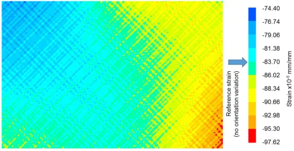
Figure 8 shows the strain field εxx of the upper skin. The deterministic solution strain field εxx, without
taking account any variations, shows a uniform value of -83.4∙10-6 mm/mm (marked as a reference value in
Figure 8), whereas the model accounting for variation in the reinforcement orientation shows compressive strains values ranging from -74.4∙10-6 up to -98.6∙10-6 mm/mm. This represents a variation up to 28 % of the
reference value determined for the deterministic solution, which is significant.
Figure 8. Strain field εxx of the upper skin of a 16-ply 600 x 300 mm composite plate subject to a ΔT = -100°C
7. Conclusions
A methodology to introduce the variation of the reinforcement orientation in FE models of composite structures was presented. This methodology includes the generation of meta-models that describe the orientation variation in the different scales of the composite, for local misalignments and the average ply misalignment. The values that were introduced into the meta-models were obtained from a real composite lay-up by means of automatic image post-treatment.
Image analysis results show that variations in the mean ply orientations are found between -0.5 and 0.5° and the standard deviations range between 0.34° and 0.41°. No correlation was found between the overall ply misalignment and the intended orientation of such ply. The identification algorithm that generates the set of parameters introduced into the meta-models yield extremely good results in terms of calculation time and the misalignments measurements accuracy validated both visually and quantitatively. Finally for the FE model results show variations up to 28 % in the strain field of a composite plate subjected to cooling due only to variations in fibre orientation.
An aspect still unexplored is the interaction between two or more sources of variability. In this paper only the in-plane variation of the reinforcement angle are assessed. Further work is required to introduce the effects of out-of-plane waviness, which can be coupled with a corresponding ply thickness variation. It is important to consider that the sources of variability are highly dependent of the process and material semi-products (i.e. raw materials, composite prepreg, etc.). Hence, great efforts should be conducted to identify and quantify the trends and magnitudes of the different sources of variability that are specific to each application.
Acknowledgements
The authors would like to acknowledge the Consejo Nacional de Ciencia y Tecnologia (CONACyT) of Mexico for providing the funding for the PhD thesis work of Yves Davila.
References
[1] Y. Davila, “Étude multi-échelle du couplage matériaux-procédés pour l’identification et la modélisation des variabilités au sein d’une structure composite,” Université de Toulouse 3 Paul Sabatier, 2015. [2] Y. Davila, L. Crouzeix, B. Douchin, F. Collombet, and Y.-H. Grunevald, “Spatial Evolution of the
Thickness Variations over a CFRP Laminated Structure,” Appl. Compos. Mater., Jan. 2017.
[3] C. C. Chamis, “Probabilistic Composite Design,” Compos. Mater. Test. Des., vol. 13, pp. 23–42, 1997. [4] K. D. Potter, B. Khan, M. R. Wisnom, T. Bell, and J. Stevens, “Variability, fibre waviness and misalignment in the determination of the properties of composite materials and structures,” Compos. Part A Appl. Sci. Manuf., vol. 39, no. 9, pp. 1343–1354, Sep. 2008.
[5] R. S. Trask, S. R. Hallett, F. M. M. Helenon, and M. R. Wisnom, “Influence of process induced defects on the failure of composite T-joint specimens,” Compos. Part A Appl. Sci. Manuf., vol. 43, no. 4, pp. 748–757, Apr. 2012.
[6] Y. Arao, J. Koyanagi, S. Utsunomiya, and H. Kawada, “Effect of ply angle misalignment on out-of-plane deformation of symmetrical cross-ply CFRP laminates: Accuracy of the ply angle alignment,” Compos. Struct., vol. 93, no. 4, pp. 1225–1230, Mar. 2011.
[7] S. W. Yurgartis, “Measurement of small angle fiber misalignments in continuous fiber composites,” Compos. Sci. Technol., vol. 30, no. 4, pp. 279–293, Jan. 1987.
[8] S. Barwick and T. Papathanasiou, “Identification of fiber misalignment in continuous fiber composites,” Polym. Compos., no. 3, pp. 475–486, 2003.
[9] C. J. Creighton, M. P. F. Sutcliffe, and T. . Clyne, “A multiple field image analysis procedure for characterisation of fibre alignment in composites,” Compos. Part A Appl. Sci. Manuf., vol. 32, no. 2, pp. 221–229, Feb. 2001.
[10] K. Kratmann, M. P. F. Sutcliffe, L. Lilleheden, R. Pyrz, and O. Thomsen, “A novel image analysis procedure for measuring fibre misalignment in unidirectional fibre composites,” Compos. Sci. Technol., vol. 69, no. 2, pp. 228–238, Feb. 2009.
[11] M. P. F. Sutcliffe, S. L. Lemanski, and A. E. Scott, “Measurement of fibre waviness in industrial composite components,” Compos. Sci. Technol., vol. 72, no. 16, pp. 2016–2023, Nov. 2012.
[12] G. Requena, G. Fiedler, B. Seiser, P. Degischer, M. Di Michiel, and T. Buslaps, “3D-Quantification of the distribution of continuous fibres in unidirectionally reinforced composites,” Compos. Part A Appl. Sci. Manuf., vol. 40, no. 2, pp. 152–163, Feb. 2009.
[13] A. A. Skordos and M. P. F. Sutcliffe, “Stochastic simulation of woven composites forming,” Compos. Sci. Technol., vol. 68, no. 1, pp. 283–296, Jan. 2008.
[14] T. S. Mesogitis, A. A. Skordos, and A. C. Long, “Non-crip fabrics geometrical variability and its influence on composite cure,” in ECCM 16, 2014.
[15] K. D. Potter, C. Langer, B. Hodgkiss, and S. Lamb, “Sources of variability in uncured aerospace grade unidirectional carbon fibre epoxy preimpregnate,” Compos. Part A Appl. Sci. Manuf., vol. 38, no. 3, pp. 905–916, Mar. 2007.
[16] L. Shi and S. Wu, “Automatic Fiber Orientation Detection for Sewed Carbon Fibers,” Tsinghua Sci. Technol., vol. 12, no. 4, pp. 447–452, 2007.
[17] C. Redon, L. Chermant, J. Chermant, and M. Coster, “Automatic image analysis and morphology of fibre reinforced concrete,” Cem. Concret Compos., vol. 21, pp. 403–412, 1999.
[18] J. Canny, “A computational approach to edge detection.,” IEEE Trans. Pattern Anal. Mach. Intell., vol. 8, no. 6, pp. 679–98, Jun. 1986.
[19] A. Goshtasby and W. D. Oneill, “Curve Fitting by a Sum of Gaussians,” CVGIP Graph. Model. Image Process., vol. 56, no. 4, pp. 281–288, Jul. 1994.
[20] Y. Davila, L. Crouzeix, B. Douchin, F. Collombet, and Y.-H. Grunevald, “Quantification of sources of variability in CFRP plates cured in autoclave,” in International Conference on Composite Materials 19, 2013.
[21] M. Olave, A. Vanaerschot, S. V Lomov, and D. Vandepitte, “Internal Geometry Variability of Two Woven Composites and Related Variability of the Stiffness,” Polym. Compos., pp. 1335–1350, 2012. [22] M. Torres, B. Douchin, F. Collombet, L. Crouzeix, Y. Grunevald, and R. Bazer-bachi, “Valeur ajoutée
d ’une encapsulation de capteurs silicium pour l’instrumentation à cœur des structures composites,” in JNC 17, 2011, pp. 1–10.
[23] M. Mulle, F. Collombet, P. Olivier, R. Zitoune, C. Huchette, F. Laurin, and Y. Grunevald, “Assessment of cure-residual strains through the thickness of carbon–epoxy laminates using FBGs Part II: Technological specimen,” Compos. Part A Appl. Sci. Manuf., vol. 40, no. 10, pp. 1534–1544, Oct. 2009.