Labor and investment demand at the firm level: A comparison of French, German and U.S. manufacturing, 1970–79

LABOR AND INVESTMENT DEMAND AT THE

FIRM LEVEL: A COMPARISON OF FRENCH,

UERMAN AND U.S. MANUAU1U1UNU, i9(U—(#

Jacques Mairesse Brigitte Dorinont

Working Paper No. 15514

NATIONAL BUREAU OF ECONOMIC RESEARCH

1050 Massachusetts Avenue

Cambridge, MA 02138

February 1985

The research reported here is part of the NBER's research program

in Productivity and project in Productivity and

Industrial

Change

in the World Economy. Any opinions expressed are those of the

NBER Working Paper #1554

February 1985

Labor

and Investment Demand at the

Firm Level: A Comparison of French,

German and U.S. Manufacturing, 1910—19

ABSTRACT

We investigate how labor and investment demand at the firm level

(gross as well as net and replacement investment separately) differs in French, German and U.S. manufacturing, and has changed since the 1974—75

crisis. We use three consistent panel data samples of large firms for

1970—79, and rely on simple models of the accelerator.-profits type. We find

that the accelerator effects and the profits effects did not vary much

between 1970—73 and 1976—79, and were quite comparable in the three countries, the former being of a more permanent nature and the latter more transitory.

To a large extent these effects account for the important changes and differences in labor and investment demand between the two subperiods and

across the three countries.

Jacques Mairesse Brigitte Dormont

Institut National de la Statistique Universite de Paris

et des Etudes Economiques IX — _Dauphine

18, Boulevard Adoiphe—Pinard 75016 Paris

75675 Paris Cedex 114 France

I — INTRODUCTION

The first oil shock at the end of 1913 marked a considerable break in the

economic evolution of France, Germany, the tJnited States and other industrial

countries. For the first time in thirty years ("Les trente glorieuses"),

aggregate industrial production dropped: this happened in 19114 in Germany and

the United States, in 1915 in France. Since then the economic situation has not recovered to what it was before; most industrial countries have experienced weaker growth, with a slowdown in capital accumulation and rising unemployment. Many macroeconomic studies, a number of them in a comparative perspective, have tried to analyse and understand the various issues at stake. The present work is part of an effort to complement and enrich these studies, by considering some of the same issues at the microeconomic level, i.e., using firm panel data

instead of aggregate time series.1

Our purpose here is to investigate whether the behavior of firms in

regard to labor demand and investment demand (gross investment as well as net investment and replacement investment separately) is similar in the French, German and U.S. manufacturing industries, if not how it differs, and whether it has been stable before and after the 197141975 crisis, if not how it changed.

To accomplish this we had to construct consistent and comparable data sets for French, German and U.S. manufacturing firms over a long enough period

(1966—1919). In view of the formidable complexities of the formal modelling of

factor demand decisions, as well as the lack of good information on

—2--as regards expected factor prices at the firm level), we resorted to simple

models of the basic accelerator profits type. Further, of the many

possibilities in structuring the data and specifying the estimated equations,

we have chosen two: year to year growth rates and average growth rates. We have also kept the seemingly necessary minimum number of lags in the regressions. We

thus bypass some of the difficulties of the econometrics of panel data.

It is necessary to define the scope and meaning of our study by giving

some explanations of these matters, i.e., sample construction and the

measurement of variables, choice of model and interpretation, specification and estimation considerations. We shall do so in the first part of the paper. We

shall then present the empirical results and comment on them in the second part. We concentrate on the estimates of the accelerator profits equations, but we shall also report on some attempts to use additional explanatory variables on

II

- _{GENERAL FRAMEWORK AND BACKGROUND} CONSIDERATIONS 2.1. On Samples and Variables

We have constructed our samples of firms for all three countries along the same lines. However, due to the different characteristics of the data banks

from which we drew these samples (range of firms, extent of missing observations

or large errors, proportions of firms entering, leaving or going through a major

merger), we cannot consider them as truly representative in any definite sense.2 They consist of 307 French firms, 1145 German firms and 422 U.S. firms, for which we have complete data for our main variables over the l4 years 1966—79.

Although these firms are only a small cohort out of the total number of

manufacturing firms, they are relatively large companies, and they account for

about I

and

8

_per

_{cent, 9}

to

10 per cent and as much as 50 per cent of total

employment in French, German and U.S. manufacturing industries respectively. Their average sizes reflect the well known fact that U.S. firms are generally

much larger than their French and also German counterparts: the geometric means

of the number of employees being about 1000 in the U.S. sample as against 700

and 11400 in the French and German samples, respectively. Because our

regressions

involve three lags, our study period is in fact restricted to the 10

years 1970—79, i.e., four years before and four years after the l9714_75

break.

We have defined and measured our basic variables as similarly as possible

for the three samples. With the major exception of the physical capital stock variable in the case of the German sample, they can be considered as closely comparable. Labor L is measured by the total number of employees (average number

over the year). Both for France and the U.S., gross capital stock C is taken as the gross book value of fixed assets following an adjustment for inflation

which involves a rough estimate of average age.3 For Germany, such a measure is

not possible and we constructed C as the sum of past investment expenditures

based on a fixed average service life of i6 years. This required a

retrapolation of the investment series for our firms before 1961 on the basis of

the corresponding industry growth

rates)

Gross investment I is measured as the

total capital expenditures in plant and equipment deflated by the industry investment price indices. However, these investment numbers happened to be

generally missing in the accounts of our German firms before 19714, and we had to

compute them as the yearly change in the net book value of fixed assets plus the depreciation charges in the same year. Thereby we neglect corrections for

acquisitions, disacquisitions or revaluations of assets. But though our

investment variables are not strictly comparable for Germany, the problem in this case would seem to be less severe than as regards the capital stock

measure. Output Q is defined as sales deflated by the available industry output price indices.5 Profits P are taken as gross operating income adjusted for

inventory changes, i.e., production less total cost of goods sold or value added

less labor cost.6

In order to assess the possible influence of the inconsistency between

our capital and investment measures for our three samples we also estimated the investment series for France and the U.S. in the same way as for Germany, and

the

capital stock figures for all three using the permanent inventory method

obtain

with these alternative measures are not on the whole too different from the ones we find with our main measures, and they lead essentially to the same

conclusions. This is apparent in the estimates we present in the Appendix I.

The actual variables that we use are the rates of growth of labor, capital and output: DL, DC and DQ (computed as the first differences in Log L,

Log C and Log Q, respectively), the ratio of gross investment to the capital I/C and the profit rate PR (computed as P/CV where CV is the value of the capital in

current prices, i.e., the value in constant prices C multiplied by the

appropriate investment prices indices). The two variables I/C and DC can also

be termed the gross investment rate and the net investment rate, respectively, and their difference (I/c — DC) measures the proportion of capital that has been

retired or scrapped, that is the ratio of replacement (and modernization) investment to capital, or the replacement rate B/C for short.8 This variable

is of course bound to suffer from all measurement errors affecting both our

gross and net investment rates I/C and DC, and from the discrepancies between the two. We can expect however, that in the case of the French and the U.S.

samples it conveys some useful and genuine information about the true

replacement investment. Since so little is known about replacement ("The other half of gross investment" Feldstein and Foot, 1911), it seemed interesting to consider it explicitly in our investigations of these two samples. In the case

of the German sample, by virtue of our

construction

of the capital stock measure, the replacement rate can only reflect (after some smoothing) the proportion of investment expenditures 16 years ago to the capital stock at

present. However, we also consider this rate in that case so as to get a better

—6—

2.2.

On Resorting to the Accelerator Profits Model

As M. Feldstein (1982) put it in a somewhat provocative way "the

investment process is far too complex for any single model to be convincing,...

and the applied econometrician, like the theorist, soon discovers from

experience that a useful model is not one that is "true" or "realistic" but one

that is parsimonious, plausible and informative". We shall take up such a stand

in this study —

which

is not so humble an attitude as Feldstein seems to suggest but already a quite ambitious claim.

At

least four factors should a priori enter, and be tested as important

determinants,

in a behavioral model of

the investment demand and (or) the labor

demand

by firms: expected output demand, expected profitability, the relative expected cost of labor and capital, and, to the extent that capital markets are imperfect, the actual current and past profits (or the financial liquidity of the

firm). Except for the last one, these factors are generally unobservable. Moreover the way they should intervene in the model equations should

specifically depend on the form of the production function (for example whether it is Cobb—Douglas or CES, or more importantly "putty—putty" or 'putty—clay"), the form of the costs of adjustment functions (or that of other relevant

constraints), and the nature of the firms' objectives, expectations and market environment.

Being aware of such basic complexities and being bounded by the limitations of our data, as well as relying on the empirical findings of

numerous econometric studies of factor demand, we had recourse to an accelerator

formulation,

i.e., investment and labor change equations rather than capital

stock and labor ones. This formulation can be advocated on various grounds. Tt provides equations which are conveniently linear both in the current and past changes of sales and in the current and past levels of profits. It can be viewed as a way to deal simply with the heteroscedasticity associated with the large differences in size of firms. It is also related to other more profound

econometric issues of specification and estimation, as we shall show below. The relations that we choose to estimate are thus of the following form:

£

1 2

DL or DC or I/C or R/C =

c0 + a

DQ +

b.PR

j=O j=O

In fact we used industry dummies (16 of them for each country) instead of a

simple constant c0.9 Experiments with various lags have also shown that besides

the current values three lags for sales growth rates (2. = 3) and one for profit

rates (L2 = 1) were sufficient and did not oblige us to shorten our study

period too much. This is documented in the Appendix II, in which we provide the

estimates of the total accelerator effects when using no lags, three and five

lags and geometrically decreasing lags in the autoregressive form. For reasons to be given below we have at the same time estimated "long run versions" of our

regressions with no lag and using average growth rates instead of the year to year ones:

or or Tf7

or

= c +

(a

)•

+ (Eb

)

The precise motivation and interpretation of the accelerator profits

—8—

account

can he found in R. Eisner's 1978 book, which recapitulates his

investigations pursued during nny years on the individual firm data of

McGraw—Hill capital expenditure surveysJ0 Although it properly concerns gross

investment or net investment, to a large extent the same line of arguments

applies to labor demand. We would expect, however, the profits effects to be

smaller for labor than for investment, and the accelerator effects more rapid. The accelerator profits model can also be extended to the replacement investment demand, but in this case one would expect much smaller accelerator effects or even "decelerator effects".

Investment and labor hiring decisions are essentially forward—looking and

depend on expectations. The more irreversible these decisions are (i.e., the

more "fixed" capital and labor factors or the higher their costs of adjustment),

the longer the time horizon of the relevant expectations. Thus only the sales

increases which firms perceive as long term or permanent will lead to net

investment and hiring, while short term or transitory changes will he generally

met by changing the hours of work and the utilization of existing capital. In that respect perhaps the most drastic simplification of the accelerator model

(and of most other factor demand models as well) is the substitution of current

or past variables for anticipated future ones. It reflects the underlying

investment and labor demand behaviors to the extent that firms view their

current and past changes in sales as permanent. The proper meaning of the model

is thus related to the validity and stability of the relationship between changes, or revisions, in expected output demand and observed current and past changes in sales, as much as it is to that of other behavioral assumptions and

the form of the production function. The accelerator model is just a convenient short cut through an intricate system of relations and conditions. It should be gauged by its empirical significance and robustness and not by its appeal or status. When looking at our estimates for the different country samples and

subperiods, we shall be at best comparing an overall average outcome of the processes by which firms have been forming their anticipations and on that basis have reached their investment and employment decisions.

Within such a general interpretation of the accelerator model, the

appreciation of the respective roles of sales changes and profits warrants some

discussion. It might seem intuitively appealing to take the sales change

variables as a proxy for changes in expected demand, and the profit variables as a proxy for expected profitability as well as an indicator of the financial

liquidity of the firm. The finding that only current and one—year lagged past profits come out to be statistically significant (as well as the fact that their

estimated coefficients are larger in the regressions on the year to year growth rates than in the ones on the average growth rates) mainly supports the

financial liquidity interpretation. On the other hand, it is plausible that profits would also convey information about the future demand addressed to the firm, and past sales changes information about its future profitability. To

make the interpretation more clear—cut (though controversial), we can break this a priori symmetry by taking the view that all the relevant information about future demand (at least that which is more specific to the firm) pertains to the sales changes variables only, although all this information is not directly

—10—

Eisner's example, we will be justified in computing full or total accelerator effects as the sum of the direct effects of sales changes and of the indirect

effects through profits. These total effects are the ones we would obtain if we had a pure accelerator model, and this is a simple way in practice to compute

them (i.e., by omitting the profits variables and keeping only the sales changes variables in the estimated regressions).

2.3. On Year to Year and Average Growth Rates Estimates

Panel samples such as ours offer a number of possibilities for

structuring and handling the data, which lead to various types of estimators. In the case of a standard linear regression model, if it is well specified,

these various estimators should all be consistent. Conversely, their

differences when significant imply some sort of specification errors, and this can provide formal specification tests (see for example Hausman and Taylor,

1981). More interestingly, if one is ready to be specific about the kind of

misspecification occurring, these differences can be used to retrieve the

characteristics and orders of magnitude involved in such misspecification. For

instance, it is possible to assess the importance of correlated specific effects (possibly due to the omission of unobserved firm characteristics in the model) or that of random errors in variables, which are the two specification errors

usually

put forward. Comparing estimates for different structuririgs of data can

contribute to a richer understanding and knowledge of the model and the data, as

well

as to a better awareness of their limits.

The most usual transformations applied to panel data (and the

whether or not they remove the individual specific effect u. in an error components model (where the overall error term e. is decomposed into two

independent terms u. + the subscripts i and t standing for firm and year,

respectively). In general, when the original variables are in levels (or in

logs of levels or in the form of more or less structural or stable ratios), the

variability of the individual effect u is largely predominant, and the two

groups of transformations can be viewed as providing cross—sectional and time

series type estimates, respectively. The total estimates performed on the

untransformed variables y and the hetr-ri—trm estimates performed on the

it

firm means y. belong typically to the first category. The within—firm estimates

relying on the deviations to ;he trm means

), the

first difference or

long—difference estimates using the year to year differences

or

their average over a given period are the usual candidates

in the second category. When starting with a model in logarithms, which is our

case, first and long differences correspond to yearly and average growth rates, respectively.

The general view is to believe that the individual effect u1 is more

likely to be seriously correlated with the explanatory variables than the disturbance w.t, and therefore that time—series type estimates would be the

better, less biased ones. Although this view may

be

controversial (see

Mairesse, 1918 and Griliches and Mairesse, l984), we shall go along with it here.11 However, one of the important drawbacks of the time series estimates is that they tend to be quite sensitive to random errors of measurement in the variables. This is specially true of the first—difference estimates, but less

—12—

so

for the long—difference estimates, inasmuch as they will average out over a

long period such errors. Long—difference estimates (and to a lesser degree within estimates) have thus the specific advantage of reducing the errors in

variables

biases (see Griliches and Hausman, 19814).

Unfortunately, on the other

hand,

taking long

differences does not permit in practice to estimate the lag structure

of the explanatory variables in a dynamic model

such as the

accelerator—profits

model. Unlike first differences (which are often quite

moderately

correlated) the long differences of lagged variables are bound to be

strongly collinear. Hence, the

estimates of the individual lagged coefficients

are

bound to be very imprecise and unstable,; furthermore, even relatively minor errors of measurement in the variables would result in aggravating this problem. In fact, we can only expect to estimate well the sum of the coefficients.

Since the current values act as excellent proxies of the lagged values, there is

not much sense in specifying lags in a model to be estimated on long

differences. In the version without lags the estimated coefficient will be the

long—run coefficient, corresponding to the sum of the lagged—variables

coefficients in the model with lags. Similar considerations largely apply to

the within estimates, which are not better than the long differences estimates

in that respect; moreover, in short panels they will also suffer from

serial-correlation biases.

In our context, the first and long difference estimates (i.e., the estimates on yearly and average growth rates) can be given a more specific

interpretation, and this is a further reason to consider both types. By

transitory sales changes or profits, and the fact that firms in their labor and

investment decisions will typically respond much more strongly to permanent sales changes than to transitory changes, and that conversely they will react

more markedly to transitory than to permanent profits. If we are willing to

accept some extreme simplifications, we can give a more definite meaning to

these notions and infer what are the orders of magnitudes involved. Trying to make less stringent assumptions would lead us in fact to adopt a vector

autoregressive framework in the line of Mairesse and Siu (vAn extended

accelerator model of R&D and physical investment", 19R)4). We present a more

—l4—

III.

PRESENTATION AND ANALYSIS OF THE RESULTS

3.1. Looking at the Average Record

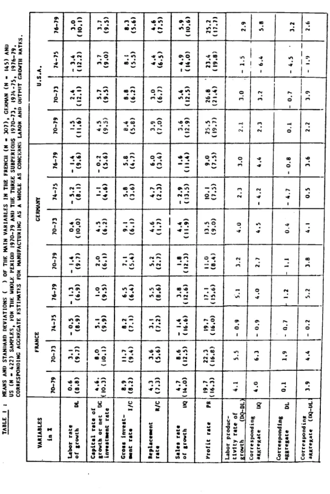
Table 1 lists the means (in %) and standard deviations of our

main variables: the labor, capital and sales rates of growth (DL, DC, DQ) and

the gross investment, replacement and profit rates (I/c, R/C, PR). These are

given for the three samples, the overall period 1910—79, and the three

subperiods: 1970—73. 197)4—75 and 1976—79. We also give corresponding "macro"

figures for the growth rates of total employment and output (i.e., the aggregate

estimates for manufacturing in the three countries). For the convenience of

comparison, we have added the growth rates of labor productivity (DQ — DL)

implicit in these numbers for our samples and manufacturing as a whole. When looking at such averages computed from "micro" data, and in

particular

if

one brings them together with similar "macro"

figures,

one should

be

_quite

aware of the many discrepancies that could arise from the selection of

the

samples and the measurement of the variables. Among other things, computing

unweighted

rather than weighted averages, or using even close variants to adjust

variables —

for

example deflating them with different prices indices which may

be available for more or less disaggregated industrial breakdowns —can really

matter. It is our experience, however, that even in these cases when the

discrepancies on averages could be large, the second order characteristics (standard deviations and correlations), especially if they concern relative

magnitudes (or logs), will not be significantly affected in general. Thus the

as the ones we will be considering next -

are

usually quite robust.'2

Another difficulty —

but

a usual one this time — when _{comparing averages}

of growth rates is that they may be very sensitive to the exact periods on which

they are computed (and particularly if it is not possible to choose beginning year and end year occupying similar positions in the business cycle). Despite

these warnings of caution about averages, the general picture they provide in

Table 1 seems quite consistent, and would deserve a number of comments. We

shall limit them to a few observations, leaving to the interested reader to look into more details.

For

our three samples as well as for manufacturing as a whole in the

three countries, the two years 191)4—1915 mark a severe break. Employment and

output

dropped in absolute terms by as much as 10% for employment in Germany,

and 10% for output in the U.S. It is noteworthy that by dismissing workers to

such an extent Germany was able to maintain gains in labor productivity even in these two years, unlike France and the U.S.

Although the 197)4—75 crisis seems to have hit the three economies with similar force, their relative situations before and after have changed a great

deal. Between 1910—73 and 1976—79, in both the French and German samples,

output growth has been slowing down strongly, net and gross investment have

dropped drastically and employment has started diminishing. The firms in the U.S. sample on the contrary appear to have recovered completely: their

production and labor force have been growing even more rapidly. These trends are confirmed by the aggregate numbers on output and employment for

—i6—

deceleration

observed for France and Germany is much more marked in our samples than in the aggregate, while conversely for the U.S. the acceleration is more

pronounced in the aggregate than in the sample. Such a discrepancy which is

strikingly similar for our three samples might be explained by a comparable selection bias: by selecting firms which are in existence over a long period, we necessarily exclude the new—corners which are plausibly more rapidly growing

firms; we also exclude firms growing through major mergers.

It is also interesting to underline the comparable increase in the replacement investment ratio between the two periods for our three samples. As it is clear from the computation of this ratio in the German case, this

increase reflects the slowdown in the stock of capital; in the cases of France and the U.S. it may also illustrate to a certain extent what is often said about the shortening of capital service lives and the acceleration of obsolescence.

Last, the differences in the average levels of the rate of profits computed for

our three samples should be taken as very dubious, and particularly the much

lower rate in Germany. Such shortcoming does not preclude of course that these measures should be good proxies for the true differences (between firms) and

changes (within firms) in the rates of profits for each sample separately.

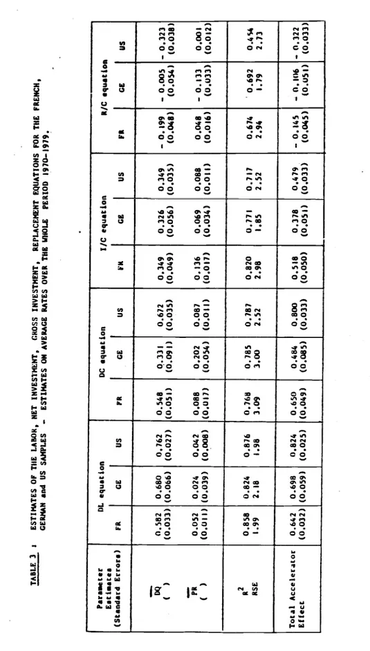
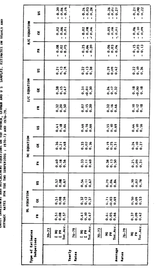
3.2. Comparing the Accelerator and Profit Effects Between Countries and Periods

Comparing our estimates (sales changes and profits coefficients) for the

four equations of interest (labor and capital growth rates, gross investment and replacement rates), the two types of estimates (on yearly and average rates),

leave aside 1975—76), involves indeed a lot of numbers. We shall try to go through them in just about that order, looking at the differences first between the two types of estimates, then between countries, last between periods. The

estimates of the two types are respectively given in Table 2 and 3 for the four

equations by three countries. Since, by and large, as we shall see, these esti-mates do not change much from the first to the second period, they are only

given in full detail for the overall period 1970—79. The sums of sales changes

coefficients (or direct accelerator effects) and of the profits coefficients (or profits effects) have been also computed in Table 2; they are directly

com-parable to the (unique) sales changes and profits coefficients in Table 3. In

addition, the total accelerator effects (obtained from running the same

regressions without the profits variables) are presented in the last lines of Table 2 and 3. Both types of estimates of the direct and total accelerator

effects and profits effects are recorded in Table 4

for

the two periods 1970—73 and 1976—79 separately. Last, Table 5 highlights the contributions of our models in explaining what are on average our labor and investment variables

during the two periods, and in explaining their average changes between these two periods.

Permanent

Versus Transitory Effects

Our first general observation on Tables 2

and 3 is that

the pattern of

differences

between our two types of estimates of the accelerator and profits

effects is always the same for the different equations across countries. With only very few exceptions, the estimates of the accelerator effects on average

—18-.

rates (i.e., long differences in logs over 10 years) are larger by about 20 to

50% than the estimates on yearly rates (i.e., first differences in logs). The

reverse situation is true for the profits effects: the average rates estimates

are

smaller in about the same proportions than the yearly rates estimates. The

same pattern of differences is also visible, but much less consistently so, in

Table

)4, when we consider the corresponding estimates for the two periods (long

differences in logs over 14 years only and first differences in logs).

Such a pervasive finding extends the similar results obtained by Eisner (1918) and Oudiz (1978) for the gross investment equation on their respective

samples of U.S. and French firms. It illustrates clearly the importance of the distinction between permanent and transitory effects. Firms tend to view their

actual sales changes as partly transitory and are cautious not to alter their

labor and investment demands in response to these transitory fluctuations. They take their labor hiring and investment decisions on the basis of expectations of

their future output demand, and they form these expectations on the basis of their past sales changes to the extent that they consider these changes

permanent. Granted the assumptions and simplifications indicated in the

Appendix III, it is possible to give more substance to such interpretation and

to retrieve tentative orders of magnitude by comparing the two types of estimates. The weight of the transitory component (relative to that of the

permanent component) in the total variance of sales changes practically vanishes

when going form yearly rates to 10 years average rates (from roughly about 25% in the three countries down to less than 5%). The finding of smaller estimates

to what extent the elasticity of firms own demand expectations is smaller in

response to transitory sales changes than in response to permanent ones. The "transitory

elasticity" could range from 0

to 0.20 and the "permanent

elasticity"

from 0.60 to 0.80 on

the basis of the orders of magnitudes found for

the labor and investment equations in the three countries (i.e., total

accelerator effects in the range of 0.5 to 0.6 and of 0.6 to 0.8 when estimated

on yearly rates and 10 years average rates, respectively).

Beyond the numbers themselves, these results point to the fact that the accelerator effects should not be simply conceived as technological parameters

(to be equal to 1 in the long run assuming constant returns to scale and neutral

technological progress in production for cost minimizing firms). It makes a more plausible story to consider them as also dependent on the elasticities of

firms sales expectations (or even to strictly identify them with such elasticities).

Turning to the profits effects, the interpretation runs in the same way but with reverse implications. The transitory profits effects are higher than the permanent ones. Firms tend to hire more labor and to invest more in the years when they make higher profits or in the years that immediately follow them, even if they perceived these profits as short run. They do not, however,

sustain such decisions to a comparable extent, whenever the higher profits

persist. In other words there is a timing influence of profits. Firms which may encounter difficulties in borrowing on financial markets will accelerate or

delay their investments as well as their labor hiring decisions depending on

good or bad profits. Looking at the tentative orders of magnitude under the assumptions of Appendix III, the weight of the transitory component in the total

—20—

variance of profits could be as high as 50 percent in terms of the yearly rates,

and be reduced to about 10 percent in terms of the 10 years average rates. On this basis the transitory and permanent profits effects would be respectively of about 0.15 and 0.05 for labor demand and 0.20 and 0.10 for net investment demand

(taking 0.10 and 0.05 as the estimates of the profits effects on yearly rates and 10 years average rates respectively in the labour equation and 0.15 and 0.10 as the corresponding estimates in the net investment equation).

Differences Between Countries

Our second general observation on Tables 2 and 3 is that the differences

between countries for the four estimated equations are for most of them

relatively small; although they may be statistically quite significant, they

usually correspond to orders of magnitude which are roughly the same. The

prevailing impression is one of overall similarity, showing that in fact the labor and investment demand behaviors of the large manufacturing firms making up our samples are largely comparable in France, Germany and the U.S.

Concentrating on the total accelerator effects, and considering chiefly

the average rates estimates (i.e., practically the permanent effects) to make

comparison easier, these effects are of about 0.6 to 0.T for both labor and net

investment demands in France and Germany. The smaller coefficient in the net

investment equation for Germany is in fact not statistically different from the French one; to some extent it may also reflect the difference in the measurement of the capital stock variable for Germany (as we can gather from the estimates using more comparable measures in Annex I). The accelerator effects appear also

to be almost equal for the two equations in the U.S., but of somewhat higher

order of magnitude (0.8).

Looking at the gross investment equation instead of the net investment

one, the total accelerator effects are well reduced, being about O.)4 to 0.5 in the three countries. These reductions correspond to the "decelerator effects" apparent in the replacement investment equation. Such effects are particularly

important for the U.S. sample, less so but still manifest for the French sample, and not really significant for the German one.

As we explained, in the case of Germany, the replacement rate is by

construction the proportion of 16 years ago past investment to current capital

stock. Thus we expected to find zero effects for the German replacement

equation. If we consider them altogether, the estimates we get are indeed quite poor. The sales changes coefficients are clearly insignificant. The profits

coefficients, though, come out significantly negative for our two types of

esti-mates. Such result may seem strange and could be spurious. They may also

simply reflect the fact that firms with a relatively low R/C ratio (the way it is calculated in the German sample) are rapidly growing firms with relatively

high profits. In the case of France and the U.S., the evidence for decelerator effects appears strongly by way of contrast with Germany. The total decelerator effects would be of about —0.30 in the U.S. and of about —0.15 in France. If we

look, however, at the estimates by subperiods in Table 4,

there

is clearly a change occurring for France: the decelerator effect, which was smallish before 1974—75, becomes quite important after and comparable to what it is for the U.S.

—22—

replacement investment ratios for French and U.S. firms, it would seem that we

can attach credence to the finding of sizeable decelerator effects in these two cases. Other things equal, firms tend to increase their replacement and

moder-nization investments when their sales slow down and their expected capacity

needs get weaker; conversely they tend to diminish them when they anticipate that their capacity needs will intensify. In France such behavior seems to have really come into action only since the l9T4—T5 crisis. This might confirm —

in

a perhaps less ambiguous way than the increase of the average replacement rate

—

_the

widespread beliefs about the acceleration of obsolescence.

Turning to the profits effects, they appear more variable between the

different equations and also across countries than the accelerator effects. If we put aside the replacement equations in which the influence of profits seems

rather dubious (for Germany as we have said, but also for France and the U.S. where this influence is at best small and tends to go in opposite directions),

the profits effects are clearly smaller in the three countries for labor than

they are for net and gross investments. This may be considered as another

indi-cation of the predominance of the financial role of the profits variable in our

equations. One noticeable difference between the three countries is that one year lagged profits have the largest impact in France and Germany relatively to

current profits, while the opposite is true for the U.S. Apparently American

firms react almost immediately to the good or bad news about their profits, and French and German firms are slower in their responses.

Some last remarks are worth mentioning about the time profile of the accelerator effects and the relative importance of the direct and total acce—

lerator effects. If we compute the proportion of the accelerator effects taking

place in the first year, it is of about 60 percent for labor in both France

and Germany, and as much as 80 percent in the U.S. It is much less but still high, about a third, for gross and net investment in the three countries. The

proportion of the direct accelerator effects (working through sales changes

only) to the total effects (transmitted also via profits) is overwhelming and pretty much the same in the three countries: on the order of 90 percent for

labor, and 60 to 80 percent for net and gross investment.

Changes After l9T4—T5

Examining thoroughly in Table I the various estimates of the accelerator

and profits effects obtained for our two periods 1910—T3 and l9T6—19, the

general conclusion is one of no drastic changes and of a relative overall

stabi-lity. Although economic environment altered vastly and mostly for the worse,

firms have sustained basically the same labor demand and investment demand beha-viors, as characterized in our equations and variables.

However, a general tendency towards both smaller accelerator effects and

smaller profits effects is clear, these coefficients being reduced on average by

as much as one fourth in the second period relative to the first one. An excep-tion, that we have already stressed, is the appearance of a sizeable decelerator

effect for replacement investment in France after l91I_T5, which is comparable

to the one found for the U.S. Of course, such a reduction in our estimates does not necessarily mean that the "true" accelerator and profits effects, in as much as they have a structural interpretation, are really undermined; it could mdi—

— 21—

cate

that a factor of importance omitted in our equations (and correlated with

sales

changes and profits) has come specifically into play. One might see there

the influence of the overall economic climate and of the future prospects of the

various industries, which contribute to weaken or reinforce firms expectations in their own sales and profits.

A better insight into the characteristics of our models and their com-parative performance in the two periods is provided by the detailed information

recorded in Table 5. We have computed in this table the results of applying

directly our estimated equations to the average situations in the two periods (two first columns for each country), as well as to the changes between the two

of them (third column obtained by difference). Besides the R2 and the standard

errors on the estimated coefficients, this is another way of assessing the explanatory value of a model and the respective contributions of its variables. For these computations, we used the estimates derived from the 10 years average rates (given in Table 3) and the means of the variables for the two periods

1970—73 and 1976—79 (given in Table i). We thus obtain the direct and indirect

accelerator effects (DA and IA lines respectively in the Table 5), and the own

profits effects(OP). In order to fully account for our variables of interest,

(i.e., average labor and capital growth rates DL and DC, average gross investment

and replacement rates I/C and ) we are left with residual constants, summing

up the independent contributions of all other ignored factors. In an attempt to

go one step further, we distinguish in these residuals the part which would correspond to shifting coefficients in our equations, ie.., the variation in the value of the residuals, using the different estimates found for the two

periods separately instead of the ones obtained for the overall period. This

part we note DCst in Table 5, and the remaining one Cst.

After these necessary explanations on the contents of Table 5, our com-ments can be straightforward. We shall leave aside the replacement equation, in which the decelerator and profits effects tend to be at best small and offset

each other (and thus the "constant" remains most of the story). For the labor,

net and gross investment equations, the results are fortunately much more

satis-factory. The direct accelerator effects (DA) very often play the largest role,

for example in explaining the severe fall in average labor growth or in net and gross investment rates after l97)-—75 in France and Germany. The profits effects are in general quite sizeable, even considering only the own effects (OF) and taking apart as we do the indirect accelerator effects (IA), which usually

constitute a fair share of the total. As could be expected, the shifting

coef-ficients effects also contribute appreciably to explaining the changes which

occurred between the two periods. Finally, in many instances, the constants or residual factors effects (Cst) do not appear as predominant; if they tend to

account largely for the average situations in the two periods, they have often

enough a more modest role with respect to the changes. It seems fair to

conclude that on the whole, for our three samples, the performances of the accelerator profits model in accounting for the changes in labor and investment

demands after l9'—T5 are not only significant from the statistical point of

view but also important in terms of magnitudes (ie., both in terms of variances and of averages).

—26—

3.3. Trying

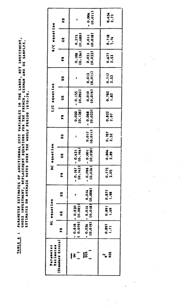
to Go Beyond the Accelerator Profits Model

One

of the theoretically most important determinants of firm factor demand

that we neglect in the accelerator profits model is the relative expected cost

of

labor and capital. If the firm anticipates that the wage rate will increase

more rapidly relatively to the user cost of capital, it will be induced to

substitute more capital for labor. Assuming the simplest (standard) assumptions

with a Cobb—Douglas production function (and constant returns), the elasticities of the relative cost of labor and capital should be in theory equal to minus the share of capital (in value added, say about —0.3) in the labor demand equation,

and to the share of labor (say 0.1) in the capital demand equation. If the pro-duction function has an elasticity of substitution between capital and labor a

(and is for example of the Constant Elasticity of Substitution form), the shares should be multiplied by a and the coefficients reduced in that proportion (say

—0.30 and 0.10 with a plausibly less than i). If the production function is of the

type "putty—clay" (the ex—ante production function for each capital vintage

being for example Cobb—Douglas),

the coefficients should also be reduced and in

quite

a large proportion (say by a factor of 10). Thus the theoretically

expected

orders of magnitude of the labor and capital costs elasticities could

be extremely different a priori, and their estimation is an empirical issue of

great import.

Despite

the considerable amount of econometric research that has been done on precisely this issue, there are still doubts and debates among economists

about the real importance of factor price elasticities. Although we could

worthwhile to explore the matter at the firm level on our data. Unfortunately, the results we get are either insignificant or dubious if significant. As usual, and probably not unfairly in the present instance, the suspicion falls

on the data.

Besides the basic problem of observing only the actual values of the variables and not their expected values, our measures of the cost of labor and capital suffer from other shortcomings. Our labor cost variable W is the average labor compensation (total wages and associated social charges) per employee. The wide dispersion in W across firms thus largely corresponds to

differences in labor qualifications, in the number of hours worked and of over-time, and only partly reflects the true differences in wages in the labor

market. Also, by construction, W will be affected by measurement errors in the

number of employees L, and this is a possible cause of a negative spurious

correlation between the two. It is also the case that W cannot be computed for the U.S. sample, since most U.S. firms declare their labor cost and material

purchases lumped together (in the item "cost of goods sold").

Our proxy for the cost of capital IR reflects only the interest rate com-ponent of a proper measure of the user cost of capital; it is computed as total

interest expenses divided by total debt. It is thus the apparent average rate

of interest paid by the firm, and in an analogous way with W it is only loosely related to the present rates of interest prevailing (at the margin for a given firm) on the financial markets.

Because of our growth rate formulation, the additional variables we enter

—28—

iR). It will be sufficient to report the estimates obtained from the 10 years average rates (the other estimates on yearly rates or on subperiods being neither better nor worse). Table 6 thus gives the estimated labor and capital cost

elasticities (and their estimated standard errors) for our four equations and three samples (in a format similar to that of Table 3). We do not reproduce the

estimated accelerator and profits effects, since the introduction of the cost

variable does not change them much from what they are in Table 3 (i.e., DW and DIR are nearly orthogonal to DQ and PR in our samples). We have been careful to

introduce DW and DIR separately in our equations without imposing a priori that

their coefficients should be equal. One reason is that only DIR is available in the U.S. sample. But more importantly, as it has been pointed out by Clark and Freeman (1980) and further developed by Dormont (1983), in this way we avoid

contaminating one variable with errors of measurement affecting the other one. The cost of capital variable is in fact extremely dispersed and suffers quite

probably from very large random errors. Hence we can expect that its estimated

elasticity is strongly biased towards 0, while the estimated labor cost elasticity might be more satisfactory.

The results in Table 6 are basically disappointing, and do not call for

long coimnents. Almost all cross price elasticities (i.e., the DW coefficient in

the investment equations and the DIR coefficient in the labor equation) are sta-tistically insignificant at the 5% level of confidence. The DW coefficient in the DC equation for Germany is an exception, but has the opposite sign

(negative) to what would be expected. It has the right sign (positive) in the

computed in the German sample. The (direct) capital cost elasticities in the investment equations are also insignificant but for the French sample. In this

case, the sign is correct (negative) but the magnitude seems small, although random errors in DIR could account for it.

The (direct) labor cost elasticities in the labor equation seem too good to be true. Their magnitude is much larger than expected (—0.8 as against —0.3

if the elasticity of substitution of capital and labor 0

is

about 1). It seems also inconsistent with the view of labor—capital substitution that the labor cost variable would show up so strongly in the labor demand, and not conversely

in the investment demand. One plausible explanation is the existence of

measurement errors in our measure DL, which by construction would be

(negatively) transmitted to our measure DW. Since the variance of DW is much

smaller thayi that of DL (by a factor of the order of 4), even relatively small

errors in DL would lead to relatively large ones in DW. Thus if random errors

were responsible for about 20% of the observed variance of DL, they could also

be responsible for as much as 80% of the observed variance of DW. Such

situation could account for our estimated elasticities of —0.8, even though the "true" coefficients would be zero.13

In closing, we should say again, if only by way of taking some comfort, that such inconclusive results in estimating price elasticities in factor demand

studies are rather common. It may be also that we have been too pessimistic in considering them. If true, this will be only a small compensation for the

—30—

IV - FINAL REMARKS

Our present work is just a step in a line or a style of research, which we think to be fruitful and deserving further effort: the analysis of

macroeconomic issues using microdata in a comparative setting. The

dif-ficulties, however, of this style of research, which combines the problems of individual data studies to those of international comparisons are equal to the

promises. Facing such difficulties, one should be specially cautious. This is why we are reluctant to put much emphasis on differences of results between

countries, even when they correspond to what could be expected, while we put a

priori more faith in finding comparable patterns of results and behavioral

similarities. Differences of results may be due, in part or even completely, to

errors or discrepancies in the data and to inadequate specifications of the

models. On the contrary, it seems implausible to obtain similar results if they

were not truly so.

Although comparative macroeconomists are usually more interested in

looking at differences between countries, it is fortunate, from what we just

say, that we find mainly similarities in our study. Despite the diversity of

situations and evolutions of French, German and US manufacturing over the period 1910—79, the labor and investment demand behaviors of large firms in the three

countries are in fact largely comparable. This is the main message of the analysis; however, this message should not be overstated. There is still room

for interesting differences; even if limited and hard to ascertain, these may be

would expect, the US firms seem to behave in a somewhat more flexible way then

their French and German counterparts, the accelerator effects tending to be higher for labor and investment and more rapid for labor in the U.S. than in the other two countries.

Among the many directions in which further work should be done, three must be mentioned here.

The problems of interpreting and specifying the accelerator and profits effects and the permanent—transitory distinction should he investigated further. It would be certainly interesting to pursue the vector autoregressive approach already used in MAIRESSE and SIll (l9R1). There are also many difficulties, however, with this approach, and unless we put complete faith in a given speci-fication, we are still in a dilemma of choosing a formulation of variables in ternis of growth rates or 1evels.l4 To make more decisive progress would probably need to have some direct notions of the firm expectations about demand and pro-fitability in both the short and long run.

More effort should be devoted to investigating the role of factor prices and to deciding whether our finding of inconclusive evidence is due to the use of poor measures, or because the effects of prices are relatively small and

there is little to discover. However, obtaining appropriate measures of labor and capital user costs at the firm level is very problematic. One might think

that there is very limited dispersion of true factor prices among firms, at

least within industries in a given country. Thus one would use the average macro—prices which can be better specified and estimated. We are not very

—32—

mation,

and we know from all the econometric research done at the macro—level

that we should foresee mixed results at best.

Specific efforts should be also devoted to the important issue of

replacement investment. There is very little work done on this issue, contrary to that of factor prices, one main reason being the lack of information. Since

balance sheet data are one of the very few possible sources of relevant

information on the subject, detailed analyses should be applied to them.15 It

would be important, for example, to try to make corrections for acquisitions, disacquisitions, and the revaluation of assets, and to be able to separate

equipment and structures for long enough periods of study. This seems indeed a

TABLE I ; MEANS AND STANDARD DEVIATIONS ( ) OF TIlE MAIN VAHIABLF.S IN THE FRENCh (N — 307), GERMAN (N — 145) ANI) US (N — 422) SAMPLES, FOR TIlE WHOLE PEKIOI) 1970—79 APIlI TUE THREE SUNPEKIOUS 1970—73, 197'.-75, 1976—79. CORRESPONDING AGGREGATE ESTIMATES FOR MANUFACTURING AS A WhOLE AS CONCERNS LABOR AND OUTPuT GROWTH RATES. VARIABLES

in

2 FRANCE 70—79 70—73 74—75 76.79 GERMANY 70—79 70—73 74—75 76—79 U.S.A. 70—79 70—73 74—15 Labor rate of growth DL 0.6 _(8.8) 3.1 _(9.7) — 0.5 (8.9) 1.3 (6.9) — 1.4 (9.7) 0,4 (10.0) — 5.2 _(2.1) — 1.4 (9.6) 1.5 (111.6) 2.4 (12.1) 3.4 (12.2) Capital rate of

OhOth7C

(10.3) (10.1) 5.1 (9.9) 1.0 (9.5) 2.0 (6.1) 4,5 _(6.2) 1.1 (4.6) — 0,2 (5.6) 6.5 (p.5) 5.7 (9.5) 3.7 (9.0) Gross invest— meat rate I/C 8.9 (8.2) $1.7 (9.4) 8.2 (7.1) 6.5 (6.4) 7,1 _(5.4) 9.1 (6.1) 5.8 (3.6) 5.6 (4.7) 8.4 (5.8) 8.8 (6.2) 8.1 (5.3) Replacement

rat.

K/C 4.3 _(7.3) 3.6 (5.6) 3.1 (7.2) 5.5 (8.6) 5.2 (2.7) 4.6 (1.7) 4.7 (2,3) 6.0 (3.4) 3.9 _(7,0) 3.0 _(6.7) 4.4 _(6.5) Sal.. rat. of growth

L

4.7 (14.0) 8.6 (12.5) — 1.4 (16.6) 3,8 (12.6) 1.8 (12.3) 4,4 (11.9) — 2.9 (13.5) 1.6 (11.4) 3.6 (12.9) 5.4 (12.5) — 4.9 ($4.0) P fIt t ro ra 19.7 (16.3) 22.3 _(16.8) 19.7 (16.0) 17.1 (15,6) I 1,0 (8.4) $3.5 (9.0) 10.1 (7.3) 9,0 _(7.S) 25,5 ($9.7) 26.8 23.4 (21.4) ($9.8) Labor produc- tivity rate of gwth (Dq-DL 4.1 5.5 — 0.9 5.1 3.2 4,0 2.3 3.0 2.1 3 0 • — 1 5 • — 6.4

Corresponding aggregate Correaponding aggregate

DL 4.0 6.3 — 0,9 4.0 2,7 4.5 — 4,2 4.4 2.3 3.2 0.1 1,9 .

_-

0.7 1.2 — 1.1 0.4 — 4.7 — 0.8 0.1 — 0.7 —

4.

-

I.)

Corrcspondj, aggregate (DQ—UL

4

-

0.2 5.2 3.8 4.1 0.5 3.6 2.2 3.9

TA1LE

'

ESTIMATES OF THE LAJIOR, NET INVESTMENT, CROSS INVESTMENT Atifi REPLACEMENT EQUATIONS FOR THE FRENCH, CER!AN AND U,. SAMPLES — ESTIMATES ON YFAKI.Y KATES I0N TilE WhOLE IlI1OhI l)7o_79 Parameter Estmatea (Standard Error.) 0 FR L equatto CE n US DC equation FR CE US I/C equaticn FR CE US k/C equation FR CE US flQ (

)

0.291 (0.011) 0.305 (0.021) 0.424 (0.013) 0.184 (0.014) 0.115 (0.012) 0.166 _(o.out) 0.101 (0.011) 0.116 _(0.011) 0.05! _(o.oni) — 0.063 _(0.010) 0.001 _(0.006) — 0.115 (0.010) flQ

)

0.091 _(0.010) 0.125 _(0.020) 0.044 _(0.012)

0.!!!

_(0.012) 0.094 _(0.011) 0.090 _(0.osi) 0.069 _(0.010) 0.095 (0.011) 0.060 _(0.007) — 0.042 (0.010) 0.00! (0.006)

-

0.030 (0.009) flQ

2)

0.038 (0.010) 0.005 (0.019) 0.020 (0.011) 0.096 _(0.012) 0.086 (0,011) 0.076 _(0.010) 0.069 (0.009) 0.078 (0.010) 0.043 (0.006)

-

0.027 (0.009)

-

0.008 (0.006)

-

0.034 (0.008) DQ — ) 0.055 (0.010) 0.008 (0.018) 0.015 (0.01!) 0.074 (0.012) 0.060 (0.010) 0.079 (0.010) 0.045 (0.009) 0.048 _(0.010) 0.042 _(0.006) — 0.029 (0.009) — 0.013 _(0.005)

-

0.037 (0.008) PR ( 1

-

0.034 (0.017) 0.017 (0.046) 0.210 (0.011) — 0.027 (0.020)

-

0.004 (0.026) 0.134 (0.010) 0.058 (0.016) — 0.009 (0.025) 0.108 (0.006) 0.085 (ó.016)

-

0.005 (0.013) — 0.026 (0.008) PR ( — ) 0.106 (0,016) 0.115 (0.044) — 0.113 (0.010) 0.172 (0.020) 0.187 (0.025) 0.043 (0,009) 0.117 _(0.016) 0.118 (0.024) 0.027 _(0.006) — 0.055 _(0.015) — 0.069 (0.013) — 0.016 (0.008) 0.285 0.200 0.419 0.208 0.333 0.286 0.248 0,256 0.318 0.063 0.149 0.090 RSE 7.42 8.66 8,87 9.20 4.96 8.02 7.12 4.67 4.82 7.09 2.50 6.72 E Iii) 0.475 0.443 0.503 0.465 0.355 0.4!! 0.284 0.337 0.196 — 0.18$ — 0.019 — 0.216 E PR 0.072 0.098 0.097 0.145 0.183 0.177 0.175 0.109 0.135 0.030 — 0.074 — 0.042 lotal AcceLerator El lect 0.525 0.498 0.626 0.572 0.461 0.630 0.425 0.399 0.36! — 0.147 — 0.061 — 0.268

TABLE 3 a ESTIMATES OF THE LAROK, NET INVESTMENT, CROSS INVESTMENT, REPLACEMENT EQUATIONS FOR THE FRENCH, GERMAN and US SAMPLES — ESTIMATES ON AVERAGE RATES OVER THE WHOLE PERIOD 1970—1979. Paraneter Eat

tates

(Standard Errors) DL equetton ER CE US DC equation FR GE US I/C equation ER GE US R/C equation ER GE DQ ) PB C ) 0.582 (0.033) 0.052 (0.011) 0.680 (0.066) 0.024 (0.039) 0.762 _(0.027) 0,042 _(0.008) 0,548 (0.051) 0.088 (0.017) 0.331 (0.091) 0.202 (0.054) 0.672 (0.03S) 0.087 (0.011) 0.349 (0.049) 0.136 (0.017) 0.326 (0.056) 0.069 (0.034) 0.349 (0.03S) 0.088 (0.011) — 0.199 _(0.048) 0.068 (0.016) — 0.005 _(0.054) — 0.13) _(0.033) k2 RSE 0.858 1.99 0.824 2.18 0.876 1.98 0.768 3,09 0.185 3.00 0.787 2.52 0.820 2.98 0.771 1.85 0.717 2.52 0.674 2.94 0.692 1.79 Total Accelerator Ettect 0.642 (0.032) 0.698 (0.059) 0.824 _(0.025) 0.650 _(0.049) 0.484 (0,085) 0.800 _(0.033) 0.518 _(0.050) 0.378 (0.051) 0.479 (0.033) .. 0.145 _(O045) — 0.106 _(0.051)

TABlE 4 ESTIMATFS OF THE (I)IKECT AND TOTAl.) ACCElERATOR FFFF.CTS AND PROFITS EFFECTS FOR TIlE lABOR, NFl' INVESTIIENT, GROSS INVESTMENT AND REI'LACEI*:NT EQUATIONS ON 11W FRENCH, GERMAN AND U S SAMPLF.S. ESTIMATES ON YEARLY AND AVERAGE RATES FOR TIlE. TWO SUIIPENIODS $970—li ANt) 1976—79, Type of Estimates Subp.riods DL EQUATION FR DC EQUATION FR GE US I/C EQUATION FR GE US I/C EQUATION FR Yearly 70—73 I DQ £ PR Tot.Ac. 0.51 0.08 0.57 0.5$ 0.08 0.56 0.57 0.08 0.67 0.40 0.18 0.56 0.36 0.21 0.48 0.41 0.18 0.64 0.32 0,20 0.50 0.38 0.15 0.47 0.21 0.13 O.R

-

0.08 0.02 — 0.05 0.02 -0.06 - 0.01

-

0.20 - 0.04 - 0.16 76—79 DQ E PR Tot.Acc. 0.41 0.10 0.47 0.32 O. 12 0.37 0,54 0.

Ii

0.67 0.33 0.11 0.40 0.33 0.07 0.36 0.46 0. 16 0,66 0.07 0.15 0.20 0.31 —0.01 0.30 0.22 0.13 0.38 — 0,25 0.04 — 0.20 — 0.02 — 0.08 —0.II6 — 0.24 — 0.03

-

(1.28 70—73 0,1'I 0.7i 0,79 0,38 0.19 0.55 0.32 0.24 0,29 0.06 0.05 — 0.26 PR 0.05 —0.03 0.04 0.13 0.25 0.10 0.16 0.17 0.09 0.03 — 11.0K — 0.01 Tot.Acc. 0.66 0,69 0.84 0.50 0.31 0.69 0.46 0.32 0.42 0.04 — 0.01 — 0.27 Average _________ ________ _______ Rates 76—79 017 0.37 0.50 0.10 O.2'j 0.24 0.44 0.10 0.18 0.22 — 0,15 — 0.06 — 0.2$ PR 0.09 0.09 0.07 0.09 0.10 0.10 0.12 -0.00 0.10 0,03

-

0. 10 0.00 Tot.Acc. 0.42 0.53 0.78 O.3I 0.27 0.56 0.18 0.18 0,34 —0.13 — O.0I — 0.22

fl!pr _{rr wo suiptios 7970-73 ANfl 7976—'9, AND : EXPLANIC THfl! CHA:CES}

Tk'IFN THE3E TWO S1.IPF"INS.

FRANCE I 70—73 76—79 GER1'.AY I I 70—73 76—79 U.S.A. I 70—73 76—79 J

.

DI. DA IA OP DCst Cit

t

5.0 0.5 0.7 0.2 —3.3 3.7 2.2 0.2 0.7 —0.2 — 4.2 — 7.3 — 2.8 — _0.3 0.0 — 0.4 —0.9 —4.4 3.0 0.1 0.2 0.2 —3.1 0.4 1.1 0.0 0.2 0.3 —3.0 — _7.4 — 1.9 — 0.1 0.0 0.1 0.7 — _1.8

4.l

0.3 0.8 0.2 —3.0 2.4 4.5 0.4 0.7 0.3 — 2.9 3.0 0.4 0.1 — 0.7 0. 1 —0.1 0.6 DC DA IA OP DCst Cit

E

4.7 0.9 7.7 — 0.5 7.8 a.o 2.1 0.4 1.1 — 7.7 — _1.5 7.0 — 2.6 — 0.5 0.0 — 0.6 — 3.3 —7.0 7.5 0.7 2.0 0.4 0.3 0.5 0.2 7.6 — _P.O — _7.5

:—;:;

— 7.0 — 0.5 — _0.4 — _7.4 — _7.8 — 3.6 0.7 1.6 — 0.2 0.0 3.7 4.0 0.8 7.4 — _1.1 — 1.4 3.7 0.4

0.)

— 0.2 0.9 — _1.4 — 2.0

j/r

DA IA OP DCst Cit 17E 3.0 7.5 7.5 0.4 5.3

ii.7

7.3 0.5 1.8 —

LI

4.0 6.3 — 7.7 — 7.0 0.3 — _7.5 — 7.3 —5.2 7.4 0.2 0.7 7.1 3.7 9.1 0.5 0.1 0.3 — _0.8 5.5 3.8 — 0.9 — 0.1 — 0.2 — _7.9 —0.2 —3.3 7.9 0.7 1.7 — 0.3 4.8 8.8 2.1 0.8 1.4 . — 0.5 4.5 8.3 0.2 0.1 —0.3 — _0.2 —0.3 — 0.5 R/C DA IA OP Dcit Cit R/C — 7.7 0,5 0.6 0.8 3.4 3.6 — 0.8 0.2 0.6 — _0.1 5.6 5.5 0.9 —_0.3

0.0

—0.9 2.2 7.9 0.0 —0.9

-

0.9 7.0 5.4 4.6 0.0 —0.4 —0.8 0.1 7.7 6.0 0.0 0.5 0.7 —0.9 7.7 1.4 — 7.7 0.0 0.0 0.0 4.7 3.0 — 1.9 0.0 0.0 0.7 5.6 4.6 — 0.2 0.0 0.0 0.7 1.1 7.6

TABLE 6 PARAMETER ESTIMATES OF ADDITIONNAL COST VARIABLES IN TIlE LAROR, NET INVESTMENT, GROSS INVESTMENT, RFPLACF.MENT EQUATIONS FOR TRY FRF.NCH, GERMAN AND US SAMPI.F.S. ESTIMATES ON AVERAGE RATES OVER TIlE WhOLE PERIOD 1970—79.

Para.et.r

Eat

Lat.s

(Standard Errors) DL •quation FR GE US DC squat ion FR GE US

I/C

equation FR GE US RIC equation FR GE US

a

OW ( ) DIR _I ) — 0.818 ( 0.079) — 0.034 _(0.019) — 0.830 _(0.085 — 0.014 _(0.018 — 0.014 _(0.008) — 0.167 (0.142) - 0.098 _(0.034) — 0.431 _(0.146) - 0.001 _(0.030) — 0.017 (0.011) 0.020 _(0.138) — 0.068 _(0.033) — 0.155 _(0.092) 0.010 _(0.019) — 0.013 _(0.011) 0.188 (0.136) 0.031 (0.033) 0.215 (0.088) 0.011 (0.018) — — 0.004 _(0.011)

2

RSE 0.897 1.71 0.891 1.69 0.877 1.98 0.715 3.05 -0.804 2.89 0.787 2,52 0.822 2.97 0.182 1.82 0.717 2.52 0.617 2.53 0.718 3.74 0.454 2.73

Appendix I — The Robustness of estimates to the measurement of of investment and capital stock

Since our measures of investment and capital stock were different in the German sample and in the two other samples, it seemed particularly useful to

investigate

the sensitivity of our estimates to the differences in these

measures. It was simplest to compute alternative measures on a strictly

com-parable

basis for all three samples. Investment was taken as the change In net

plant

plus depreciation charges (as was already the case for the German sample) and capital stock was estimated according to the standard application of the

permanent inventory method under the assumption of a constant rate of replace-ment 5. Under this assumption the distinction between replacereplace-ment and

depre-ciation (and that between net and gross capital stock) vanishes in principle.

Hence, we thought more appropriate to adopt a relatively large value for the

constant rate of l0, which makes our measure of capital stock closer to the

notion of a net capital stock, and has the practical advantage of giving less

importance to the choice of the initial benchmark capital stock. As the bench-mark capital, we took simply the reported book value of net plant at the

beginning of 1967, multiplied by what seemed an appropriate factor of

adjust-ment.

In fact, both the choice of the factor of adjustment and that of the

constant rate ô in plausible ranges have little impact on our estimates of the investment equation. Estimates of the accelerator and profits effects for the

three samples (on yearly and average growth rates over the whole period) are

given in Table Al. By comparing them to the corresponding estimates in Tables 2 and 3 in the text, it is apparent that they yield a fairly similar

—3I —

picture.

On the whole they tend to be closer to the estimates of the net

investment equation (rather than the gross investment equation) and somewhat more comparable for our three country samples.

for the French, German and US. samples. Estimates

on yearly and average rates for the whole period.

DC and I/C equation

FR GE US

Estimates on yearly rates

0.316 0.4)42 0.368

DQ

PR 0.1)48 _{0.136 0.130}

Total Accelerator Effects 0.515 0.558 0.589

Estimates on average rates

0.5)46 0.1430 0.609

DQ

E PR _{0.078 0.085}

0.071

—35—

Appendix

II —

_Estimates

of the Total Accelerator Effects

with Different Lag Specifications

As was noted in the text, before adopting a specification with three lags for

sales growth rates (and one for profit rates) we experimented with a number of

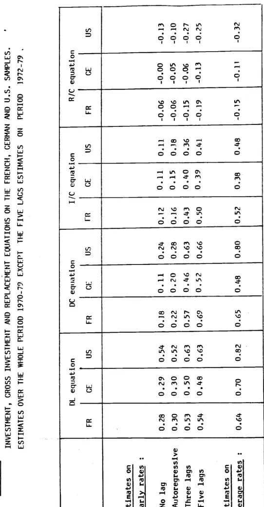
different specifications. Table A2 presents the various estimates of the total

accelerator effects obtained when using no lags (only the current value DQ),

five lags (DQ, DQ1,...DQ5) and geometrically decreasing lags in the first auto—regressive form (i.e., introducing the one lag endogenous variable, DL1 or DC1 or i/C1 or R/C1, in addition to DQ, as an explanatory variable). For the

ease of comparison, Table A2 repeats also the corresponding estimates on yearly rates with three lags (last line of Table 2) and on average growth rates (last

line of Table 3). It is generally clear that for the four equations and three

countries our three lag estimates of the total accelerator effects do not differ much from the five lags estimates, both types of estimates being sizeably larger

than the no lag estimates, and being smaller with some exceptions than the average rates estimates. It is also interesting to note that the

estimates obtained with the autoregressive specification are practically the same as the no lag estimates.

TABLE A2 : ESTIMATES OF THE TOTAL ACCELERATOR EFFECTS USING DIFFERENT LAG SPECIFICATIONS FOR THE LABOR, MET INVESTMENT, CROSS INVESTMENT AND REPLACEMENT EQUATIONS OH THE FRENCH, GERMAN AND U.S. SAMPLES. ESTIMATES OVER THE WHOLE PERIOD 1970-79 EXCEPT THE FIVE LAGS ESTIMATES ON PERIOD 1972-79 DL equation FR CE US DC equation FR CE US I/C equation FR CE US RIC FR equation GE Estimates on yearly rates

-

No lag -

Autoregressive

- Three lags -

Five

lags 0.28 0.30 0.53 0.54

0.29

0.30

0.50

0.48 0.54 0.52 0.63 0.63 0.18 0.22 0.57 0.69 0.11 0.20 0.46 0.52 0.24 0.28 0.63 0.66 0.12 0.16 0.43 0.50 0.11 0.15 0.40 0.39 0.11 0.18 0.36 0.41 -0.06 -0.06 -0.15 -O.19 -0.00 -0.05 -0.06 -0.13 Estimates on Average rates : 0.64 0.70 0.82 0.65 0.48 0.80 0.52 0.38 0.48 -0.15 -0.11