Boundary effects and repeat-sales
Arnaud Simon
Université Paris-Dauphine
CEREG
Place du Maréchal de Lattre-de-Tassigny
75775 Paris Cedex 16
Boundary effects and repeat-sales
Abstract
We study in this article the consequences of the double censoring (right and left) applied on every sample of repeat-sales before calculating a repeat-sales index. We show that, independently of the specificities of each dataset, there exist some intrinsic features for this kind of index that directly depend on the censoring mechanism. Working with the standard deviation of the estimator and the well known bias of the Cass, Shiller model we bring to fore a time structure for these two quantities. Their behaviour is different near the edges of the interval compared to the middle, and this phenomenon is generally more pronounced for the right side than for the left side. A sensitivity analysis is developed using a “neutral sample” in order to study the way this U-shape evolve in relation with the fundamental parameters. With this analysis we also try to determine the optimal length of the estimation interval, the consequences of the data dispersion and the impact of the liquidity levels in the market (number of goods sold at each date and resale speed).
1. Introduction
The two seminal articles for the repeat-sales technique are Bailey, Muth and Nourse (1963), in an homoscedastic situation, and Case, Shiller (1987) for the heteroscedasctic context. Since these two papers the repeat-sales approach has become one of the most popular index because of its quality and its flexibility. It used not only for residential but also for commercial real estate, cf. Gatzlaff, Geltner (1998). One can also refer to Chau et al. (2005) for a recent example of a multisectorial application of the RSI (repeat-sales index) and to Baroni et al. (2004) for the French context. In this article we are going to study the time structure of the errors and how the reliability of the index evolves. For any index technique the errors is generally not one single piece. We can divide the errors in two elements: the first component depends one the methodology employed and the second one depends on the specificities of each dataset. Our goal in this paper consists in studying the first one, although we will give some elements on the second one when we will study the liquidity shocks. The main characteristic of the repeat-sales technique is its double censoring mechanism. Indeed, when we work with an estimation interval [0,T], the repeat-sales with a purchase before 0 or a resale after T are not considered during the estimation process. As we will see, this feature has some important consequences on the time-structure of the errors: we will generally observe an asymmetric U-shape. With a sensitivity analysis we will try to determine which are the main intrinsic factors that drive this structure. We will study the impacts of the noises, the length of the estimation interval, the level of liquidity in the market and the resale speed. As a by-product we could give some clue about the optimal choice of parameters to estimate a RSI. For instance, the number of transactions collected for the first date seems to be a important driver of the global reliability of the index. The rest of this paper is organised as follows. Section 2 presents the repeat-sales index theory. If we want to study the structural
determinants of the errors we have to work with a “neutral sample” in order to remove the impact of the specificities of a real dataset; Section 3 presents the neutral sample. Section 4 is devoted to the sensitivity analysis. The last section will conclude.
2. The estimation of the RSI
In this paragraph we summarize briefly the theoretical framework established in Simon(2007).
2.1.
The classical estimation of the repeat-sales indexIn the repeat-sales approach, the price of a property k at time t is decomposed in three parts: Ln(pk,t) = ln(Indext) + Gk,t + Nk,t
Indext is the true index value, Gk,t is a Gaussian random walk representing the asset’s own
trend and Nk,t is a white noise associated to the market imperfections. If we denote Rate =
(rate0, rate1, …, rateT-1)’ the vector of the continuous rates for each elementary time interval
[t,t+1], we have Indext = exp(rate0 + rate1 + … + rate t-1), or equivalently ratet = ln(Indext+1
/Indext). For a repeat-sale we can write at the purchase time ti : Ln(pk,i) = ln(Indexi) + Gk,i + Nk,i
and at the resale time tj : Ln(pk,j) = ln(Indexj) + Gk,j + Nk,j. Thus, subtracting, we get Ln(pk,j/pk,i)
= Ln(Indexj/Indexi) + (Gk,j - Gk,i) + (Nk,j - Nk,i). The return rate realised for the property k is
equal to the index return rate during the same period, plus the random walk and the white noise increments. Each repeat-sale gives a relation of that nature, under a matrix form we have Y = D*LIndex + ε. Here, Y is the column vector of the log return rates realised in the estimation dataset and LIndex = ( ln(Index1), … , ln(IndexT) )’. ε is the error term and D is a
non singular matrix1. Moreover, if we notice that there exists an invertible matrix2 A, such that
LIndex = A Rate, we can also write3 Y = (DA) (A-1 LIndex) + ε = (DA) Rate + ε. In the
estimation process, the true values Index and Rate will be replaced with their estimators, respectively denoted Ind = (Ind1,… , IndT)’ and R = (r0, r1, …, rT-1)’. The usual estimation of Y
= D*LIndex + ε or Y = (DA) Rate + ε is carried out in three steps because of the heteroscedasticity of ε. Indeed, the specification of the error term leads to the relation Var(εk)
= 2σN²+ σG²(j-i) in which the values σN and σG are the volatilities associated to Gk,t and Nk,t ,
and j-i is the holding period for the kth repeat-sale. The first step consists in running an OLS
that produces a residuals series. These residuals are then regressed on a constant and on the length of the holding periods to estimate σN, σG and the variance-covariance matrix4 of ε,
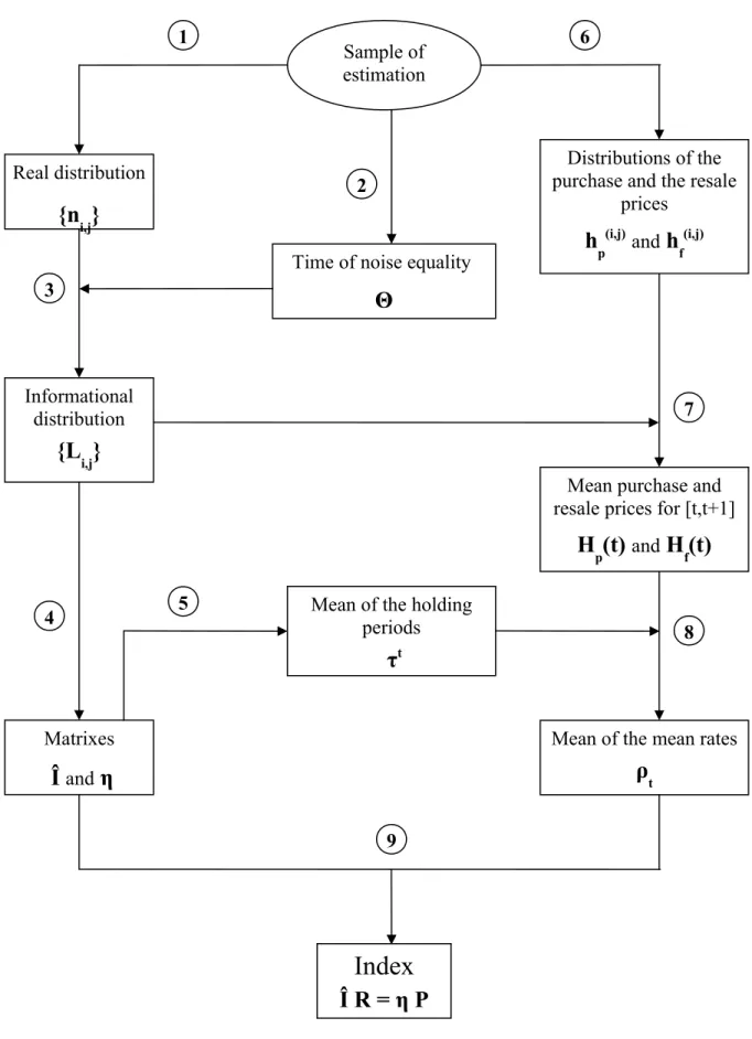
denoted Σ. Finally, the last step is an application of the generalised least squares procedure with the estimated matrix Σ. In Simon (2007) we establish that this traditional approach is equivalent to an algorithmic decomposition (cf. Figure 1), where the informational framework becomes explicit. The next paragraphs present briefly the mechanism of this algorithm.
2.2.
Notations, basic concepts and decomposition of the RSI1.1.1. Time of noise equality
The variance of the residual εk measures the quality of the approximation Ln(pk,j/pk,i) ≈
Ln(Indj/Indi) for the kth repeat-sale . This quantity 2σN² + σG²(j-i) can be interpreted as a noise 1 D is a matrix extracted from another matrix D’; the first column has been removed to avoid a singularity in the estimation process. The number of lines of D’ is equal to the total number of the repeat-sales in the dataset and its T+1 columns correspond to the different possible times for the trades. In each line -1 indicates the purchase date, +1 the resale date and the rest is completed with zeros.
2 A is a triangular matrix whose values are equal to 1 on the diagonal and under it, 0 elsewhere.
3 The basic rules of linear algebra indicate that the matrix DA gets as many lines as the number of repeat sales in the sample, and that the columns correspond to the elementary time intervals. In each line of DA, if the purchase occurs at ti and the resale at tj, we have ( 0 … 0 1(ti) 1 … 1(tj-1) 0 … 0). Therefore, the relation Y = (DA) Rate + ε simply means that Log(return) = ratei+ … + ratej-1+ ε
measure for each data. As a repeat-sale is composed of two transactions (a purchase and a resale), the first noise source Nk,t appears twice with 2σN². The contribution of the second
source Gk,t depends on the time elapsed between these two transactions : σG²(j-i).
Consequently, as time goes by, the above approximation becomes less and less reliable. For the future developments it is useful to modify slightly the expression of the total noise, factorising by σG² : 2σN²+σG²(j-i) = σG²[(2σN²/σG²)+(j-i)] = σG²[Θ+(j-i)]. What does Θ =
2σN²/σG² represent? The first noise source provides a constant intensity (2σN²) whereas the size
of the second is time-varying (σG²(j-i)). For a short holding period the first one is louder than
the second. But as the former is constant and the latter is increasing regularly with the length of the holding period, there exists a duration where the two sources will reach the same levels. Then, the Gaussian noise Gk,t will exceed the white noise. This time is the solution of the
equation: 2σN² = σG² * time time = 2σN²/ σG² = Θ. For that reason, we will call Θ the “time
of noise equality”. Below in the formula, the function G(x) = x/(x+Θ) will sometimes appear. For an holding period j-i we have G( j – i ) = (j-i)/(Θ+(j-i)) = σG²(j-i)/[2σN²+σG²(j-i)]. G(j-i) is
the proportion of the time-varying noise in the total noise; these numbers will be used subsequently as a system of weights.
1.1.2. Quantity of information delivered by a repeat-sale
The theoretical reformulation developed in this article brings the concept of information at crucial place. As Θ+(j-i) is a noise measure, its inverse can be interpreted as an information measure. Indeed, if the noise is growing, that is if the approximation Ln(pk,j/pk,i) ≈
Ln(Indj/Indi) is becoming less reliable, the inverse of Θ + ( j – i ) is decreasing. Consequently,
(Θ+(j-i))-1 is a direct measure5 (for a repeat-sale with a purchase at t
i and a resale at tj) of the
5 These measures are relative ones. The matter is their relative sizes and not the absolute levels. They can be defined up to a constant in order to standardize the measures.
quality of the approximation or, equivalently, of the quantity of information delivered. In the estimation process, the small weights for the long holding periods make these observations less contributive to the index values.
1.1.3. Subsets and algorithmic decomposition of the RSI
The set of the repeat-sales with a purchase at ti and a resale at tj will be denoted by C(i,j). For
a time interval [t’,t], we will say that an observation is relevant if its holding period includes [t’,t] ; that is if the purchase is at ti ≤ t’ and the resale at tj ≥ t. This sub-sample will be denoted
Spl[t’,t]. For an elementary time-interval [t,t+1], we will also used the simplified notation
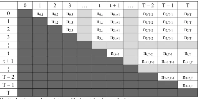
Spl[t,t+1] = Splt. If we organize the dataset in an triangular upper table, the sub-set Spl[t’,t] will
correspond to the cells indicated in Table 1. From the optimization problem associated to the general least squares procedure, we demonstrated in Simon (2007) that the repeat-sales index estimation could be realised using the algorithmic decomposition presented in Figure 1. The left-hand side is related to the informational concepts (for example the matrix Î), whereas the right-hand side is associated to the price measures (for example the mean of the mean rates ρt). The final values of the index come from the confrontation of these two parts.
2.3.
The real distribution and its informational equivalentThe time is discretized from 0 to T (the present), and divided in T sub-intervals.
0 1 2 … t t + 1 … T - 1 T
We assume that the transactions occur only at these moments, and not between two dates (the step can be for example a month or a quarter, depending on the data quality). Each
observation gives a time couple (ti;tj) with 0 ≤ ti < tj ≤ T ; thus we have ½T*(T+1) possibilities
for the holding periods. The number of elements in C(i,j) is ni,j,and we denote N = ∑i<jnij the
total number of the repeat-sales in the dataset. Table 2a is a representation of the real distribution of the {nij}. As each element of C(i,j) provides a quantity of information equal to
(Θ+(j-i))-1, the total informational contribution of the n
i,j observations of C(i,j) is ni,j (Θ+(j-i))-1
= ni,j /( Θ + ( j – i )) = Li, j. Therefore, from the real distribution {ni,j} we get the informational
distribution {Li,j} (cf. Table 2b), just dividing its elements by Θ+(j-i). The total quantity of
information embedded in a dataset is: I = ∑i<jLij.
2.4.
Averages for the noise proportions, the periods and the frequenciesThe number of repeat-sales in Splt is nt = ∑
i ≤ t < jni,j. For an element of C(i,j), the length of the
holding period is j – i. Using the function G, we can define the G-mean6 ζt of these lengths in
Splt by ∑
i ≤ t < j ∑k’ G(j-i) = nt G(ζt). The first sum enumerates all the classes C(i,j) that belong
to Splt, the second all the elements in each of these classes. Moreover, as G(j-i) measures the
proportion of the time varying-noise Gk,t in the total noise for a repeat-sales of C(i,j), the
quantity G(ζt) can also be interpreted as the mean proportion of this Gaussian noise in the
global one, for the whole sub-sample Splt. In the same spirit, we define the arithmetic average
Ft of the holding frequencies 1/( j – i ), weighted by the G( j – i ), in Splt: Ft = ( nt G(ζt) )-1 ∑ i
≤ t < j∑k’G(j-i)*( 1 /(j-i) ) = It / (nt G(ζt)) . Its inverse τt = (Ft )-1 is then the harmonic average7 of
the holding periods j-i, weighted by the G(j-i), in Splt. If at first sight the two averages ζt and τt
6 We recall here that the concept of average is a very general one. If a function G is strictly increasing or decreasing the G-mean of the numbers {x1 , x2 , … , xn}, weighted by the (α1 , α2 , … , αn), is the number X such that: αG(X) = α1G(x1) + α2G(x2) +…+ αnG(xn) with α = ∑i=1,...,nαi. An arithmetic mean corresponds to G(x) = x, a geometric one to G(x)= ln(x) and the harmonic average to G(x) = 1/x
7 We have ( nt G(ζ t) ) / τt = ∑
can appear as two different concepts, in fact it is nothing of the sort. We always have, for each sub-sample Splt, ζt = τt.
2.5.
Two matrixesThe matrix η is a diagonal one, its T diagonal coefficients are: n0G(ζ0) , … , nT-1G(ζT-1). The ith
element gives the number of repeat-sales relevant for [i,i+1], multiplied by G(ζi). Now we are
working with the interval [t’,t+1]. A repeat-sale provides information on it if the purchase is at t’ or before and if the resale takes place at t+1 or after. The quantity of information relevant for [t’,t+1] is thus I[t’,t+1] = ∑
i ≤ t’ ≤ t < jLi,j . For an interval [t,t+1] we simply denote It for I[t,t+1].
As exemplified in Table 3, I[t’,t+1] can be calculated buy-side with the partial sums B
0t , B1t ,
… , Bt
t’ or sell-side with St’T, St’T-1, … , St’t+1. But we always have I[t’,t+1] = B0t + … + Btt’ = St’T
+ … + St’
t+1. For all the intervals included in [0,T] we get this way the related quantities of
information. These values are arranged in a symmetric matrix Î.
I[0,1] I[0,2] I[0,3] … I [0,T] I [0,2] I[1,2] I[1,3] I[1,T] I[0,3] I[1,3] I[2,3] I[2,T] ¦ I[0,T] I[1,T] I[2,T] I[T-1,T]
2.6.
The mean pricesWithin each repeat-sales class C(i,j), we calculate the geometric and equally weighted averages of the purchase prices: hp(i,j) = (Πk’ pk’,i)1/ni,j , and of the resale prices: hf(i,j) =
(Πk’pk’,j)1/ni,j. For an elementary time-interval [t,t+1], the relevant classes C(i,j) are the ones that
satisfy to the inequalities i ≤ t < j. With these classes, we calculate the geometric average Hp(t)
of the hp(i,j), weighted by their corresponding Li,j (here, the total mass of the weights is It = ∑i≤t< jLi,j):
Hp(t) = ( Πi ≤ t < j(hp(i,j)) L
i,j )1/It = ( Πi ≤ t < j(Πk’pk’,i)1 /( Θ + (j-i))
)
1 / ItAs indicated in the second part, Hp(t) is also the geometric mean of the purchase prices,
weighted by their informational contribution 1/(Θ+(j-i)), for the investors who owned real estate during at least [t,t+1]. Similarly, we also define the mean resale price Hf(t):
Hf(t) = ( Πi ≤ t < j(hf(i,j))Li,j )1/It = ( Πi ≤ t < j(Πk’pk’,j)1 /(Θ + ( j - i ))
)
1 / ItAs we can see, Hp(t) can be interpreted as a mean purchase price weighted by the
informational activity, buy-side, of the market. The interpretation is the same for Hf(t) with
the informational activity of the market, sell-side.
2.7.
The mean of the mean ratesFor a given repeat-sales k’ in C(i,j), with a purchase price pk’,i and a resale price pk’,j , the mean
continuous rate realised on its holding period j-i is rk'(i,j) = ln(pk’,j /pk’,i) / (j-i). In the subset Splt,
we calculate the arithmetic mean of these mean rates rk'(i,j), weighted8 by the G(j-i) : ρt =
(ntG(ζt))-1∑
i≤t<j∑k’G(j-i)rk'(i,j). This value is a measure of the mean profitability of the investment
for the people who owned real estate during [t,t+1], independently of the length of their holding period. The weights in this average depend on the informational contribution of each data. We demonstrated in Simon (2007) that we can also write ρt in a simpler way with the
following formula: ρt = ( 1/ τt ) * ( ln Hf(t) – ln Hp(t)). For Splt, this relation is actually the
aggregated equivalent of rk'(i,j) = ln(pk’,j /pk’,i) / (j-i), with the harmonic mean of the holding 8 The total mass of these weights is ntG(ζt)
periods τt, the mean purchase price H
p(t) and the mean resale price Hf(t). All these averages
are weighted by the informational activity of the market. We denote the vector of these mean rates P = (ρ0, ρ1, …, ρT-1).
2.8.
The index and the relation Î R = η PThe estimation of the RSI can now be realised just solving the equation: Î R = η P R = (Î-1η)P. The unknown is the vector R = (r
0, r1, …, rT-1)’ of the monoperiodic growth rates of the
index. The three others components of this equation (Î, η and P) are calculated directly from the dataset. The main advantages of this formalism are its interpretability and its flexibility: the matrix Î gives us the informational structure of the dataset, the matrix η counts the relevant repeat-sales for each time interval [t,t+1] and the vector P indicates the levels of profitability of the investment for the people who owned real estate at the different dates.
3. The exponential benchmark
3.1.
HypothesesA repeat-sales sample is never an intuitive object because of the left censoring at 0 and the right censoring at T. These cuts generate a lower data density near the edges, whereas the
quantity of information is higher in the middle of the interval. In this situation, what does a uniform distribution of repeat-sales look like? The answer is probably not unique. The benchmark sample we study in this article is based on the two following assumptions: 1) The quantities of goods traded on the market at each date are constant and denoted K. 2) The length of the holding period is deterministic. The survival curve for each cohort is an
exponential with a parameter λ > 0 (the same for all cohorts): S(t) = K e-λt.
This last hypothesis means that the resale intensity is constant. Such a choice is of course unrealistic because it implies that the percentage of sold houses in the next year is not influenced by the length of the holding period. In a probabilistic context, if we introduce the hazard rate9 which measures the instantaneous probability of resale: λ(t) = (1/Δt)*Prob(resale
> t+Δt
|
resale ≥ t), it is a well-known fact that the choice of an exponential distribution is equivalent to the choice of a constant hazard rate. In the real world things are of course different. For the standard owner (cf. Figure 2) we can reasonably think that the hazard rate is first low (quick resales are scarce). In a second time, it increases progressively up to a stationary level, potentially modified by the economic context (residential time). Then, as time goes by, the possibility of moving due to the retirement, or even the death of the householder, would bring the hazard rate to a higher level (ageing). Nevertheless, the aim of our benchmark does not consist in describing exactly the reality. We just try to modelize a basic, uniform and deterministic behaviour in order to have some comparative elements. Under these assumptions we study below the various building blocks that appear in the RSI decomposition.3.2.
The real and the informational distributions9 λ(t) is a classical concept in the survival models, cf. Kalbfleisch, Prentice (2002). It appears for example in the econometrical studies for the prepayment and the default options embedded in the mortgages, cf. Deng, Quigley, Van Order (2000).
1.1.4. Notations
We denote α = e – λ the instantaneous survival rate10; that is the proportion of goods that are not
sold during one period of time. As λ ≈ 0+ we have α ≈ 1 – λ. After k periods of time, the
disappearance rate is d(k) = 1 – αk. Thus, the mean linear disappearance rate per time unit is
λlin = d(k)/k. These concepts are illustrated with Figure 3. K represents the number of goods
traded on the market at each date. In the next paragraph the quantity K’ = K (1-α)/α will sometimes appear. If we use the approximation α ≈ 1 - λ, we get K’ = K (1 - e-λ)/e-λ = K (eλ -1)
≈ Kλ ≈ K(1-α). K’ is approximately equal to the number of resales observed in the next period within a sample of K initial elements.
1.1.5. The real distribution
We consider the K goods purchased at time i on the market. The number of goods that are still alive11 at time i+1 is Kα, at time i+2 we have Kα2,…, and at time j it remains K αj-i. From this
we get ni,i+1 = K – Kα = K (1-α) = [ K (1- α)/α ] α = K’α, ni,i+2 = Kα – Kα² = K α (1-α) = K’α²
and more generally ni,j = Kαj-i-1 – K αj-i = K’αj-i. The real distribution for the benchmark sample
is illustrated in Table 4a. The sums bi (on the lines) give the number of repeat-sales with a
purchase at i, whereas the sums sj (on the columns) give the number of repeat-sales with a
resale at j. As we have geometric progressions, we get very easily the closed formulas for these two quantities. Moreover, we can establish that the total number of repeat-sales observed with this benchmark sample is: N = KT [ 1 – α λlin(T) / (1-α)] ≈ KT [ 1 – λlin(T)/λ ].
Among the K goods traded on the market at each date, some of them will not give a repeat-sales observation because the resale will occur after T. During the time interval [0,T], as K goods are purchased at each date t (t = 0,…,T-1) we have a potential number of repeat-sales
10 We have α = S(t+1)/S(t) = S(t’+1)/S(t’) for all t and t’ 11 Here the “death” means a resale
that is equal to KT. If we compare KT and the expression that we got for N, we can establish directly that the proportion of the missing goods is simply equal to π(T) = λlin(T)α/(1-α) ≈
λlin(T)/λ. (cf. appendix A for the details).
1.1.6. The informational distribution
The ni,j elements of C(i,j) provide a quantity of information12 Li,j = ni,j / (Θ+(j-i)). Table 4b
illustrates this distribution. The informational sums on the lines Bi and on the columns Sj
depends on the values un = α /( Θ + 1 ) + α² /( Θ + 2 ) + α3 /( Θ + 3 ) +… + αn /( Θ + n ). This
number represents the quantity of information provided by a sample with K = 1/λ repeat-sales, initiated at time t, and observed during n periods of time. We denote ℓ the limit of (un) ; if we
approximate Θ with the closer integer we have ℓ = – [ln (1– α) + α + α² / 2 … + α Θ/ Θ ] / αΘ.
The total quantity of information provided by these N repeat-sales is equal to: I = K’ [ ( T + Θ + 1 ) uT – T π(T) ], cf. appendix A. If we would not have any limit of observation on the right
of the interval [0,T], the repeat-sales initiated between 0 and T-1 would provide a quantity of information equal to K’Tℓ. We establish in appendix A that the proportion of the missing information μ = ( K’T ℓ - I ) / K’T ℓ, that is the informational equivalent of π, is equal to μ = [ ℓ + π(T) – ( T + Θ + 1 ) ( uT / T )] / ℓ.
3.3.
Informational matrix and other quantities1.1.7. nt and n[t’,t+1]
nt = ∑
i ≤ t < jni, j is the number of repeat-sales relevant for [t,t+1] and n[t’,t+1] = ∑i ≤ t’ ≤ t < jni, j gives
the number of repeat-sales relevant for [t’,t+1]. With the classical formula for the geometric
progression we establish immediately that nt = ( K / (1 – α ) ) * d ( T– t ) d( t + 1) and n[t’,t+1] =
(K /(1 – α )) * ( 1 – d (t – t’) ) d(T– t) d(t’ + 1).
1.1.8. It and I[t’,t+1]
We introduce for -1 ≤ m ≤ n the notation U(m,n) = un – um = αm+1 /(Θ+m+1) + …+ αn /(Θ+n)
with the conventions u0 = 0 and u1 = -1/Θ. Moreover we denote for 0 ≤ t’ ≤ t < T:
U(t’,t,T) = (1+Θ/2)U(t,T) - [(t+Θ/2)U(t-t’-1,t) - (t’-Θ/2)U(t-t’-1,T-t’-1)] + (T+Θ/2)U(T-t’-1,T) With these notations we establish in the appendixes B and C that the formulas for It and I[t’,t+1]
are similar. More precisely we have:
I[t’,t+1] = ((1-α)/α) [ n[t’,t+1] + K U (t’, t, T) ] It = I[t,t+1] = ((1-α)/α) [ nt + K U(t, t, T) ]
We can now directly compute the informational matrix Î with these two expressions.
4.
Boundary effects and sensitivity
4.1.
The problemThe aim of this section consists in analyzing the non-uniform behavior of the RSI across time. Indeed, as we will see several of its characteristics have a time structure; the behavior near the edges is generally different of the one observed in the middle of the interval. We are going to study this point for two specific aspects:
- The standard error13 of the estimator Indt (actually, we will work with the quantity
100*σ(Indt)/Indext that gives the standard error as a percentage of the true value) 13 We recall here that Ind
t ~ LN ( Lindext ; diagt[V(Lind)] ), where V (LInd) = σG² A Î-1A’. A is a triangular matrix whose values are equal to 1 on the principal diagonal and under it, 0 elsewhere (cf. Simon(2007)). Thus we have : σ(Indt)/Indext = exp(2*Lindext + diagt[V(Lind)])0,5 (exp(diagt[V(Lind)]) -1)0,5 / Indext
- The multiplicative bias of the index14 (in percentages)
When we measure these two quantities the results of course depends of each dataset. Bur what we claim here is that, even if we take a “neutral sample”, we can observe some features that do not depend on the nature of the observations but rather than on the intrinsic characteristics of the model. The exponential benchmark developed in the section above will be our “neutral sample”. Its real distribution is known as soon as we know K and λ. In order to apply the various informational formulas, we also need to choose the values of T, θ and σG. We
introduce here a reference situation15 that corresponds to: T = 30, σ
G² = 0,001, θ = 10, K =
200, λ = 0.1. In the next paragraphs we are going to study the time structure for the bias and the variance of the estimators modifying each parameter separately for our reference.
4.2.
Time structure and sensitivity to the error terms σG and θIn the Figures 4a and 4b the reference corresponds to σG² = 0,001. The two curves (error and
bias) present a U-shape. The values on the left of the interval are a little bit higher than the ones in the middle but the edge effect is more pronounced for the right side. For the sensitivity analysis we choose to let the parameter σG² varies between 0,0001 and 0,0025. The
first extreme case means that the random-walk is small, that is we are close to the Bailey, Muth and Nourse (BMN) model. In this situation the boundary effects are small; they could even be neglected. In the second extreme case, the idiosyncratic components modelled by the random walk, are strong. As we can see the impact of σG on the errors is important (it doubles
for σG² = 0,0025 compared to the reference). The heterogeneity of the price movements in a 14 It is a well-known fact that the RSI is slightly biased (Goetzmann 1992; Goetzmann and Peng 2002). With our notations the multiplicative bias is equal to: exp( ½diagt[V(Lind)] ). We multiply this quantity by 100 to get a percentage. (cf. Simon 2007 for the details).
15 T = 30 : it corresponds to an index estimated on thirty years annually, or fifteen years on a six month basis. The level chosen for the values σG² and θ are quite standard if we refer for instance to the article Case, Shiller (1987). This value of λ corresponds to a mean holding period of ten years, and with this choice of K = 200 we have approximately N = 4100 repeat-sales in the sample.
city has some consequences for the quality of the index. In the Case-Shiller context the U-shape becomes stronger when the heterogeneity increases; this phenomenon is very clear for the bias. Regarding the parameter θ = 2σN²/ σG² it allows studying the impact of the white
noise σN² (we let σG² at its base level 0,001). When σN² varies its impact has the same
magnitude than the one generated by a variation of the random-walk (Figures 5a and 5b). If the white noise is stronger the bias and the errors evolve in the same direction (upward). Globally we also find the U-shape but a small difference appears when θ (that is σN) is close
to zero. This choice of parameter means that the white noise can be neglected and that the error term in the regression is mainly directed by the idiosyncratic component. If the Case, Shiller situation is in the middle, if the BMN context is a pole, then θ ≈ 0+ corresponds to the
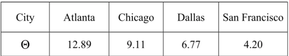
second polar situation. Here, it seems that the left boundary-effect is reversed. For instance for θ = 1 the errors and the bias are smaller for the beginning of the interval. The pivot is at θ = 5. In the article of Case, Shiller (1987) it approximately corresponds to the city of San Francisco (cf. Table 6). For the right side we do not find the same phenomenon for the small values of θ.
4.3.
Time structure and sensitivity to the length of the estimation interval TFigures 6a and 6b present the result when the time horizon is varying from T = 5 to T = 50. Here also we have a time-structure. For the short intervals ( T = 5 and T = 10) we find an additional error and an additional bias. From T = 15 the first values seem to reach their asymptotic levels. Building a repeat-sales index on a too short interval is not always reliable; as we can see the bias can double in this kind of situation. The U-shape is always there, with a greater magnitude for the right side for all the classical situations (T ≥ 15). We could have thought that the only problem with respect to the length of the time interval would have appeared for the small intervals; however it is not completely true. Indeed, for the long
interval the errors and the bias for the more recent dates increase slightly. This phenomenon appears after T = 40. Consequently, our results suggest that there exist an optimal length for the estimation interval (at least under the errors and the bias point of view). For our base situation this optimal value is approximately T = 30.
4.4.
Time structure and sensitivity to the size of the sample : K and λIn this section we study the time-structure in relation to the size of the sample. With the neutral exponential dataset the number of repeat-sales is a function of two parameters: K and λ. The first one is a measure of the volume traded globally on the market at each date16 and
the second one is associated to the length of the holding period. If K increases, or λ decreases, the number of repeat-sales is higher. Table 7a and 7b give the size of the samples when each parameter is modified separately from the base. The results for the errors and the bias are illustrated with Figures 7a, 7b for K, and Figures 8a, 8bfor λ. What is the minimal volume of transactions required to build a reliable RSI? With our base situation (T = 30, σG² = 0,001, θ =
10 , λ = 0.1) it seems that K = 50 is acceptable. With this choice the standard-error of the estimators is approximately 2,5% and the bias is small. The associated sample size is N = 1025. If we divide N by the number of dates we get: 1025/30 ≈ 34. The repeat-sales index is acceptable if we have on average 34 repeat-sales data for each date, or equivalently if we work on a market in which we can observe 50 simple transactions at each date. This low level indicates that the RSI can be reasonably computed for a very narrow market, contrary to hedonic index that requires a bigger dataset. For K = 10 and N = 205, the limit is reached; the errors become important (6%) and the bias also. If we want to a greater accuracy (for instance 1% for the errors) we would need approximately K = 300, that is N ≈ 5000 pairs. As we can
16 We recall here that only a part of the N = KT transactions provide observable repeat-sales; the missing part is given by the formula π(T) = λlin(T)α/(1-α) ≈ λlin(T)/λ (cf. 3.2.2).
see with all these simulations the bias stays at a very acceptable level, the main criterion for the analysis is actually the size of the errors. Concerning the time-structure, the results do not depend on K; the U-shape stays unchanged whatever be the value of this parameter. We are now going to examine the impact of λ. As the resale decision is exponentially distributed, the mean holding period is equal to 1/λ (10 units of time for the base). λ is a measure of the turnover rate and it seems that there exists an optimal level for this value. In Figures 8a and 8b the errors and the bias hit a low threshold for λ between 0.1 and 0.2; that is for a mean holding period between 5 and 10 units of time. For the base, if the turnover rate becomes lower, it deteriorates the quality of the index. On the other hand, a sample with very short holding periods is not really an advantage. Indeed, as we can see for λ = 0.5, the errors surprisingly increases. This type of goods, called “flips” by Clapp and Giaccotto (1999), produces higher errors and higher bias. Moreover the time structure changes, the U-shape disappears and it is replaced with an increasing line. The edge effect becomes small on the left and much more important on the right side. This result confirms once more that the flips are a very specific category. Here we demonstrated that this result holds not only because of a specific price dynamic as in Clapp and Giaccotto (1999), but also because of a structural issue related to the econometrical properties of the RSI.
4.5.
Liquidity shocksIn the previous paragraph the liquidity shock is global; it acts on the full range on the interval. We are now going to consider time-localized shocks. With the exponential benchmark we assumed that at each date K goods were negotiated on the market (t = 0,…, T-1). In order to deepen the analysis we distinguish these quantities denoting K0,…,KT-1 the volumes for these
dates. Similarly, the resale intensity at t, that is the instantaneous resale rate for the goods still alive after t -1, is denoted λt (for t = 1,…,T). We assume that the same rate λt is applied to all
the goods alive after t – 1, whatever be their initial purchase date17. Globally, the K
t and the λt
will stay at the same levels than for the reference situation. A liquidity shock just consists in a variation of a few Kt or a few λt. A change of Kt means that the volume traded on the market
at t is smaller or greater (Kt = 100 or Kt = 400, the level of the reference is K = 200). A
variation of λt means a change in the length of the holding period: a decrease of λt is
associated to a lengthening of the period and reciprocally (the shocks correspond to λt = 0,2
and λt = 0,05, the level of reference being λt = 0,1). We consider three kinds of shocks: on a
single date, on a small sub-interval in the middle of the global interval, on the right or left half-interval. For each situation, we calculate the percentages of variation for the biases and for the errors between the exponential benchmark and the shocked sample. Results are presented in the Figures 9, 10, 11, 12, 13.
1.1.9. Shock on a single date
The Figures 9 give the results when the shock (upward or downward) concerns K0, K15 and
K29. For all the dates between t = 1 and t = 29 the results are very intuitive and similar to the
ones obtained for K15 and K29; we just observe higher biases and higher errors when Kt
decreases (and inversely when it increases the biases and the errors become smaller) for the date t. This effect is more pronounced for the first dates (t = 1, 2, 3), then it decreases progressively: the impact is at the lowest level for t = 29. However, there is a notable exception for K0. The volume negotiated on the market at the first date seems to be the main
factor. Indeed, if we observe some moderate variations for Kt when t > 0, the things change 17 Indeed, we could imagine some more sophisticated shocks. For instance the resale intensity could depend on the cohort, that is the purchase date i : λt,i
drastically for t = 0. Not only the impact on the errors and on the bias at t = 0 is more important but this type of shock also affects the subsequent dates, in a very significant proportion. This strong boundary effect on the left side should invite to choose very carefully the first date when estimating an index. A bad choice, that is a date with a low level of transaction, could easily increase the bias and the error by 100% on the whole interval. The Figures 10 present the variations when the shock concerns λ1, λ14 and λ30. The effect is
globally higher when it concerns the most recent dates. But we do not observe the same kind of boundary effect than the one we have for K0; the effect simply stays localized on the
shocked date.
1.1.10. Shock on a sub-interval
Figures 11 present the effects of two shocks for four joint dates in the middle of the estimation interval. These shocks are only downward; they reduce the size of the sample. When the change affects the liquidity levels on the market Kt, the errors and the bias for the previous
date are not modified. The effect is maximal for the shocked dates, but this perturbation also deteriorates the quality of the index for the rest of the interval. If we now study a shock on the resale rate λt, it also appears at its maximal level for the modified dates. But surprisingly the
effect is quite null after the shock, or even slightly negative: improvement of the index quality… For the dates before the shock, we also obtain a quite counter-intuitive result: a shock on λt that takes place after t = 12 deteriorates the quality of the index before t = 12…
The Figures 12 and 13 correspond to various shocks on a semi-interval, separately with Kt and
λt, and in a sense that decreases the size of the dataset (Kt lower, λt higher). The first case is
quite specific; it is mainly a consequence of the shock on K0. The effect is maximal on the
shocked period but it also acts after. We can also note that the variations on the left side are exactly at the same level. With the second case (Kt = 100 for t > 15) we simply observe a
variation on the shocked part. For the third and the fourth case (shock on the length of the holding period), the effect is maximal for the modified dates but surprisingly we also observe some modifications before and after...
5. Conclusion
The reliability of the RSI is generally an asymmetric U-shape; the estimation is more accurate in the middle of the interval compared with the edges and the left side usually provides a better estimation compared with the right side. We studied the impact of various parameters that do not depend on the specificities of each dataset but are rather some intrinsic features of the repeat-sales model. We found that in a BMN context the boundary effect is smaller, or even null. At the opposite side of the range, that is when we just have a random walk without the white noise for the residuals, we found an increasing shape: the left side provides the better estimators. Between these two poles, the classical Case-Shiller model generates an asymmetric U-shape. When we looked at the length of the estimation interval we found that a short interval creates higher errors and an increasing framework. Then, an optimal level appears with the U-shape. Surprisingly, the large intervals are not the better ones. With the liquidity level and the resale speed we found that high levels of liquidity and quick resales produce the best situations. With a notable exception when the resale intensity is very high
(flips). Indeed, in this situation the framework evolves from the asymmetric U-shape to an increasing curve and the reliability of the index globally becomes lower. This result speaks for a distinct treatment of the flips. With the sensitivity analysis developed in this paper we can define what an optimal situation is: small noises (σG and σN), length of the interval around 30,
at least 50 transactions observed at each dates, a first date with the highest possible level of transaction. Some parameters matter more than others. The most important are the liquidity levels and the resale speeds. Then, we have the length of the interval, and finally the noises.
References
Bailey, Muth, and Nourse. 1963. A Regression Method for Real Estate Price Index Construction. Journal of the American Statistical Association 58.
Baroni, Barthélémy, Mokrane. 2004. “Physical real estate : A Paris repeat sales residential index”. ESSEC Working paper DR 04007, ESSEC Research Center, ESSEC Business School
Case and Shiller. 1987. Prices of Single Family Homes since 1970: New Indexes for Four Cities. New England Economic Review September/October: 45-56.
Chau, Wong, Yiu, Leung. 2005. "Real estate price indices in Hong-Kong" Journal of real
estate literature 13(3) : 337-356
Clapp, Giaccotto. 1999. “Revisions in repeat-sales price indexes: Here today, gone tomorrow?” Real estate economics 27(1) : 79-104
Deng, Quigley, Van Order. 2000. “Mortgage terminations, heterogeneity and the exercise of mortgage options”. Econometrica 68(2) : 275-308
Gatzlaff, Geltner. 1998. "A repeat-sales transaction-based index of commercial property" A
study for the real estate research institute
Goetzmann. 1992. The Accuracy of Real Estate Indices: Repeat Sales Estimators. Journal of
Goetzmann, Peng. 2002. The Bias of the RSR Estimator and the Accuracy of Some Alternatives. Real Estate Economics 30(1): 13-39.
Kalbfleisch, Prentice. 2002. “The Statistical Analysis of Failure Time Data”
Wiley-Interscience
Appendix A : Formulas for the real distribution
bi = K’α + K’α2 + … + K’αT-i = K’α ( 1 – αT-i )/(1 – α) = K ( 1 – αT-i ) = K d(T-i)
sj = K’α + K’α2 + … + K’αj = K’α ( 1 – αj )/(1 – α) = K ( 1 – αj ) = K d(j)
N = b0 + … + bT-1 = K ( d(1) + … + d(T) ) = K ( T – ( α + … + αT ) ) = K ( T – α(1-αT)/(1-α))
N = KT ( 1 – λlin(T) α/(1-α) ) ≈ KT [ 1 – λlin(T)/λ ]
π = (KT – N) / KT = λlin(T) α/(1-α) ≈ λlin(T)/λ
I = K’ ∑k = 1,…,T [( T – k + 1 ) / ( Θ + k ) ] α k (sum on the diagonals)
= K’ ( T + Θ + 1 ) ∑k = 1,…,T αk / ( Θ + k ) – K’ ∑k = 1,…,T αk = K’ ( T + Θ + 1 ) uT – K’ (α /( 1 – α )) * ( 1 – αT ) = K’ [ ( T + Θ + 1 ) uT – T π(T) ] μ = ( K’T ℓ - I ) / K’T ℓ = [ T ℓ – ( T + Θ + 1 ) uT + T π(T) ] / T ℓ = [ ℓ + π(T) – ( T + Θ + 1 ) ( uT / T )] / ℓ
Appendix B: Formula for I[t’,t+1] with t’ < t
In Figure 5a,I[t’,t+1] corresponds to the sum of the L
i,j within the area D. We know that the sum
of the Li,j on the area A + B + C + D is equal to I = K’ [ ( T + Θ + 1 ) uT – T π(T) ]. As the
areas C, A + C, B + C are triangular they are similar to the total area I. Consequently we get very easily the expressions for the sums of the Li,j on these areas just adapting the formula for
I. Now, if we notice that D = I – ( A + C ) – (B + C) + C, we get for I[t’,t+1]:
I[t’,t+1] = K’ ( (T+Θ+1) u
T – (α / (1 – α)) * ( 1 – αT ) )
– K’ ( (t+Θ+1) ut – (α / (1 – α)) * ( 1 – αt ) )
– K’ ( (T–t’+Θ) uT-t’-1 – (α / (1 – α)) * ( 1 – αT-t’-1 ) )
+ K’ ( (t–t’+Θ) ut-t’-1 – (α / (1 – α)) * ( 1 – αt - t’-1 ) )
The second parts of these four lines give:
(-K) [ – αT + αt + αT- t’-1 - αt - t’-1 ] = (-K) αt - t’ -1 [ – αT – t + t’+1 + αt’+1 + αT- t - 1 ]
= (-K) αt - t’ -1 [ αT- t ( 1 – αt’+1 ) – ( 1 - αt’+1 ) ] = (K/α) (1-d(t-t’)) d(t’+1) d(T-t)
= [( 1 – α ) / α] n[t’,t+1]
For the first parts we can write:
K’ [(T+Θ+1) uT - (t+Θ+1) ut - (T–t’+Θ) uT-t’-1 + (t–t’+Θ) ut-t’-1 ]
= K’ [(T+Θ/2+Θ/2+1)uT - (t+Θ/2+Θ/2+1)ut - (T-t’+ Θ/2+Θ/2)uT-t’-1 + (t-t’+ Θ/2+Θ/2)ut-t’-1]
= K’ [ (1+Θ/2)(uT - ut) – [(t+Θ/2)( ut - ut-t’-1) - (t’- Θ/2)( uT-t’-1 - ut-t’-1)] + (T+Θ/2)( uT - uT-t’-1) ]
If we introduce the notation U(m,n) = un – um = αm+1 /(Θ+m+1) + …+ αn /(Θ+n), for 0≤ m ≤ n
with the convention u0 = 0, the square brackets becomes:
(1+Θ/2) U(t,T) – [ (t+Θ/2) U(t-t’-1,t) - (t’- Θ/2) U(t-t’-1,T-t’-1) ] + (T+Θ/2) U(T-t’-1,T) For 0 ≤ t’ < t < T we denote this expression U (t’, t, T). Thus, the formula for I[t’,t+1] is :
Appendix C: Formula for I t= I[t,t+1]
The formula established in appendix B is valid if t’ = t – 1 but not for t’= t. In that case the demonstration is a little bit different because the area C does not exist and the two areas A and B are separated by a column, as illustrated in Table 5b. However, we can use the same kind of technique just writing that D = I – A – B.
I t = K’ ( (T+Θ+1) u
T – (α / (1 – α)) * ( 1 – αT ) )
– K’ ( (t+Θ+1) ut – (α / (1 – α)) * ( 1 – α t ) )
– K’ ( (T–t+Θ) uT-t -1 – (α / (1 – α)) * ( 1 – αT-t -1 ) )
The second parts give:
(-K) [ – αT + α t + αT-t -1 – 1] = K [ 1 – α-1 + α-1 (1 – αT-t – αt+1 + αT+1) ]
= K [ -(1-α)/α + α-1 d(T-t) d(t+1) ] = -K’ + (1-α)/α nt
We choose to let the quantity (1-α)/α nt on the right side whereas we integrate (-K’) in the left
side. It gives:
K’ [ (T+Θ+1)uT – (t+Θ+1)ut – (T–t+Θ)uT-t -1 – 1 ]
= K’ [ (T+Θ/2+Θ/2+1)uT – (t+Θ/2+Θ/2+1)ut – (T–t+Θ/2+Θ/2)uT-t -1 – 1 ]
= K’ [ (1+Θ/2) (uT – ut) – [ (t+Θ/2)ut – (t-Θ/2)uT-t -1 + 1 ] + (T+Θ/2) ( uT - uT-t -1 ) ]
= K’ [ (1+Θ/2)U(t,T) – [ (t+Θ/2) (ut - (-Θ-1)) – (t-Θ/2) (uT-t -1 - (-Θ-1)) ] + (T+Θ/2)U(T-t-1,T) ]
If we denote u-1 = -1/Θ, we have :
K’ [ (1+Θ/2)U(t,T) – [ (t+Θ/2) (ut - u-1) – (t-Θ/2) (uT-t -1 - u-1) ] + (T+Θ/2)U(T-t-1,T) ]
= K’ [ (1+Θ/2)U(t,T) – [ (t+Θ/2) U(-1,t) – (t-Θ/2) U(-1,T-t-1) ] + (T+Θ/2)U(T-t-1,T) ] That is K’U(t, t, T), if we extend the definition for U(t’, t, T) assuming that we can have t = t’. Therefore, the formula for It is: It = (1-α)/α [ nt + KU(t, t, T) ]
Table 1: Relevant repeat-sales for the time interval [t’,t] 0 … t’ … t … T 0 ¦ t’ ¦ t ¦ T Resale date Pu rc ha se da te
Table 2a: Real distribution for the repeat-sales sample 0 1 2 3 … t t + 1 … T – 2 T – 1 T 0 n0,1 n0,2 n0,3 n0,t n0,t+1 n0,T-2 n0,T-1 n0,T 1 n1,2 n1,3 n1,t n1,t+1 n1,T-2 n1,T-1 n1,T 2 n2,3 n2,t n2,t+1 n2,T-2 n2,T-1 n2,T 3 n3,t n3,t+1 n3,T-2 n3,T-1 n3,T ¦ t nt,t+1 nt,T-2 nt,T-1 nt,T t + 1 nt+1,T-2 nt+1,T-1 nt+1,T ¦ T – 2 nT-2,T-1 nT-2,T T – 1 nT-1,T T
Vertical axis: purchase date Horizontal axis: resale date
Table 2b: Informational distribution for the repeat-sales sample
0 1 2 3 … t t + 1 … T – 2 T – 1 T 0 L0,1 L0,2 L0,3 L0,t L0,t+1 L0,T-2 L0,T-1 L0,T 1 L1,2 L1,3 L1,t L1,t+1 L1,T-2 L1,T-1 L1,T 2 L2,3 L2,t L2,t+1 L2,T-2 L2,T-1 L2,T 3 L3,t L3,t+1 L3,T-2 L3,T-1 L3,T ¦ t Lt,t+1 Lt,T-2 Lt,T-1 Lt,T t + 1 Lt+1,T-2 Lt+1,T-1 Lt+1,T ¦ T – 2 LT-2,T-1 LT-2,T T – 1 LT-1,T T
Table 3: Relevant repeat-sales for [t’,t+1] and quantity of information associated 0 … t’ … t t+1 T
Sum
0 L0,t’ L0,t L0,t+1 L0,TB
0t ¦ ¦ t’ Lt’,t Lt’,t+1 Lt’,TB
tt’ ¦ ¦ t Lt,t+1 Lt’,T ¦ ¦ ¦ T ¦Sum
S
t’t+1 …S
t’TI
[t’,t+1]B0t = L0,t+1 + … + L0,T Bt’t = Lt’,t+1 + … + Lt’,Tsum on the lines (buy-side)
St’
t+1 = L0,t+1 + … + Lt’,t+1 St’T = L0,T + … + Lt’,T sum on the columns (sell-side)
I
[t’,t+1]= B
Table 4a: The real distribution for the benchmark sample 0 1 2 … t t + 1 … T bi 0 K’α K’α 2 K’α t K’α t+1 K’αT K ( 1 – αT ) 1 K’α K’α t-1 K’α t K’αT-1 K ( 1 – αT-1 ) 2 K’α t-2 K’α t-1 K’αT-2 K ( 1 – αT-2 ) ¦ t K’α K’αT-t K ( 1 – αT - t ) t + 1 K’αT-t-1 K ( 1 – αT-t-1 ) ¦ T – 1 K’α K ( 1 – α ) T sj K(1–α) K(1–α²) K(1–α t) K(1–α t+1) K(1–αT) N
Table 4b: The informational distribution for the benchmark sample
0 1 2 … t t + 1 … T Bi 0 K’α/(Θ+1) K’α2/(Θ+2) K’αt/(Θ+t) K’αt+1/(Θ+t+1) K’αT/(Θ+T) K’ u T 1 K’α/(Θ+1) K’αt-1/(Θ+t-1) K’αt/(Θ+t) K’αT-1/(Θ+T-1) K’ u T-1 2 K’αt-2/(Θ+t-2) K’αt-1/(Θ+t-1) K’αT-2/(Θ+T-2) K’ u T-2 ¦ t K’α/(Θ+1) K’αT-t/(Θ+T-t) K’ u T-t t + 1 K’αT-t-1/(Θ+T-t-1) K’ u T-t-1 ¦ T – 1 K’α /(Θ+1) K’ u1 T Sj K’ u1 K’ u2 K’ u t K’ u t+1 K’ uT I un = α / ( Θ + 1 ) + α² / ( Θ + 2 ) + α3 / ( Θ + 3 ) +… + αn / ( Θ + n )
Table 5a: relevant information for [t’, t+1], t’ < t 0 1 … t’ t’+1 … … t t+1 … T 0 1
A
D
¦ t’ t’+1C
¦ ¦B
t t+1 ¦ TTable 5b: relevant information for [t, t+1]
0 1 … t t+1 … T 0 1
A
D
¦ t t+1 ¦B
TTable 6: Times of noise equality in Case, Shiller (1987)
City Atlanta Chicago Dallas San Francisco
Table 7a: Size of the samples (Figure 7a and 7b)
K 10 50 100 200 500 1000 2000 5000 10000
N 205 1025 2050 4100 10249 20498 40996 102489 204979
Table 7b: Size of the samples (Figure 8a and 8b)
λ 0,01 0,02 0,05 0,1 0,2 0,5
Figure 1: Algorithmic decomposition of the repeat-sales index
Sample of estimation
Time of noise equality
Θ
Real distribution{n
i,j}
Informational distribution{L
i,j}
MatrixesÎ and
η
Distributions of the purchase and the resaleprices
h
p(i,j)and h
f (i,j)
Mean purchase and resale prices for [t,t+1]
H
p(t)
and Hf(t)
Mean of the holding periods
τ
tMean of the mean rates
ρ
tIndex
Î R = η P
1 2 5 8 9 4 7 3 6Legend of the Figure 1
n
i,j: Number of the repeat-sales with a purchase at t
i and a resale et tj, organized in anupper triangular table
Estimation of the volatilities σN and σG for the white noise and the random-walk (step
1 and 2 of the Case-Shiller procedure). The time of noise equality is
Θ
= 2σN²/ σG²Li,j = ni,j / (Θ + j - i) : Quantity of information delivered by the ni,j repeat-sales of
C(i,j). These numbers are also organized in an upper triangular table.
We get the matrix
Î
from the informational distribution of the {Li,j} summing for eachtime interval [t’,t+1] the relevant Li,j , that is the ones with an holding period that
includes [t’,t+1]. The diagonal elements of the diagonal matrix
η
are equal to the sums (lines or columns indifferently) of the components of the matrix Î.Dividing the diagonal elements of Î by the diagonal elements of η we obtain directly the mean holding periods
τ
t.For each repeat-sales class C(i,j), the geometric averages of the purchase prices
h
p(i,j),and the resale prices
h
f(i,j) are:h
p(i,j)= ( Π
k’p
k’,i)
1/ni,jh
f(i,j)= ( Π
k’p
k’,j)
1/ni,jFor the subset of the people who owned real estate during [t,t+1], that is Splt, the mean
purchase price
H
p(t)
(the mean resale priceH
f(t)
) is the geometric average of thehp(i,j) (respectively the hf(i,j)), weighted by the Li,j, for all the relevant repeat-sales
classes:
Hp(t) = ( Πi ≤ t < j( hp(i,j) )Li,j )1 / I t Hf(t) = ( Πi ≤ t < j ( hf(i,j) )Li,j )1 / I t
The mean of the mean rates
ρ
t realised by the people who owned real estate during[t,t+1], can be calculated as a return rate with the fictitious prices Hp(t) for the
purchase Hf(t) for the resale, and the fictitious holding period τt
ρ
t= ( 1 / τ
t) * ln [ H
f(t) / H
p(t) ]
The vector R of the monoperiodic growth rates of the index is the solution of the equation:
ÎR = ηP R = ( Î
-1η ) P
P is the vector (ρ0, ρ1, … , ρT-1) 1 2 3 4 5 6 7 8 9Figure 2: standard hazard rate
Phase 1: Quick resales
are scarce
Phase 2 :
Residential time Phase 3 :Ageing
Figure 3 : Notations
k
α
k1
Timeα
d(k)
1
t → e-λt Slope = λlin(k)
Figures 9 : liquidity shocks on a single date for the volumes Kt ( t = 0, 15, 29)
Figures 10: liquidity shocks on a single date for the resale intensities λt ( t = 0, 15, 29)
![Table 1: Relevant repeat-sales for the time interval [t’,t] 0 … t’ … t … T 0 ¦ t’ ¦ t ¦ T Resale datePurchase date](https://thumb-eu.123doks.com/thumbv2/123doknet/2487582.50760/29.892.131.658.154.441/table-relevant-repeat-sales-interval-resale-datepurchase-date.webp)
![Table 3: Relevant repeat-sales for [t’,t+1] and quantity of information associated 0 … t’ … t t+1 T Sum 0 L 0,t’ L 0,t L 0,t+1 L 0,T B 0 t ¦ ¦ t’ L t’,t L t’,t+1 L t’,T B t t’ ¦ ¦ t L t,t+1 L t’,T ¦ ¦ ¦ T ¦ Sum S t’ t+1 … S t’ T I [t’,t+1]](https://thumb-eu.123doks.com/thumbv2/123doknet/2487582.50760/31.892.104.745.145.477/table-relevant-repeat-sales-quantity-information-associated-sum.webp)

![Table 5b: relevant information for [t, t+1]](https://thumb-eu.123doks.com/thumbv2/123doknet/2487582.50760/33.892.152.589.587.867/table-b-relevant-information-for-t-t.webp)