Computing Included and Excluded Sums
Using Parallel Prefix
by
Sean Fraser
S.B., Massachusetts Institute of Technology (2019)
Submitted to the Department of Electrical Engineering and Computer Science
in partial fulfillment of the requirements for the degree of
Master of Engineering in Electrical Engineering and Computer Science
at the
MASSACHUSETTS INSTITUTE OF TECHNOLOGY
May 2020
© Massachusetts Institute of Technology 2020. All rights reserved.
Author . . . .
Department of Electrical Engineering and Computer Science
May 18, 2020
Certified by. . . .
Charles E. Leiserson
Professor of Computer Science and Engineering
Thesis Supervisor
Accepted by . . . .
Katrina LaCurts
Chair, Master of Engineering Thesis Committee
Computing Included and Excluded Sums
Using Parallel Prefix
by
Sean Fraser
Submitted to the Department of Electrical Engineering and Computer Science on May 18, 2020, in partial fulfillment of the
requirements for the degree of
Master of Engineering in Electrical Engineering and Computer Science
Abstract
Many scientific computing applications involve reducing elements in overlapping subregions of a multidimensional array. For example, the integral image problem from image processing requires finding the sum of elements in arbitrary axis-aligned subregions of an image. Fur-thermore, the fast multipole method, a widely used kernel in particle simulations, relies on reducing regions outside of a bounding box in a multidimensional array to a representative multipole expansion for certain interactions. We abstract away the application domains and define the underlying included and excluded sums problems of reducing regions inside and outside (respectively) of an axis-aligned bounding box in a multidimensional array.
In this thesis, we present the dimension-reduction excluded-sums (DRES) algorithm, an asymptotically improved algorithm for the excluded sums problem in arbitrary dimensions and compare it with the state-of-the-art algorithm by Demaine et al. The DRES algorithm reduces the work from exponential to linear in the number of dimensions. Along the way, we present a linear-time algorithm for the included sums problem and show how to use it in the DRES algorithm. At the core of these algorithms are in-place prefix and suffix sums. Furthermore, applications that involve included and excluded sums require both high performance and numerical accuracy in practice.
Since standard methods for prefix sums on general-purpose multicores usually suffer from either poor performance or low accuracy, we present an algorithm called the block-hybrid (BH) algorithm for parallel prefix sums to take advantage of data-level and task-level par-allelism. The BH algorithm is competitive on large inputs, up to 2.5× faster on inputs that fit in cache, and 8.4× more accurate compared to state-of-the art CPU parallel prefix imple-mentations. Furthermore, a BH algorithm variant achieves at least a 1.5× improvement over a state-of-the-art GPU prefix sum implementation on a performance-per-cost ratio (using Amazon Web Services’ pricing).
Much of thesis represents joint work with Helen Xu and Professor Charles Leiserson. Thesis Supervisor: Charles E. Leiserson
Acknowledgments
First and foremost, I would like to thank my advisor Charles Leiserson for his advice and support throughout the course of this thesis. His positive enthusiasm, vast technical knowl-edge, and fascination with seemingly simple problems that have emergent complexity have been nothing short of inspiring.
Additionally, this work would not have been possible without Helen Xu, who has spent a considerable amount of time guiding my research, discussing new avenues to pursue, and even writing parts of this thesis.
I have learnt a great deal from both Charles Leiserson and Helen Xu, and I consider myself very fortunate to have such great collaborators and mentors. This thesis is derived from a project done in collaboration with both of them.
I would also like to thank my academic advisor, Dennis Freeman, for his support during my MIT career. Furthermore, I am grateful to the entire Supertech Research Group and to TB Schardl for their discussions over the past year. Thanks to Guy Blelloch, Julian Shun and Yan Gu for providing a technical benchmark necessary for this work. I would also like to acknowledge MIT Supercloud for allowing me to run experiments on their compute cluster. I am extremely grateful to my friends at MIT, who have made my time here especially memorable. Thank you to my parents, my brother, and my girlfriend for providing uncon-ditional support. This thesis and my journey at MIT would not have been possible without you.
This research was sponsored in part by NFS Grant 1533644, and in part by the United States Air Force Research Laboratory and was accomplished under Cooperative Agreement Number FA8750-19-2-1000. The views and conclusions contained in this document are those of the authors and should not be interpreted as representing the official policies, either expressed or implied, of the United States Air Force or the U.S. Government. The U.S. Government is authorized to reproduce and distribute reprints for Government purposes notwithstanding any copyright notation herein.
Contents
1 Introduction 17
2 Preliminaries 25
3 Included and Excluded Sums 31
3.1 Tensor Preliminaries . . . 31
3.2 Problem Definitions . . . 32
3.3 INCSUM Algorithm . . . 33
3.4 Excluded Sums (DRES) Algorithm . . . 41
3.5 Applications . . . 50
4 Prefix Sums 53 4.1 Previous Work . . . 54
4.2 Vectorization . . . 59
4.3 Accurate Floating Point Summation . . . 61
4.4 Ordering of Computation . . . 65 4.5 Block-Hybrid Algorithm . . . 66 4.6 Experimental Evaluation . . . 68 4.6.1 Performance . . . 69 4.6.2 Accuracy . . . 72 4.7 GPU Comparison . . . 74
A Implementation Details 79 A.1 Implementation of Prefix Sum Vectorization . . . 79
List of Figures
1-1 An example of the included and excluded sums in two dimensions for one box. The grey represents the region of interest to be reduced. Typically, the included and excluded sums problem require computing the reduction for all such regions (only one is depicted in the figure for illustration). . . 18
1-2 An example of the included and excluded sums problems in two dimensions with a box size of 3 × 3 and the max operator. The dotted box represents an example of a 3 × 3 box in the matrix, but the included and excluded sums problem computes the inclusion or exclusion regions for all 3 × 3 boxes. . . . 19 1-3 An example of the corners algorithm for one box in two dimensions. The grey
regions represent excluded regions computed via prefix and suffix sums. . . . 20 1-4 Performance and accuracy of the naive sequential prefix sum algorithm
com-pared to an unoptimized parallel version on a 40-core machine. Clearly, there is no speedup for the parallel version, and in fact, it makes it even slower. For the accuracy comparison, we define the error as the root mean square relative error over all outputs of the prefix sum array compared to a higher precision reference at the equivalent index. The input is an array of 215 single-precision
floating point numbers, according to a distribution in the legend. The options are random numbers either drawn from Unif(0, 1), Exp(1), or Normal(0, 1). On these inputs, the parallel version is on average around 17× more accurate. 21
1-5 Three highlight matrices of the trade-offs between performance and accuracy. The input size is either 215 (left), 222 (center), or 227 (right) floats, and
tests are run on a 40-core machine. Accuracy is measured as 1
RMSE and plotted on a logarithmic scale, where RMSE is defined in Section 4.3, for the random numbers uniformly distributed between 0 and 1. Performance (or observed parallelism) is measured as 𝑇1
𝑇40ℎ, where 𝑇40ℎ is the parallel time on
the Supercloud 40-core Machine with 2-way hyper-threading, and 𝑇1 is the
serial time of the naive sequential prefix sum on the same machine. . . 22
3-1 Pseudocode for the included sum in one dimension. . . 34
3-2 Computing the included sum in one dimension in linear time. . . 34
3-3 Example of computing the included sum in one dimension with 𝑁 = 8, 𝑘 = 4. 35 3-4 Computing the included sum in two dimensions. . . 35
3-5 Ranged prefix along row. . . 36
3-6 Ranged suffix along row. . . 36
3-7 Computes the included sum along a given row. . . 37
3-8 Computes the included sum along a given dimension. . . 38
3-9 Computes the included sum for the entire tensor. . . 38
3-10 An example of decomposing the excluded sum into disjoint regions in two dimensions. The red box denotes the points to exclude. . . 44
3-11 Steps for computing the excluded sum in two dimensions with included sums on prefix and suffix sums. . . 45
3-12 Prefix sum along row. . . 46
3-13 Adding in the contribution. . . 47
4-1 Hillis and Steele’s data-parallel prefix sum algorithm on an 8-input array using index notation. The individual boxes represent individual elements of the array and the notation 𝑗 : 𝑘 contains elements at index 𝑗 to index 𝑘 inclusive with the operator (here assumed to be addition), denoted by ⊕. The lines from two boxes means those two elements are added where they meet the operator. The arrow corresponds to propagating the old element at that index (no operation). . . 55 4-2 The balanced binary tree-based algorithm described by Blelloch [5] and [25]
consisting of the upsweep (first four rows) followed by the downsweep (last 3 rows). The individual boxes represent individual elements of the array and the notation 𝑖 : 𝑗 contains elements at index 𝑖 to index 𝑗 added together. The lines coming from two boxes means those two elements are added to where the line meets the new box. The bolded-outline boxes indicate when that element in the array in shared memory is ‘finished’, i.e. it has the correct prefix sum at the index at that point. The arrows from Figure 4-1 are omitted but they have the same effect. . . 57 4-3 The algorithm of PBBSLIB (scan_inplace) [31]. It first performs a parallel
reduce operation on each block to a temporary array. After running an ex-clusive scan on that temporary array, we then run in-place prefix sums, using the value from the temporary array as the offset, for each block 𝐵, in parallel. The symbols are described by the key on the right. . . 58 4-4 An illustration of Prefix-Sum-Vec, for an 4-unit section of input (1, 2, 3,
4), with desired output (1,3,6,10). The offset is kept track of while iterating over the entire array in a forward pass in blocks of 4 elements. Here, 𝑉 = 4 is our vector width (4 floats, or 128 bits). However, this can be 256-bit vectors for example. The central idea is that it performs Hillis’ algorithm exclusively through vector operations (cheap vector adds, shifts, and shuffles etc), maximizing data level parallelism. The subscripted arrow means a shift by that number. . . 60
4-5 The red boxed numbers by the lines indicate the order in which those sums are computed (increasing order). Left: the ordering from the algorithm discussed by Blelloch [5] / Work-Efficient Parallel Prefix, analogous to a level order traversal of a binary tree. Right: the ordering from a circuit described by a recursive version from Ladner and Fischer [25]. The upsweep phase can be described as a postorder traversal, and the downsweep as as preorder traversal. These depth-first orderings are more suited to cache-locality, because on large arrays, their accesses are grouped together and more cache-efficient. Blelloch provides a proof in [6]. . . 66 4-6 An illustration of the Block Hybrid algorithm on a fabricated input array of
size 40. In the first phase, in-place prefix sums / inclusive scans (using the intrinsics based vectorization algorithm) are performed on each block of size 𝐵 (here, 𝐵 = 8). The last value of each block is also copied to a temporary array. In the second phase, an in-place prefix sum in the form of a recursive work efficient parallel prefix is performed on the temporary array, and finally the corresponding values are now broadcasted to all elements of all the blocks in parallel. . . 68 4-7 A highlight matrix of the trade-offs between performance and accuracy. The
input size is 222 floats, and tests are run on a 40-core machine. This
in-put size is where the differences are most pronounced - for smaller inin-puts, the serial algorithms perform better, and for larger inputs, PBBSLIB and block_hybrid_reduce both have similar performance due to reaching the maximum memory bandwidth. Accuracy is measured as 1
RMSE and plot-ted on a logarithmic scale, where RMSE is defined in Section 4.3, for the random numbers uniformly distributed between 0 and 1. Performance (or ob-served parallelism) is measured as 𝑇1
𝑇40ℎ, where 𝑇40ℎ is the parallel time on the
Supercloud 40-core Machine with 2-way hyper-threading, and 𝑇1 is the serial
time of the naive sequential prefix sum on the same machine. Our algorithms are sequential intrinsics, block hybrid, and block hybrid reduce. . . . 69
4-8 A logarithmic-scaled runtime graph compared all the algorithms discussed so far. It is worth noting the consistent performance of the block hybrid based algorithms, across all input sizes. This was measured on the Supercloud 40-core machine. . . 70 4-9 A linearly scaled runtime graph where the y-axis is the runtime divided by
the size of the array (to get a normalized per unit array size) runtime. This shows that the PBBSLIB algorithm is inefficient for small inputs, while the other algorithms scale almost linearly, until the input gets large enough, when the parallel algorithms scale better. This was measured on the Supercloud 40-core machine. . . 71 4-10 Speedup (measured as 𝑇1
𝑇𝑃) versus input size (log scale) on two different parallel machines. As we can see as 𝑛 increases, we do gain some speedup, however we eventually hit a bottleneck which is the maximum memory bandwidth of the machine, since the calculation required in a prefix sum is small compared to the runtime associated with reading and writing memory. . . 72 4-11 A bar chart comparing the root mean squared relative error of the different
algorithms, compared to a prefix sum algorithm that uses a much higher precision (100) where inputs are 215 random single precision floating point
numbers drawn from a uniform distribution between 0 and 1. . . 73 4-12 A bar chart comparing the root mean squared relative error of the different
algorithms, compared to a prefix sum algorithm that uses a much higher precision (100) where inputs are 215 random single precision floating point
numbers drawn from the exponential distribution with lambda = 1. . . 74 4-13 A bar chart comparing the root mean squared relative error of the different
algorithms, compared to a prefix sum algorithm that uses a much higher precision (100) where inputs are 215 random single precision floating point
List of Tables
4.1 Amazon EC2 Spot and On Demand Pricing Comparison. . . 75 4.2 Runtime comparison against the state-of-the-art GPU implementation on 1
Chapter 1
Introduction
Many scientific computing applications require reducing many (potentially overlapping) re-gions of a tensor, or multidimensional array, to a single value for each region quickly and accurately. In this thesis, we explore the “included and excluded sums problems”, which underlie applications that require reducing regions of a tensor to a single value using a bi-nary associative operator. The problems are called “sums” for ease of presentation, but the general problem statements (and therefore algorithms to solve the problems) apply to any binary associative operator - not just addition. For simplicity, we will sketch the problems in two dimensions in the introduction but will formalize and provide algorithms for arbitrary dimensions in the remainder of the thesis.
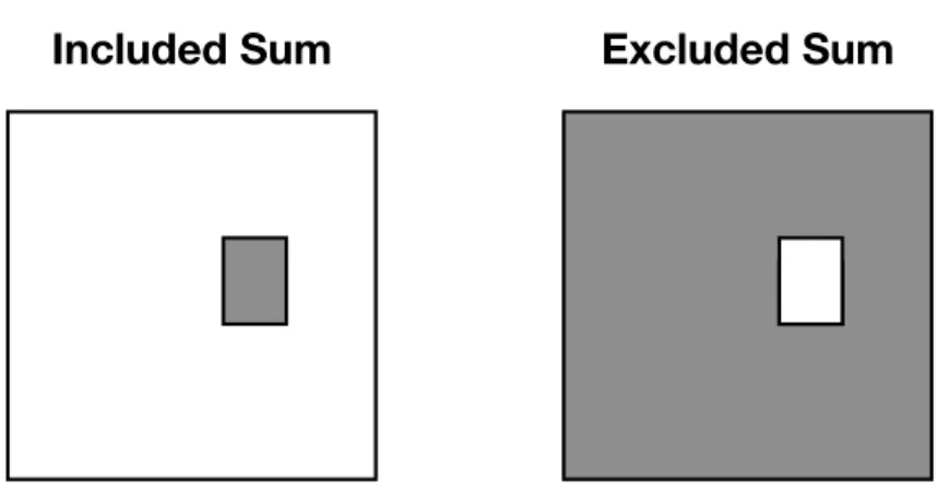
At a high level, the included and excluded sums problems require computing reductions over many different (but possibly overlapping) regions in a matrix (one corresponding to each entry in the matrix). The problems take as input a matrix and a “box size” (or side lengths defining a rectangular region, or “box”). Given a box size, each location in the matrix defines a spatial box of that size. An algorithm for included sums outputs another matrix of the same size as the input matrix where each entry is the reduction of all elements contained in the box for that entry. The “excluded sums problem” is the inverse of the included sums problem: each entry in the output matrix is the reduction of all elements outside of the corresponding box. As we will see, a solution for included sums does not directly translate into a solution for excluded sums for general operators.
X
Included Sum
Excluded Sum
Figure 1-1: An example of the included and excluded sums in two dimensions for one box. The grey represents the region of interest to be reduced. Typically, the included and excluded sums problem require computing the reduction for all such regions (only one is depicted in the figure for illustration).
or excluded region for all points in the matrix. If we were only interested in one box (or one excluded region) a single pass over the matrix would suffice. If there are 𝑁 points in the matrix and the box size is 𝑅, naively summing elements in each box for the included sum takes 𝑂(𝑁𝑅) work (𝑂(𝑁(𝑁 − 𝑅)) for the naive excluded sum) and involves many repeated computations. An example of one entry of the included and excluded sum can be found in Figure 1-1.
The included and excluded sums problems appear in a variety of multidimensional compu-tations. For example, the integral image problem (or summed-area table) [8,12] pre-processes an image to answer queries for the sum of elements in arbitrary rectangular subregions of a matrix in constant time. The integral image has applications in real-time image processing and filtering [19]. The fast multipole method (FMM) is a widely-used numerical approxima-tion for the calculaapproxima-tion of long-ranged forces in various 𝑁-particle simulaapproxima-tions [3, 17]. The essence of the FMM is a reduction of a neighoring subregion’s particles, excluding particles too close, to a multipole to allow for fewer pairwise calculations [9,13].
Summation Without Inverse
An obvious solution to first solve the included sums problem and subtract out the results from reducing the entire tensor fails for functions of interest which might represent singularities (e.g. in physics 𝑁-particle simulations) [14] or for operators without inverse (such as max). Even for functions with an inverse, subtracting floating-point values suffers from catastrophic
cancellation [14, 38]. Therefore, we require algorithms without subtraction for the excluded sums problem.
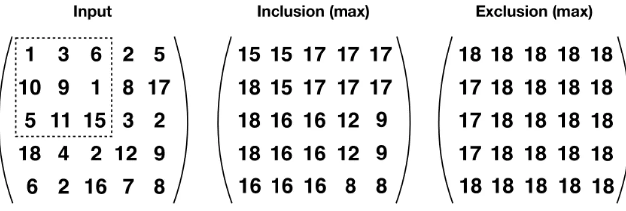
More generally, algorithms for the included and excluded sums problem should apply to any associative operator (with or without an inverse). In Figure 1-2, we present an example of the included and excluded sums problem with the max operator (which does not have an inverse).
Input Inclusion (max) Exclusion (max)
1
3
6 2 5
10 9
1 8 17
5
15 3 2
4
2
9
6 2
7 8
18
11
12
16
15
18
18
16
9
9
8 8
18
16
12
16
16
15
15
16
16
17 17 17
17 17 17
12
16
18
17
17
18
17
18
18
18
18
18
18
18
18
18 18 18
18 18 18
18
18
18
18
18
18
Figure 1-2: An example of the included and excluded sums problems in two dimensions with a box size of 3 × 3 and the max operator. The dotted box represents an example of a 3 × 3 box in the matrix, but the included and excluded sums problem computes the inclusion or exclusion regions for all 3 × 3 boxes.Corners Algorithm for Excluded Sums
Since naive algorithms for reducing regions of a tensor may waste work by recomputing reductions for overlapping regions, researchers have proposed algorithms that reuse the work of reducing regions of a tensor. Demaine et al. [14] introduced an algorithm to compute the excluded sums in arbitrary dimensions without subtraction, which we will call the corners algorithm. To our knowledge, the corners algorithm is the fastest algorithm for the excluded sums problem.
Given a 𝑑-dimensional tensor and a length 𝑑 vector of box side lengths, the corners algorithm computes the excluded sum for all (𝑁) boxes of that size. At a high level, the corners algorithm decomposes the excluded region for each box into 2𝑑 disjoint regions (one
corresponding to each corner of that box, or to each vertex in 𝑑-dimensions) such that summing all of the points in the 2𝑑 regions exactly matches the excluded region. The
each of the disjoint regions.
The original article that proposed the corners algorithm does not include a formal analysis of its runtime or space usage in arbitrary dimensions. Given a 𝑑-dimensional tensor of 𝑁 points, the corners algorithm takes Ω(2𝑑𝑁 ) work to compute the excluded sum in the best
case because there are 2𝑑 corners and each one requires Ω(𝑁) work to account for the
contribution to each excluded box. The bound is tight: given arbitrary extra space, the corners algorithm takes 𝑂(2𝑑𝑁 ) work. An in-place (uses space sublinear in the input size)
corners algorithm takes 𝑂(2𝑑𝑑𝑁 ) work.
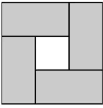
Figure 1-3: An example of the corners algorithm for one box in two dimensions. The grey regions represent excluded regions computed via prefix and suffix sums.
To our knowledge, the best lower bound for the work and space usage for any algorithm for excluded sums is Ω(𝑁) because any algorithm has to read in the entire input tensor (of size 𝑁) at least once and output a tensor of size Ω(𝑁).
Prefix and Suffix Sums
As we will formalize in Chapter 3, an efficient implementation of either the corners algorithm or the DRES algorithm requires a fast prefix and suffix sum implementation since prefix and suffix sums are core subroutines in both algorithms. For simplicity, we will discuss prefix sums for the rest of this thesis, but all of the techniques that we explore for prefix sums also apply to suffix sums.
The prefix sum (also known as scan) [5] operation is one of the most fundamental building blocks of parallel algorithms. Prefix sums are so ubiquitous that they have been included as primitives in some languages such as C++ [11], and more recently have been considered
as a primitive for GPU computations in CUDA [18]. Furthermore, parallel prefix sums (or analogously, a pairwise summation) achieve high numerical accuracy on finite-precision floating-point numbers [21] compared to a naive sequential reduction [20]. Therefore, parallel prefix sums are well-suited to scientific computing applications such as the FMM which optimize for both performance and accuracy.
(a) Performance (b) Accuracy
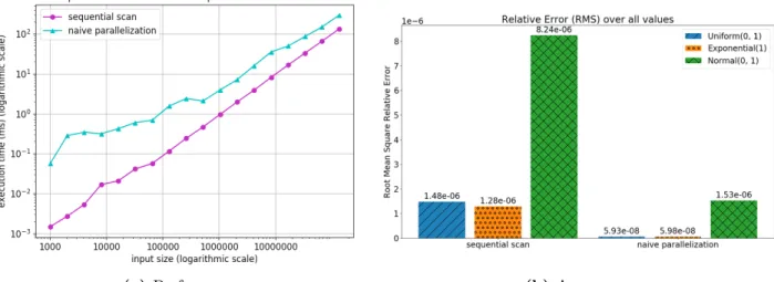
Figure 1-4: Performance and accuracy of the naive sequential prefix sum algorithm compared to an unoptimized parallel version on a 40-core machine. Clearly, there is no speedup for the parallel version, and in fact, it makes it even slower. For the accuracy comparison, we define the error as the root mean square relative error over all outputs of the prefix sum array compared to a higher precision reference at the equivalent index. The input is an array of 215 single-precision floating point numbers, according to a distribution in the legend. The options are random numbers either drawn from Unif(0, 1), Exp(1), or Normal(0, 1). On these inputs, the parallel version is on average around 17× more accurate.
Although the canonical parallel prefix sum should be faster in theory, traditional im-plementations on general-purpose multicores exhibit several performance issues. As shown in Figure 1-4, an unoptimized parallel prefix sum is slower than the simplest serial algorithm. The parallel prefix sum is recursive, which generates function call overhead. The parallel prefix sum is work-efficient but has a constant factor of extra work when compared to the serial version [5]. Furthermore, there is additional overhead in parallelization due to schedul-ing [27]. Parallel implementations without careful coarsenschedul-ing may also run into cache-line conflicts and contention [15,36]. The serial algorithm takes advantage of prefetching [34] be-cause it just requires a straightforward pass through the input, while the parallel algorithm accesses elements out of order in a tree-like traversal [5]. Finally, as we will see in Chapter 4,
the traditional parallel algorithm does not take advantage of data-level parallelism via vec-torization. An efficient implementation of parallel prefix sum requires careful parallelization and optimization to take advantage of task-level and data-level parallelism effectively.
The highlights of our results for prefix sum can be summarized by Figure 1-5, which shows the trade-offs between performance and accuracy for various prefix sum algorithms at three input sizes - 215, 222, and 227. These input sizes highlight the trends - for smaller inputs, the
serial algorithms perform better, and for larger inputs, PBBSLIB and block_hybrid_reduce both have similar performance due to reaching the maximum memory bandwidth. The differences are most pronounced for our algorithms in the middle-sized plot. The full plots in Chapter 4 have the details. The top right corner of each matrix represents algorithms that are highly performant and accurate. Our algorithms are sequential intrinsics (single-threaded), block_hybrid, and block_hybrid_reduce.
Figure 1-5: Three highlight matrices of the trade-offs between performance and accuracy. The input size is either 215 (left), 222 (center), or 227 (right) floats, and tests are run on a 40-core machine. Accuracy is measured as 1
RMSE and plotted on a logarithmic scale, where RMSE is defined in Section 4.3, for the random numbers uniformly distributed between 0 and 1. Performance (or observed parallelism) is measured as 𝑇1
𝑇40ℎ, where 𝑇40ℎ is the parallel time on the Supercloud 40-core Machine with 2-way hyper-threading, and 𝑇1 is the serial time of the naive sequential prefix sum on the same machine.
Contributions
Our contributions can be divided into two main categories: results for included and excluded sums, and results for prefix sums.
Our main contribution for excluded sums is the dimension-reduction excluded-sums (DRES) algorithm, an asymptotically improved algorithm for the excluded sums problem in arbitrary dimensions. Along the way, we present an efficient algorithm for included sums called the INCSUM algorithm. We measure multithreaded algorithms in terms of their work and span, or longest chain of sequential dependencies [10, Chapter 27]. Chapter 2 formalizes the dynamic multithreading model.
The DRES and INCSUM algorithms take as input the following parameters: • a 𝑑-dimensional tensor 𝒜 with 𝑁 entries,
• the size of the excluded region (the “box size”), and • a binary associative operator ⊕.
Both algorithms output another 𝑑-dimensional tensor ℬ with 𝑁 entries where each entry is the excluded or included sum (respectively) corresponding to that point in the tensor under the operator ⊕.
Our contributions towards excluded and included sums are as follows:
• The dimension-reduction excluded-sums (DRES) algorithm, an asymptotically im-proved algorithm for the excluded sums problem in arbitrary dimensions.
• Theorems showing that DRES computes the excluded sum in 𝑂(𝑑𝑁) work and in 𝑂 (︂ 𝑑2∑︀𝑑 𝑖=1 lg 𝑛𝑖 )︂
span for a 𝑑-dimensional tensor with 𝑁 points where each dimension 𝑖 = 1, . . . , 𝑑 has length 𝑛𝑖.
• An implementation of DRES in C++ for an experimental evaluation on the horizon. Our results for prefix sums are as follows:
• The block-hybrid (BH) algorithm for prefix sums, a data-parallel and task-parallel algorithm for prefix sums, and a less accurate, faster variant.
• A proof of the observation that reducing the span of a prefix sum algorithm improves both its parallelism and worst case error bound in floating point arithmetic.
• An implementation of the block-hybrid algorithm in C++ / Cilk [7].
• An experimental comparison of prefix sum algorithms that shows that the BH algo-rithm is up to 2.5× faster on inputs that fit in cache and 8.4× more accurate than state-of-the-art CPU parallel prefix sum algorithms. We also present a variation of BH that is faster on larger inputs and 2.6× more accurate compared to the same benchmarks, in addition to being up to 2.5× faster on inputs that fit in cache.
• An evaluation of prefix sums on a CPU versus a GPU that shows the BH algorithm variant on a CPU is at least 1.5× more cost-efficient than the state-of-the-art GPU implementation (using AWS pricing [2]).
Map
The rest of this thesis is organized as follows. In Chapter 2, we review background on prefix sums, cost models for algorithm analysis in the remainder of the thesis, and our experimental setup. We present and analyze algorithms for excluded and included sums in Chapter 3. We introduce the block-hybrid algorithm and two variants for prefix sums, and conduct an experimental study of prefix sum algorithms in Chapter 4. Finally, we provide closing remarks in Chapter 5.
Chapter 2
Preliminaries
This section reviews the prefix sum primitive as well as models for dynamic multithreading and numerical accuracy that we will use to analyze algorithms in this thesis. The included sums, excluded sums, and prefix sums software are implemented in Cilk [7, 24], which is a linguistic extension to C++ [33]. Therefore, we describe Cilk-like pseudocode and use the model of multithreading underlying Cilk, although the pseudocode can be applied to any arbitrary fork-join parallelism model.
Prefix and Suffix Sums
We first review the all-prefix-sums operation [5] (or scan) as a primitive operation that we will use throughout this thesis (note that this is an inclusive scan).
Definition 1 (All-prefix-sums Operation) The all-prefix-sums operation takes a binary associative operator ⊕ (for example, addition, multiplication, minimum or maximum), and
an ordered set of 𝑛 elements
[𝑎0, 𝑎1, . . . , 𝑎𝑛−1]
and returns the ordered set
Example. If ⊕ is addition, then the all-prefix-sums operation on the ordered set
[3 1 7 0 4 1 6 3]
would return
[3 4 11 11 15 16 22 25].
The suffix sum is the reverse of the prefix sum:
Definition 2 (All-suffix-sums Operation) The all-suffix-sums operation takes a binary associative operator ⊕ (for example, addition, multiplication, minimum or maximum), and
an ordered set of 𝑛 elements
[𝑎0, 𝑎1, . . . , 𝑎𝑛−1]
and returns the ordered set
[(𝑎0⊕ 𝑎1⊕ . . . ⊕ 𝑎𝑛−1), (𝑎1⊕ . . . ⊕ 𝑎𝑛−1), . . . , 𝑎𝑛−1].
Additionally, Reduce, which we will see in Chapter 4, takes the same arguments as prefix sum, but only returns the single element 𝑎0⊕ 𝑎1⊕ . . . ⊕ 𝑎𝑛−1 (the last element).
Analysis of Multithreaded Algorithms
The linguistic model for multithreaded pseudocode from [10, Chapter 27] follows MIT Cilk [24]. It augments serial code with three keywords: spawn, sync, and parallel; the last of which can be implemented with the first two.
The spawn keyword before a function call creates nested parallelism. The parent func-tion executes a spawn and can execute in parallel with the spawned child subroutine. There-fore, the code that immediately follows the spawn may execute in parallel with the child, rather than waiting for it to complete as in a serial function call. A parent function cannot safely use the values returned by its children until after a sync statement, which causes the function to wait until all of its spawned children to complete before proceeding to the code after the sync. Every function also implicitly syncs before it returns, preventing orphaning.
The spawn and sync keywords denote logical parallelism in a computation, but do not require parts of a computation to run in parallel. At runtime, a scheduler determines which subroutines run concurrently by assigning them to different cores in a multicore machine. Cilk has a runtime system that implements a provably efficient work-stealing scheduler [7].
Parallel loops can be expressed by preceding an ordinary for with the keyword parallel, which indicates that all iterations of the loop may run in parallel. Parallel loops can be implemented by parallel divide-and-conquer recursion using spawn and sync.
We use the dynamic multithreading model to measure the asymptotic costs of multi-threaded algorithms in terms of their work and span [10, Chapter 27]. The work is the total time to execute the entire algorithm one one processor. The span1 is the longest serial chain
of dependencies in the computation (or the runtime in instructions on an infinite number of processors). For example, a parallel for loop over 𝑁 iterations of 𝑂(1) work per iteration has 𝑂(log 𝑁) span2 in the dynamic multithreading model.
Accuracy Model
Sums of floating point numbers in scientific computing are ubiquitous and require careful consideration of the accumulation of roundoff errors. Because floating-point addition is non-associative on computers, standard compilers such as Clang and GCC are not allowed to reorder operations in the summation of an arbitrary sequence of floating point operations without breaking IEEE or ISO guarantees (this restriction can be lifted with certain compiler flags, but the results are no longer guaranteed). The effect would be different summation results with different degrees of error, when dissimilar sized numbers are added together. There has been plenty of research carried out on numerical stability, most notably by Higham [21] [20]. As we find out analytically and experimentally, the order in which we sum an arbitrary sequence of floating point numbers has a great effect on the accuracy of a result, depending on the input values. Moreover, if we can understand how to best mitigate floating point roundoff error and achieve high accuracy in our summations, we can utilize this skill set in designing serial and parallel algorithms that achieve good compromises of performance and accuracy.
1Sometimes called critical-path length or computational depth. 2In this thesis, log is always base 2.
We use a standard accuracy model for floating point arithmetic, as described by Higham [20] and Goldberg [16].
𝑓 𝑙(𝑥 op 𝑦) = (𝑥 op 𝑦)(1 + 𝛿), |𝛿| ≤ 𝑢, op = +, −, *, / (2.1)
where 𝛿 is a small error associated with the floating point representation of the calculation after correct rounding, and 𝑢 is the unit roundoff (or machine precision), which, for single precision floating points, is 5.96×10⁻⁸, and for doubles is 1.11×10⁻¹⁶. We are also assuming
the use of a guard digit, which is standard. For more details on floating point arithmetic, see [16] and the rest of [20]. We use the following summarized results from Higham’s work on the accuracy of floating point summation to guide our accuracy analysis and evaluation:
Worst Case Error Bounds. In summation, we are evaluating an expression of the form 𝑆𝑛 =
∑︀𝑛−1
𝑖=0 𝑥𝑖, where 𝑥0, ..., 𝑥𝑛−1 are real numbers. As we will elucidate in Chapter 4,
Higham [20] shows that the worst case error bound for summing an array of numbers in the naive way (a running total from left to right) has an error constant of 𝑂(𝑛), i.e., the length of the longest chain of additions. Further, a pairwise summation, which we will describe in Chapter 4 and analogize to a parallel-prefix computation, has a worst case error bound constant of 𝑂(log 𝑛). We will apply these error bounds to our prefix sum algorithms. Higham notes that when 𝑛 is very large, pairwise summation is an efficient compromise between performance and accuracy.
Experimental Analysis and Results. Rounding error bounds tend to be very pessimistic, since they are worst case bounds. Higham mentions that it is also important to experimen-tally evaluate the accuracy of summations. We use several ideas from his methodologies: using higher precision numbers as a reference point, using random numbers from uniform, exponential and normal distributions as input, and the Kahan summation algorithm as a benchmark [16]. Further, we use his results on statistical estimates of accuracy on pairwise summation to affirm its performance. Our decision to use root mean square relative error to compare the results is also inspired by his discussion.
Experimental Setup
This section summarizes the shared-memory multicore machines, compilers, and software used for all experimental evaluation in this thesis. The following are the references names that will be used throughout.
AWS 18-core Machine (c4.8xlarge) An 18-core machine with 2 × Intel Xeon CPU E5-2666 v3 (Haswell) @ 2.90GHz processors, each with 9 cores per processor, with 2-way hyperthreading. Each processor has a 1600MHz bus and a 25MB L3 cache. Each core has a 256KB L2 cache, a 32KB L1 data cache, and a 32KB L1 instruction cache. The cache line size is 64B. There is a total of 60GB DRAM on the machine. The theoretical maximum memory bandwidth is 51.2 GB/second. The cores have AVX2 (and earlier AVX, SSE) instruction set extensions.
Supercloud 40-core Machine A 40-core machine with 2 × Intel Xeon Gold 6248 @ 2.50GHz processors, each with 20 cores per processor, with 2-way hyperthreading. Each processor has a 2993MHz bus and a 27.5MB L3 cache. Each core has a 1MB L2 cache, a 32KB L1 data cache, and a 32KB L1 instruction cache. The cache line size is 64B. There is a total of 384GB DRAM on the machine. The theoretical maximum memory bandwidth is 93.4GB/second. The cores have AVX512 (and earlier AVX2, AVX, SSE) instruction set extensions.
Affordable AWS Machine (c5.xlarge) A 2-core machine with 1 × Intel Xeon Platinum 8124M CPU @ 3.00GHz processors, each with 2 cores per processor, with 2-way hyperthread-ing. The processor has a 25MB L3 cache. Each core has a 1MB L2 cache, a 32KB L1 data cache, and a 32KB L1 instruction cache. The cache line size is 64B. There is a total of 8GB DRAM on the machine. The cores have AVX512 (and earlier AVX2, AVX, SSE) instruction set extensions.
Volta GPU The Supercloud 40-core machine also has 2 NVIDIA Volta V100 GPUs at-tached. The GPU has 32GB RAM. When run with just 1 GPU, we note that this is the same as the p3.2xlarge Amazon EC2 instance [1], and use this for pricing comparisons against the Affordable AWS Machine.
Compiler As stated earlier, all the code is implemented in C++ using Cilk for fork-join parallelism. The compiler used is an extended version of Clang version 8, called Tapir/LLVM
[28]. The -O3 and -march=native compiler flags are used throughout the experiments for maximum performance.
Boost The Boost C++ Library is used to carry out the accuracy experiments regarding floating point summation. In particular, Boost multi-precision floating point numbers [26] are used, providing 100 decimal digits of precision. The experiments can then calculate summation results much closer to the true real value, and is the basis for which we compare relative error against for the different methods of summation. Higham [20] uses a similar technique of comparing to a higher precision reference point.
Code The code will be available at https://github.com/seanfraser/thesis at the time of publication. Expected by the end of May 2020.
Chapter 3
Included and Excluded Sums
Outline. In this chapter, we present algorithms for included and excluded sums in arbitrary dimensions. We begin with necessary preliminaries for indexing and defining ranges in tensors to understand the later algorithms. We conclude with two potential applications for included and excluded sums, and their relation to prefix sums.
3.1
Tensor Preliminaries
We discuss order-𝑑 tensors in a particular orthogonal basis. That is, tensors are 𝑑-dimensional arrays of elements over some field ℱ, usually the real or complex numbers. We denote tensors by capital script letters 𝒜 and vectors by lowercase boldface letters a.
Definition 3 (Index domain) An index domain 𝑈 is the cross product 𝑈 = 𝑈1× 𝑈2×
. . . × 𝑈𝑑 where 𝑑 ≥ 1 and for 𝑖 = 1, 2, . . . , 𝑑, we have 𝑈𝑖 = {0, 1, . . . , 𝑛𝑖 − 1} where 𝑛𝑖 ≥ 1.
That is, dimensions are 1-indexed and coordinates start at 0.
A tensor 𝒜 is a mapping such that 𝒜 : 𝑈 → F for some index domain 𝑈 and for some field F. The length of dimension 𝑖 of tensor 𝒜 is 𝑛𝑖.
We can denote a particular element of an index domain as an index x = (𝑥1, 𝑥2, . . . , 𝑥𝑑)
where for all 𝑖 = 1, 2, . . . , 𝑑, 0 ≤ 𝑥𝑖 ≤ 𝑛𝑖 − 1. Sometimes for simplicity of notation, we will
We use 𝑥 : 𝑥′ to denote a range of indices along a particular dimension and : without
bounds to indicate all elements along a particular dimension. For example, the middle 𝑛/2 columns of an 𝑛 × 𝑛 matrix 𝒜 would be written 𝒜(:, 𝑛/4 : 3𝑛/4). A range of indices defines a subtensor. A tensor defines a value at each index (i.e. 𝒜[x] ∈ F). The value of a tensor at a range of indices is the sum (or reduction) of the values of the tensor at each index in the range.
Next, we introduce box notation, which we will use to formally define the included and excluded sums problems.
Definition 4 (Box) A box of an index domain 𝑈 cornered at x = (𝑥1, . . . , 𝑥𝑑) ∈ 𝑈, x′ =
(𝑥′1, . . . , 𝑥′𝑑) ∈ 𝑈 which is denoted 𝐵 = (𝑥1 : 𝑥′1, 𝑥2 : 𝑥′2, . . . , 𝑥𝑑 : 𝑥′𝑑) ⊆ 𝑈 is the region
{𝑦 = (𝑦1, 𝑦2, . . . , 𝑦𝑑) ⊆ 𝑈 : 𝑥1 ≤ 𝑦1 < 𝑥′1, 𝑥2 ≤ 𝑦2 < 𝑥′2, . . . , 𝑥𝑑 ≤ 𝑦𝑑 < 𝑥′𝑑}. For all
𝑖 = 1, 2, . . . , 𝑑, 𝑥𝑖 < 𝑥′𝑖.
Definition 5 (Box-side lengths) Given an index domain 𝑈 and a box 𝐵 = (𝑥1 : 𝑥′1, 𝑥2 :
𝑥′2, . . . , 𝑥𝑑 : 𝑥′𝑑) ⊆ 𝑈 , the box-side lengths are denoted ℓ𝐵 = (𝑥′1− 𝑥1, 𝑥′2− 𝑥2, . . . , 𝑥′𝑑− 𝑥𝑑),
or the length of the box in each dimension.
3.2
Problem Definitions
In this section we describe the included and excluded sums problems. Throughout this section, let 𝒜 : 𝑈 → F be a 𝑑-dimensional tensor and k = (𝑘1, . . . , 𝑘𝑑) be a vector of
box-side lengths. For simplicity in the pseudocode, we will assume 𝑛𝑖 mod 𝑘𝑖 = 0 for all
𝑖 = 1, 2, . . . , 𝑑. In implementations, the input can either be padded with the identity to make this true, or add in extra code to deal with unaligned boxes.
Problem 1 (Included Sums Problem) An algorithm for the included sums problem
takes as input a tensor 𝒜 and vector of box-side lengths k. It outputs a new tensor ℬ : 𝑈 → F such that every index x = (𝑥1, . . . , 𝑥𝑑) of ℬ maps to the sum of elements at all indices inside
For example, the included sums problem in one dimension is the problem of finding the sum of each run of length 𝑘 in an array of length 𝑛. In two dimensions, the included sums problem is finding the sum of all elements in every 𝑘1× 𝑘2 box in an 𝑛1× 𝑛2 matrix.
The excluded sums problem definition is the inverse of the included sums: every index in the output tensor ℬ maps to the sum of element at all indices outside of the box cornered at that index.
3.3
INCSUM Algorithm
First, we will present a linear-time algorithm INCSUM to solve the included sums problem in one dimension and demonstrate how to extend it to arbitrary dimensions.
Included Sums in One Dimension
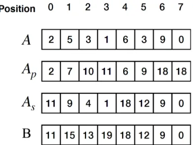
Let 𝒜 be a list of length 𝑁 and 𝑘 be the (scalar) length of the box. For simplicity, assume 𝑁 mod 𝑘 = 0(we can pad the list length). At a high level, the incsum_1D algorithm generates two intermediate lists 𝐴𝑝, 𝐴𝑠 of length 𝑁 each and does 𝑁/𝑘 prefix and suffix sums of length
𝑘 each, respectively. By construction, for 𝑥 = 0, 1, . . . , 𝑁 − 1, 𝒜𝑠[𝑥] = 𝒜[︀𝑥 : ⌈︀𝑥+1𝑘 ⌉︀ · 𝑘]︀ and
𝒜𝑝[𝑥] = 𝒜
[︀⌊︀𝑥
𝑘⌋︀ · 𝑘 : 𝑥 + 1]︀.
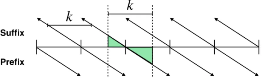
We begin with pseudocode for the included sum in one dimension in Figure 3-1. We then illustrate the ranged prefix and suffix sums in Figure 3-2 and present a worked example in Figure 3-3.
The algorithm in Figure 3-1 is clearly linear in the number of elements in the list since the total number of loop iterations is 2𝑁. As mentioned in the introduction, a naive algorithm for included sums takes 𝑂(𝑁𝑘) where 𝑁 is the number of elements and 𝑘 is the box length.
We will now show that incsum_1D computes the included sum.
Lemma 1 incsum_1D solves the included sums problem in one dimension.
Proof. Consider a one-dimensional list 𝒜 with 𝑁 elements and box length 𝑘. We will show that for each 𝑥 = 0, 1, . . . , 𝑁 − 1, ℬ(𝑥) contains the desired sum. For 𝑥 mod 𝑘 = 0, this holds by construction. For all other 𝑥, the previously defined prefix and suffix sum give
incsum_1D(𝐴, 𝑁, 𝑘)
1 ◁ Input: list 𝐴 of size 𝑁, included sum length 𝑘
2 ◁ Output: list 𝐵 of size 𝑁 where each entry 𝐵[𝑖] = 𝐴[𝑖 : 𝑖 + 𝑘] for 𝑖 = 0, 1, . . . 𝑁 − 1. 3 𝐵[𝑁]
4 𝐴𝑝 ← 𝐴, 𝐴𝑠← 𝐴
5 ◁ 𝑘-wise prefix sum along row 6 parallel for i ← 0 to N /k − 1 7 for j ← 1 to 𝑘 − 1 8 𝐴𝑝[i (𝑁/𝑘) + 𝑗]+ =𝐴𝑝[i (𝑁/𝑘) + 𝑗 − 1] 9 for j ← 𝑘 − 2 downto 0 10 𝐴𝑠[i (𝑁/𝑘) + 𝑗]+ =𝐴𝑠[i (𝑁/𝑘) + 𝑗 + 1] 11 parallel for i ← 0 to N − 1 12 if i mod 𝑘==0 13 𝐵[i ] = 𝐴𝑠[i ] 14 else 15 𝐵[i ] = 𝐴𝑠[i ] + 𝐴𝑝[i + k − 1] 16 return 𝐵
Figure 3-1: Pseudocode for the included sum in one dimension.
k
Suffix
Prefix
k
Figure 3-2: Computing the included sum in one dimension in linear time.
the desired result. Recall that ℬ[𝑥] = 𝒜𝑝[𝑥 + 𝑘 − 1] + 𝒜𝑠[𝑥], 𝒜𝑠[𝑥] = 𝒜[𝑥 :
⌈︀𝑥+1
𝑘 ⌉︀ · 𝑘], and
𝒜𝑝[𝑥 + 𝑘 − 1] = 𝒜[⌊𝑥+𝑘−1𝑘 ⌋ · 𝑘 : 𝑥 + 𝑘]. Also note that ⌊𝑥+𝑘−1𝑘 ⌋ = ⌈𝑥+1𝑘 ⌉ for all 𝑥 mod 𝑘 ̸= 0.
Therefore, ℬ[𝑥] = 𝒜𝑝[𝑥 + 𝑘 − 1] + 𝒜𝑠[𝑥] = 𝒜 [︂ 𝑥 :⌈︂ 𝑥 + 1 𝑘 ⌉︂ · 𝑘 ]︂ + 𝒜[︂⌊︂ 𝑥 + 𝑘 − 1 𝑘 ⌋︂ · 𝑘 : 𝑥 + 𝑘 ]︂ = 𝒜[𝑥 : 𝑥 + 𝑘]
Figure 3-3: Example of computing the included sum in one dimension with 𝑁 = 8, 𝑘 = 4.
Generalizing to Arbitrary Dimensions
Next, we demonstrate how to extend the one-dimensional INCSUM algorithm to solve the included sums problem for a 𝑑-dimensional tensor of 𝑁 points in 𝑂(𝑑𝑁) work.
At a high level, we apply the same one-dimensional INCSUM algorithm along every row of each dimension. For example, Figure 3-4 shows how to use the result of the included sum along one dimension of a matrix to find the included sum of a two-dimensional box.
f f
INCSUM in first dimension INCSUM in second dimension on result
Subroutines incsum_prefix_along_row and incsum_suffix_along_row in Fig-ures 3-5 and 3-6 (respectively) compute the ranged prefix and suffix sum that later combine to form the included sum along an arbitrary row of the tensor in higher dimensions.
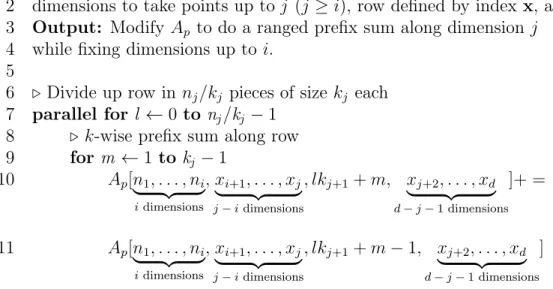
incsum_prefix_along_row(𝐴𝑝, i , j , x = (𝑥1, . . . , 𝑥𝑑), k = (𝑘1, . . . , 𝑘𝑑))
1 Input: Tensor 𝐴𝑝 (𝑑 dimensions, side lengths (𝑛1, . . . , 𝑛𝑑)), dimensions reduced up to i,
2 dimensions to take points up to j (𝑗 ≥ 𝑖), row defined by index x, and box-lengths k. 3 Output: Modify 𝐴𝑝 to do a ranged prefix sum along dimension 𝑗
4 while fixing dimensions up to 𝑖. 5
6 ◁ Divide up row in 𝑛𝑗/𝑘𝑗 pieces of size 𝑘𝑗 each
7 parallel for l ← 0 to nj/kj − 1
8 ◁ 𝑘-wise prefix sum along row
9 for m ← 1 to kj − 1 10 𝐴𝑝[𝑛1, . . . , 𝑛𝑖 ⏟ ⏞ 𝑖 dimensions , 𝑥𝑖+1, . . . , 𝑥𝑗 ⏟ ⏞ 𝑗 − 𝑖 dimensions , 𝑙𝑘𝑗+1+ 𝑚, 𝑥𝑗+2, . . . , 𝑥𝑑 ⏟ ⏞ 𝑑 − 𝑗 − 1 dimensions ]+ = 11 𝐴𝑝[𝑛1, . . . , 𝑛𝑖 ⏟ ⏞ 𝑖 dimensions , 𝑥𝑖+1, . . . , 𝑥𝑗 ⏟ ⏞ 𝑗 − 𝑖 dimensions , 𝑙𝑘𝑗+1+ 𝑚 − 1, 𝑥𝑗+2, . . . , 𝑥𝑑 ⏟ ⏞ 𝑑 − 𝑗 − 1 dimensions ]
Figure 3-5: Ranged prefix along row.
incsum_suffix_along_row(𝐴𝑠, i , j , x = (𝑥1, . . . , 𝑥𝑑), k = (𝑘1, . . . , 𝑘𝑑))
1 Input: Tensor 𝐴𝑠 (𝑑 dimensions, side lengths (𝑛1, . . . , 𝑛𝑑)), dimensions reduced up to i,
2 dimensions to take points up to j (𝑗 ≥ 𝑖), row defined by index x, and box-lengths k. 3 Output: Modify 𝐴𝑠 to do a ranged suffix sum along dimension 𝑗
4 while fixing dimensions up to 𝑖. 5
6 ◁ Divide up row in 𝑛𝑗/𝑘𝑗 pieces of size 𝑘𝑗 each
7 parallel for l ← 0 to nj/kj − 1
8 ◁ 𝑘-wise suffix sum along row
9 for m ← 𝑘𝑗 − 2 downto 0 10 𝐴𝑠[𝑛1, . . . , 𝑛𝑖 ⏟ ⏞ 𝑖 dimensions , 𝑥𝑖+1, . . . , 𝑥𝑗 ⏟ ⏞ 𝑗 − 𝑖 dimensions , 𝑙𝑘𝑗+1+ 𝑚, 𝑥𝑗+2, . . . , 𝑥𝑑 ⏟ ⏞ 𝑑 − 𝑗 − 1 dimensions ]+ = 11 𝐴𝑠[𝑛1, . . . , 𝑛𝑖 ⏟ ⏞ 𝑖 dimensions , 𝑥𝑖+1, . . . , 𝑥𝑗 ⏟ ⏞ 𝑗 − 𝑖 dimensions , 𝑙𝑘𝑗+1+ 𝑚 + 1, 𝑥𝑗+2, . . . , 𝑥𝑑 ⏟ ⏞ 𝑑 − 𝑗 − 1 dimensions ]
Figure 3-6: Ranged suffix along row.
and suffix sums along an arbitrary dimension to compute the included sum in a row of the tensor.
incsum_result_along_row(A, i , j , x = (𝑥1, . . . , 𝑥𝑑), k = (𝑘1, . . . , 𝑘𝑑), 𝐴𝑝, 𝐴𝑠)
1 Input: Tensor 𝐴 (𝑑 dimensions, side lengths (𝑛1, . . . , 𝑛𝑑)) to write the output,
2 dimensions reduced up to i, dimensions to take points up to j (𝑗 ≥ 𝑖),
3 row defined by index x, box-lengths k, ranged prefix and suffix tensors 𝐴𝑝, 𝐴𝑠.
4 Output: Modify 𝐴 with the included sum along the specified row in dimension 𝑗. 5
6 parallel for ℓ ← 1 to nj
7 ◁ If on a boundary, just assign to the beginning of the k-wise suffix 8 ◁ (equal to the sum of k elements in this window)
9 if ℓ mod 𝑘𝑗 == 0 10 𝐴[𝑛1, . . . , 𝑛𝑖 ⏟ ⏞ 𝑖 dimensions , 𝑥𝑖+1, . . . , 𝑥𝑗 ⏟ ⏞ 𝑗 − 𝑖 dimensions , ℓ, 𝑥𝑗+2, . . . , 𝑥𝑑 ⏟ ⏞ 𝑑 − 𝑗 − 1 dimensions ]= 11 𝐴𝑠[𝑛1, . . . , 𝑛𝑖 ⏟ ⏞ 𝑖 dimensions , 𝑥𝑖+1, . . . , 𝑥𝑗 ⏟ ⏞ 𝑗 − 𝑖 dimensions , ℓ, 𝑥𝑗+2, . . . , 𝑥𝑑 ⏟ ⏞ 𝑑 − 𝑗 − 1 dimensions ] 12 else
13 ◁Otherwise, add in relevant prefix and suffix 14 𝐴[𝑛1, . . . , 𝑛𝑖 ⏟ ⏞ 𝑖 dimensions , 𝑥𝑖+1, . . . , 𝑥𝑗 ⏟ ⏞ 𝑗 − 𝑖 dimensions , ℓ, 𝑥𝑗+2, . . . , 𝑥𝑑 ⏟ ⏞ 𝑑 − 𝑗 − 1 dimensions ]= 15 𝐴𝑠[𝑛1, . . . , 𝑛𝑖 ⏟ ⏞ 𝑖 dimensions , 𝑥𝑖+1, . . . , 𝑥𝑗 ⏟ ⏞ 𝑗 − 𝑖 dimensions , ℓ, 𝑥𝑗+2, . . . , 𝑥𝑑 ⏟ ⏞ 𝑑 − 𝑗 − 1 dimensions ] 16 +𝐴𝑝[𝑛1, . . . , 𝑛𝑖 ⏟ ⏞ 𝑖 dimensions , 𝑥𝑖+1, . . . , 𝑥𝑗 ⏟ ⏞ 𝑗 − 𝑖 dimensions , ℓ + 𝑘𝑗+1− 1, 𝑥𝑗+2, . . . , 𝑥𝑑 ⏟ ⏞ 𝑑 − 𝑗 − 1 dimensions ]
Figure 3-7: Computes the included sum along a given row.
The function incsum_along_dim in Figure 3-8 computes the included sum for a specific dimension of the tensor along all rows. Finally, incsum in Figure 3-9 computes the full included sum along all dimensions.
incsum_along_dim(A, i , j , k = (𝑘1, . . . , 𝑘𝑑))
1 Input: Tensor 𝐴 (𝑑 dimensions, side lengths (𝑛1, . . . , 𝑛𝑑)) to write the output,
2 dimensions reduced up to i, dimensions to take points up to j (𝑗 ≥ 𝑖), 3 row defined by index x, box-lengths k.
4 Output: Modify 𝐴 with the included sum in dimension 𝑗. 5
6 ◁ Save into temporaries to not overwrite input 7 𝐴𝑝 ← 𝐴, 𝐴𝑠← 𝐴
8 ◁ Iterate through coordinates by varying coordinates in dimensions 𝑖 + 1, . . . , 𝑑 9 ◁ while fixing the first 𝑖 − 1 dimensions.
10 parallel for {x = (𝑥1, . . . , 𝑥𝑑) ∈ (𝑛1, . . . , 𝑛𝑖 ⏟ ⏞ 𝑖 dimensions , :, . . . , : ⏟ ⏞ 𝑗 − 𝑖 dimensions ,_, :, . . . , : ⏟ ⏞ 𝑑 − 𝑗 − 1 dimensions )} 11 spawn incsum_prefix_along_row(𝐴𝑝, i , j , x, k) 12 incsum_suffix_along_row(𝐴𝑠, i , j , x, k) 13 sync
14 ◁ Calculate incsum into output
15 incsum_result_along_row(A, i , j , x, k, 𝐴𝑝, 𝐴𝑠)
Figure 3-8: Computes the included sum along a given dimension.
incsum(A, k = (𝑘1, . . . , 𝑘𝑑))
1 Input: Tensor 𝐴 (𝑑 dimensions), box-lengths k.
2 Output: Modify 𝐴 with the included sum in all dimensions. 3
4 for 𝑗 ← 1 to 𝑑
5 ◁ Included sum along dimension 𝑗 overwrites the input
6 incsum_along_dim(A, 0, j , k).
7 ◁ Included sums in all dimensions is in 𝐴.
Lemma 2 (Work of Included Sum) incsum_along_dim(𝐴, 𝑖, 𝑗) has work 𝑂 (︃ 𝑑 ∏︁ ℓ=𝑖+1 𝑛ℓ )︃ .
Proof. The loop over points in incsum_along_dim has (︁
∏︀𝑑
ℓ=𝑖+1𝑛ℓ
)︁
/𝑛𝑗+1 iterations
over dimensions 𝑖+1, . . . , 𝑗 −1, 𝑗, 𝑗 +2, . . . , 𝑑. Each call to incsum_prefix_along_row, incsum_prefix_along_row, and incsum_result_along_row has work 𝑂(𝑛𝑗+1),
for total work 𝑂(︁∏︀𝑑
ℓ=𝑖+1𝑛ℓ)︁.
Corollary 3 Given a 𝑑-dimensional tensor with 𝑁 points, INCSUM has work 𝑂(𝑑𝑁 ).
Lemma 4 (Span of Included Sum) incsum_along_dim(𝐴, 𝑖, 𝑗) has span
𝑂 (︃ log 𝑛𝑗+1+ 𝑂 (︃ 𝑑 ∑︁ ℓ=𝑖+1 log(𝑛ℓ) )︃)︃ .
Proof. The loop over points in incsum_along_dim has
𝑑
∏︀
ℓ=𝑖+1,ℓ̸=𝑗+1
𝑛ℓ iterations which
can be done in parallel, for span 𝑂 (︃ log (︃ 𝑑 ∏︁ ℓ=𝑖+1,ℓ̸=𝑗+1 𝑛ℓ )︃)︃ = 𝑂 (︃ 𝑑 ∑︁ ℓ=𝑖+1,ℓ̸=𝑗+1 log(𝑛ℓ) )︃ .
The subroutines incsum_prefix_along_row and incsum_suffix_along_row are logically parallel and have equal span, so we will just analyze the ranged prefix. The outer loop of incsum_prefix_along_row can be parallelized, and the inner loop can be replaced with a log-span parallel prefix as we will discuss in Chapter 4. Therefore, the span of the ranged prefix for each row along dimension 𝑗 + 1 is
𝑂(log(𝑛𝑗+1/𝑘𝑗+1) + log 𝑘𝑗+1) = 𝑂(log 𝑛𝑗+1) .
can be parallelized, for span 𝑂(log 𝑛𝑗+1). Therefore, the total span is
𝑂
(︃ 𝑑
∑︁
ℓ=𝑖+1,ℓ̸=𝑗+1
log(𝑛ℓ) + log 𝑛𝑗+1+ log 𝑛𝑗+1
)︃ = 𝑂 (︃ log 𝑛𝑗+1+ 𝑂 (︃ 𝑑 ∑︁ ℓ=𝑖+1 log(𝑛ℓ) )︃)︃ .
Corollary 5 Given a 𝑑-dimensional tensor with 𝑁 points, INCSUM has span
𝑂 (︃ 𝑑 𝑑 ∑︁ ℓ=1 log(𝑛ℓ) )︃ .
Observation 1 (Included Sum Computation) After incsum_along_dim(𝐴, 𝑖, 𝑗), for all 0 ≤ 𝑗 < 𝑛𝑗, let 𝐴′ be the output and 𝐴 be the input.
𝐴′[𝑛1, . . . , 𝑛𝑖 ⏟ ⏞ 𝑖 dimensions , 𝑥𝑖+1, . . . , 𝑥𝑑 ⏟ ⏞ 𝑑 − 𝑖 dimensions ] = 𝐴[𝑛1, . . . , 𝑛𝑖 ⏟ ⏞ 𝑖 dimensions , 𝑥𝑖+1, . . . , 𝑥𝑗 ⏟ ⏞ 𝑗 − 𝑖 dimensions , 𝑥𝑗+1 : 𝑥𝑗+1+ 𝑘𝑗+1, 𝑥𝑗+2, . . . , 𝑥𝑑 ⏟ ⏞ 𝑑 − 𝑗 − 1 dimensions ].
Lemma 6 Applying one-dimensional INCSUM along 𝑖 dimensions of a 𝑑-dimensional ten-sor solves the included sums problem up to 𝑖 dimensions.
Proof. By induction.
Base case: We have proved the one-dimensional case in Lemma 1.
Inductive Hypothesis: Let 𝐵𝑖 be the result of 𝑖 iterations of the above INCSUM
algorithm. That is, we do 𝐼𝑁𝐶𝑆𝑈𝑀 along dimensions 1, . . . , 𝑖. Suppose that ℬ𝑖 is the
included sum in 𝑖 dimensions.
Inductive Step: We will show that 𝐵𝑖+1 = 𝐼𝑁 𝐶𝑆𝑈 𝑀 (𝐵𝑖, 0, 𝑖 + 1, k) is the included
sum of 𝑖 + 1 dimensions. By the induction hypothesis, each element of 𝐵𝑖 is the included
coordinate x is 𝐵𝑖[x] = 𝒜[𝑥1 : 𝑥1+ 𝑘1, . . . , 𝑥𝑖 : 𝑥𝑖+ 𝑘𝑖 ⏟ ⏞ 𝑖 , 𝑥𝑖+1, . . . , 𝑥𝑑 ⏟ ⏞ 𝑑−𝑖 ] 𝐵𝑖+1[x] = 𝒜[𝑥1 : 𝑥1+ 𝑘1, . . . , 𝑥𝑖 : 𝑥𝑖+ 𝑘𝑖 ⏟ ⏞ 𝑖 , 𝑥𝑖+1: ⌈︂ 𝑥𝑖+1+ 1 𝑘𝑖+1 ⌉︂ · 𝑘𝑖+1, 𝑥𝑖+2, . . . , 𝑥𝑑 ⏟ ⏞ 𝑑−𝑖−1 ] + 𝒜[𝑥1 : 𝑥1+ 𝑘1, . . . , 𝑥𝑖 : 𝑥𝑖+ 𝑘𝑖 ⏟ ⏞ 𝑖 ,⌊︂ 𝑥𝑖+1+ 𝑘𝑖+1− 1 𝑘𝑖+1 ⌋︂ · 𝑘𝑖+1: 𝑥𝑖+1+ 𝑘𝑖+1, 𝑥𝑖+2, . . . , 𝑥𝑑 ⏟ ⏞ 𝑑−𝑖−1 ] = 𝒜[𝑥1 : 𝑥1+ 𝑘1, . . . , 𝑥𝑖+1 : 𝑥𝑖+1+ 𝑘𝑖+1 ⏟ ⏞ 𝑖+1 , 𝑥𝑖+2, . . . , 𝑥𝑑 ⏟ ⏞ 𝑑−𝑖−1 ].
Corollary 7 Applying INCSUM along 𝑑 dimensions of a 𝑑-dimensional tensor solves the included sums problem.
3.4
Excluded Sums (DRES) Algorithm
The remainder of this chapter presents the dimension-reduction excluded-sums (DRES) al-gorithm. Before showing how to compute the excluded sum, we will formulate the points in the excluded sum in terms of the “box complement” and partition the region of interest into disjoint sets of points.
For the remainder of this section, we will refer to an index domain 𝑈 and a box 𝐵 cornered at x = (𝑥1, . . . , 𝑥𝑑) ∈ 𝑈, 𝑥′ = (𝑥′1, . . . , 𝑥′𝑑) ∈ 𝑈 where for all 𝑖 = 1, 2, . . . , 𝑑, 𝑥𝑖 < 𝑥′𝑖.
We use k = (𝑘1, 𝑘2, . . . , 𝑘𝑑)to denote the size of the box in each dimension.
Box Complements and Excluded Sums
We introduce notation for taking the complement of a point (or range of points) for over some (not necessarily all) dimensions.
Definition 6 (Box Complement) The i-complement of a box 𝐵 is denoted 𝐶𝑖(𝐵) =
{𝑦 = (𝑦1, . . . , 𝑦𝑑) such that there exists 𝑗 ≤ 𝑖, 𝑦𝑗 < 𝑥𝑗 or 𝑦𝑗 ≥ 𝑥′𝑗 and for all 𝑚 > 𝑖, 𝑥𝑚 ≤
For example, we can use the box complement 𝐶𝑑(𝐵) to denote the set of points outside
of a box 𝐵. The sum of all points in the set 𝐶𝑑(𝐵)is exactly the excluded sum. We will now
show how to recursively partition the box complement into disjoint sets of points, which we will later sum in the DRES algorithm.
Theorem 8 (Recursive Box Complement) Let x = (𝑥1, . . . , 𝑥𝑑) ∈ 𝑈, x′ = (𝑥′1, . . . , 𝑥′𝑑) ∈
𝑈 be points such that for all 𝑖 = 1, 2, . . . , 𝑑, 𝑥𝑖 < 𝑥′𝑖, and let box 𝐵 = (𝑥1 : 𝑥′1, . . . , 𝑥𝑑: 𝑥′𝑑).
The 𝑖-complement of 𝐵 can be expressed recursively with the 𝑖 − 1-complement of 𝐵 as follows: 𝐶𝑖(𝐵) = (:, . . . , : ⏟ ⏞ 𝑖−1 , : 𝑥𝑖, 𝑥𝑖+1: 𝑥′𝑖+1, . . . , 𝑥𝑑 : 𝑥′𝑑 ⏟ ⏞ 𝑑−𝑖 ) ∪ (:, . . . , : ⏟ ⏞ 𝑖−1 , 𝑥′𝑖 :, 𝑥𝑖+1: 𝑥′𝑖+1, . . . , 𝑥𝑑: 𝑥′𝑑 ⏟ ⏞ 𝑑−𝑖 ) ∪ 𝐶𝑖−1(𝐵). Note that 𝐶0(𝐵) = ∅.
Proof. Let 𝐴𝑖 be the right hand side of Equation 8. We will show that for any 𝑦 =
(𝑦1, 𝑦2, . . . , 𝑦𝑑) ∈ 𝑈, 𝑦 ∈ 𝐴𝑖 if and only if 𝑦 ∈ 𝐶𝑖(𝐵).
First, we will show 𝑦 ∈ 𝐴𝑖 implies 𝑦 ∈ 𝐶𝑖(𝐵) by case analysis of the three main terms in
𝐴𝑖. Case 1: 𝑦 ∈ (:, . . . , : ⏟ ⏞ 𝑖−1 , : 𝑥𝑖, 𝑥𝑖+1 : 𝑥′𝑖+1, . . . , 𝑥𝑑: 𝑥′𝑑 ⏟ ⏞ 𝑑−𝑖 )
By Definition 6, 𝑧 ∈ 𝐶𝑖(𝐵) implies that there exists some 𝑗 ≤ 𝑖 where 𝑧𝑗 < 𝑥𝑗 or 𝑧𝑗 ≥ 𝑥′𝑗,
and that for all 𝑚 > 𝑖, 𝑥𝑚 ≤ 𝑧𝑚 < 𝑥′𝑚. Therefore, 𝑦 ∈ 𝐶𝑖(𝐵)because there exists some 𝑗 ≤ 𝑖
(in this case 𝑗 = 𝑖) such that 𝑦𝑗 < 𝑥𝑗 and for all 𝑚 > 𝑖, 𝑥𝑚 ≤ 𝑦𝑚 < 𝑥′𝑚.
Case 2: 𝑦 ∈ (:, . . . , : ⏟ ⏞ 𝑖−1 , 𝑥′𝑖 :, 𝑥𝑖+1 : 𝑥′𝑖+1, . . . , 𝑥𝑑: 𝑥′𝑑 ⏟ ⏞ 𝑑−𝑖 )
By Definition 6, 𝑧 ∈ 𝐶𝑖(𝐵) implies that there exists some 𝑗 ≤ 𝑖 where 𝑧𝑗 < 𝑥𝑗 or 𝑧𝑗 ≥ 𝑥′𝑗,
and that for all 𝑚 > 𝑖, 𝑥𝑚 ≤ 𝑧𝑚 < 𝑥′𝑚. Therefore, 𝑦 ∈ 𝐶𝑖(𝐵)because there exists some 𝑗 ≤ 𝑖
(in this case 𝑗 = 𝑖) such that 𝑦𝑗 ≥ 𝑥′𝑗 and for all 𝑚 > 𝑖, 𝑥𝑚 ≤ 𝑦𝑚 < 𝑥′𝑚.
Case 3: 𝑦 ∈ 𝐶𝑖−1(𝐵)
By Definition 6, 𝑧 ∈ 𝐶𝑖(𝐵) implies that there exists some 𝑗 ≤ 𝑖 where 𝑧𝑗 < 𝑥𝑗 or 𝑧𝑗 ≥ 𝑥′𝑗,
there exists 𝑗 in the range 1 ≤ 𝑗 ≤ 𝑖 − 1 such that 𝑦𝑗 < 𝑥𝑗 or 𝑦𝑗 ≥ 𝑥′𝑗 and that for all
𝑚 ≥ 𝑖, 𝑥𝑚 ≤ 𝑦𝑚 < 𝑥′𝑚. Therefore, 𝑦 ∈ 𝐶𝑖−1(𝐵) implies 𝑦 ∈ 𝐶𝑖(𝐵) since there exists some
𝑗 ≤ 𝑖 (in this case, 𝑗 < 𝑖) where 𝑦𝑗 < 𝑥𝑗 or 𝑦𝑗 ≥ 𝑥𝑗′ and for all 𝑚 > 𝑖, 𝑥𝑚 ≤ 𝑦𝑚 < 𝑥′𝑚.
Next, we will show that 𝑦 ∈ 𝐶𝑖(𝐵) implies 𝑦 ∈ 𝐴𝑖 by case analysis on 𝐶𝑖(𝐵). Let 𝑗 ≤ 𝑖
be the highest dimension at which 𝑦 is “out of range”, or where 𝑦𝑗 < 𝑥𝑗 or 𝑦𝑗 ≥ 𝑥′𝑗 (note that
there may be multiple values 𝑗 ≤ 𝑖 where 𝑦 is out of range). We define the three main terms of 𝐴𝑖 as 𝐴𝑖,1 = (:, . . . , :
⏟ ⏞ 𝑖−1 , : 𝑥𝑖, 𝑥𝑖+1: 𝑥′𝑖+1, . . . , 𝑥𝑑: 𝑥′𝑑 ⏟ ⏞ 𝑑−𝑖 ), 𝐴𝑖,2 = (:, . . . , : ⏟ ⏞ 𝑖−1 , 𝑥′𝑖 :, 𝑥𝑖+1 : 𝑥′𝑖+1, . . . , 𝑥𝑑: 𝑥′𝑑 ⏟ ⏞ 𝑑−𝑖 ), and 𝐴𝑖,3 = 𝐶𝑖−1(𝐵).
Case 3a: 𝑦 ∈ 𝐶𝑖(𝐵) and 𝑗 = 𝑖
Since 𝑦 ∈ 𝐶𝑖(𝐵)and 𝑗 = 𝑖, either 𝑦𝑖 < 𝑥𝑖 or 𝑦𝑖 ≥ 𝑥′𝑖, and for all 𝑚 > 𝑖, 𝑥𝑚 ≤ 𝑦𝑚 ≥ 𝑥′𝑚.
By construction, if 𝑦𝑖 < 𝑥𝑖, then 𝑦 ∈ 𝐴𝑖,1. Similarly, if 𝑦𝑖 ≥ 𝑥′𝑖, then 𝑦 ∈ 𝐴𝑖,2.
Case 3b: 𝑦 ∈ 𝐶𝑖(𝐵) and 𝑗 < 𝑖
By Definition 6, 𝑦 ∈ 𝐶𝑖(𝐵) and 𝑗 < 𝑖 implies that there exists 𝑗 ≤ 𝑖 − 1 such that
𝑦𝑗 < 𝑥𝑗 or 𝑦𝑗 ≥ 𝑥′𝑗 and that for all 𝑚 ≥ 𝑖, 𝑥𝑚 ≤ 𝑦𝑚 < 𝑥′𝑚. Also, 𝑧 ∈ 𝐶𝑖−1(𝐵) implies
that there exists 𝑗 in the range 1 ≤ 𝑗 ≤ 𝑖 − 1 such that 𝑧𝑗 < 𝑥𝑗 or 𝑧𝑗 ≥ 𝑥′𝑗 and that for
all 𝑚 ≥ 𝑖, 𝑥𝑚 ≤ 𝑧𝑚 < 𝑥′𝑚. Therefore by definition, 𝑦 ∈ 𝐶𝑖(𝐵) and 𝑗 < 𝑖 implies that
𝑦 ∈ 𝐶𝑖−1(𝐵).
We have shown that 𝑦 ∈ 𝐶𝑖(𝐵)if and only if 𝑦 ∈ 𝐴𝑖, so 𝐶𝑖(𝐵) = 𝐴𝑖.
Now we will show how to use the box complement to find the set of points in an excluded sum.
Corollary 9 (Recursive Excluded Sum)
𝐶𝑑(𝐵) = (:, . . . , : ⏟ ⏞ 𝑑−1 , : 𝑥𝑑) ∪ (:, . . . , : ⏟ ⏞ 𝑑−1 , 𝑥𝑑+ 𝑘𝑑:) ∪ 𝐶𝑑−1(𝐵).
Corollary 10 (Recursive Excluded Sum Components) The excluded sum can be rep-resented as the union of 2𝑑 disjoint sets of points.
𝐶𝑑(𝐵) = 𝑑 ⋃︁ 𝑖=1 [(:, . . . , : ⏟ ⏞ 𝑖−1 , : 𝑥𝑖, 𝑥𝑖+1: 𝑥′𝑖+1, . . . , 𝑥𝑑 : 𝑥′𝑑 ⏟ ⏞ 𝑑−𝑖 ) ∪ (:, . . . , : ⏟ ⏞ 𝑖−1 , 𝑥𝑖+ 𝑘𝑖 :, 𝑥𝑖+1: 𝑥′𝑖+1, . . . , 𝑥𝑑: 𝑥′𝑑 ⏟ ⏞ 𝑑−𝑖 )].
Figure 3-10 illustrates an example of the disjoint regions of the recursive box complement in two dimensions.
X
1
2
3
4
Figure 3-10: An example of decomposing the excluded sum into disjoint regions in two dimensions. The red box denotes the points to exclude.
Dimension-reduction Excluded Sums
Suppose that we want to find the excluded sum over all points in the index domain 𝑈. We denote the size of 𝑈 with 𝑁 = 𝑛1· 𝑛2· . . . · 𝑛𝑑. We will now show how to use INCSUM as a
subroutine to find the excluded sums in 𝑂(𝑑𝑁) operations and 𝑂(𝑁) space.
At a high level, our DRES algorithm proceeds by dimension reduction. At each step 𝑖 of the reduction, we add two of the components from Corollary 10 to the resulting tensor. we construct a tensor of prefix and suffix sums along 𝑖 dimensions, and do INCSUM along the remaining 𝑑 − 𝑖 dimensions (if there are any remaining). Figure 3-11 presents an example of the dimension reduction in two dimensions.
We will begin with important subroutines in the excluded sum algorithm. First, we define prefix/suffix and included sums along a particular dimension, which are key subroutines in our excluded sums algorithm. We have already presented the included sum subroutine in Section 3.3. Finally, we specify the excluded sums algorithm. Along the way, we will show that the DRES algorithm runs in 𝑂(𝑑𝑁) time and computes the excluded sum.
Prefix Sums
We first specify a subroutine for doing prefix sums along an arbitrary dimension and analyze its work and span. The suffix sum is the same but with a suffix rather than prefix sum along
Prefix along each row
INCSUM
along each
column
4. DRES in second dimension
Suffix
2. DRES in first dimension
Suffix along each row
f
ffff
ff
X
ffff
ff
ffff
ff
ffff
fff
ffff
ff
ffff
fff
ffff
f
f
ffff
ff
X
ffff
ff
ffff
ff
ffff
fff
3. DRES in second dimension
Prefix
f
ffff
ff
X
ffff
ff
f
1. DRES in first dimension
INCSUM
along each
column
f
ffff
ff
X
Figure 3-11: Steps for computing the excluded sum in two dimensions with included sums on prefix and suffix sums.
each row, so we omit its pseudocode and analysis.
Lemma 11 (Work of prefix sum) prefix_along_dim(𝒜, i) has work 𝑂 (︃ 𝑑 ∏︀ 𝑗=𝑖+1 𝑛𝑗 )︃ .
Proof. The outer loop over dimensions 𝑖+2, . . . , 𝑑 has 𝑂 (︃ max (︃ 1, 𝑑 ∏︀ 𝑗=𝑖+2 𝑛𝑗 )︃)︃ iterations, each with 𝑂 (𝑛𝑖+1)work for the inner prefix sum. Therefore, the total work is 𝑂
(︃ 𝑑 ∏︀ 𝑗=𝑖+1 𝑛𝑗 )︃ .
Lemma 12 (Span of prefix sum) prefix_along_dim(𝒜, i)) has span 𝑂 (︃ 𝑑 ∑︀ 𝑗=𝑖+1 log 𝑛𝑗 )︃ .
prefix_along_dim(𝒜, i )
1 Input: tensor 𝒜 (𝑑 dimensions, side lengths (𝑛1, . . . , 𝑛𝑑),
2 dimension index 𝑖 to do the prefix sum along.
3 Output: Modify 𝒜 to do the prefix sum along dimension 𝑖 + 1, 4 fixing dimensions up to 𝑖.
5 ◁ Iterate through coordinates by varying coordinates in dimensions 𝑖 + 2, . . . , 𝑑 6 ◁ while fixing the first 𝑖 dimensions.
7 ◁ Blanks mean they are not iterated over in the outer loop 8 parallel for {(𝑥1, . . . , 𝑥𝑑) ∈ (𝑛1, . . . , 𝑛𝑖 ⏟ ⏞ 𝑖 dimensions ,_, :, . . . , : ⏟ ⏞ 𝑑 − 𝑖 − 1 dimensions )}
9 ◁ Prefix sum along row (can be replaced with a parallel prefix) 10 for ℓ ← 1 to ni +1 11 𝐴[𝑛1, . . . , 𝑛𝑖 ⏟ ⏞ 𝑖 dimensions , ℓ, 𝑥𝑖+2, . . . , 𝑥𝑑 ⏟ ⏞ 𝑑 − 𝑖 − 1 dimensions ]+ =𝐴[𝑛1, . . . , 𝑛𝑖 ⏟ ⏞ 𝑖 dimensions , ℓ − 1, 𝑥𝑖+2, . . . , 𝑥𝑑 ⏟ ⏞ 𝑑 − 𝑖 − 1 dimensions ]
Figure 3-12: Prefix sum along row.
Proof. prefix_along_dim fixes the first 𝑖 dimensions (1 ≤ 𝑖 < 𝑑) and does the prefix sum along the rows of 𝑑 − 𝑖 − 1 dimensions. Specifically, it does the prefix sum along the last 𝑑 − 𝑖 − 1 dimensions. The span of parallelizing over that many rows is 𝑂 (︃ max(1, log (︃ 𝑑 ∏︀ 𝑗=𝑖+1 𝑛𝑗) )︃)︃ = 𝑂 (︃ max (︃ 1, 𝑑 ∑︀ 𝑗=𝑖+1 log 𝑛𝑗 )︃)︃
. As we will see in Chapter 4, the span of each prefix sum is 𝑂(log 𝑛𝑖+1), so the total span is 𝑂
(︃ 𝑑 ∑︀ 𝑗=𝑖+1 log 𝑛𝑗 )︃ .
Observation 2 (Prefix sum computation) After prefix_along_dim(𝒜, 𝑖), for all 𝑗 = 0, 1, . . . , 𝑛𝑖+1− 1, 𝐴[𝑛1, . . . , 𝑛𝑖 ⏟ ⏞ 𝑖 dimensions , 𝑗, 𝑥𝑖+2, . . . , 𝑥𝑑 ⏟ ⏞ 𝑑 − 𝑖 − 1 dimensions ] = 𝐴[𝑛1, . . . , 𝑛𝑖 ⏟ ⏞ 𝑖 dimensions , : 𝑗 + 1, 𝑥𝑖+2, . . . , 𝑥𝑑 ⏟ ⏞ 𝑑 − 𝑖 − 1 dimensions ].
Add Contribution
Next, we will specify how to add the contribution from each dimension reduction step with a pass through the tensor.
Lemma 13 (Work of Adding Contribution) add_contribution(𝒜, ℬ, i, offset) has work 𝑂(𝑁 ).