Southern Ocean CO
2sink: the contribution of the sea
1
ice
2
Bruno Delille1, Martin Vancoppenolle2, Nicolas-Xavier Geilfus3 , Bronte Tilbrook4, 3
Delphine Lannuzel5,6, Véronique Schoemann7, Sylvie Becquevort8, Gauthier Carnat7,
4
Daniel Delille9, Christiane Lancelot7, Lei Chou10,Gerhard S. Dieckmann11 and Jean-5
Louis Tison7 6
1
Unité d'Océanographie Chimique, MARE, Université de Liège, Allée du 6 Août, 17,
7
4000 Liège, Belgium
8
2Laboratoire d’Océanographie et du Climat/Institut Pierre-Simon Laplace,
9
CNRS/IRD/UPMC/MNHN, Paris, France
10
3
Arctic Research Centre, Aarhus University, Aarhus
11
4
CSIRO Wealth from Oceans National Research Flagship and Antarctic Climate and 12
Ecosystem Cooperative Research Centre, PO Box 1538, Hobart, Australia 70012
13
5
Antarctic Climate and Ecosystems Cooperative Research Centre, University of
14
Tasmania, Hobart, Australia, PB 80, Hobart, TAS 7001, Australia
15
6
Institute for Marine and Antarctic Studies, University of Tasmania, Hobart, Australia
16
7
Glaciology Unit, Department of Earth and Environmental Science, Université Libre de
17
Bruxelles, CP 160/03, 50, Av. F.D. Roosevelt, 1050 Bruxelles, Belgium
18
8
Ecologie des Systèmes Aquatiques, Université Libre de Bruxelles, Campus de la
19
plaine, CP221, Boulevard du Triomphe, 1050 Bruxelles, Belgium
20
9
Observatoire Océanologique de Banyuls, Université P. et M. Curie, U.M.R./C.N.R.S.
21
7621, 66650 Banyuls sur mer, France
10
Laboratoire d’Océanographie Chimique et Géochimie des eaux, Université Libre de
23
Bruxelles, Campus de la plaine, CP208, Boulevard du Triomphe, 1050 Bruxelles,
24
Belgium
25
11
Alfred-Wegener-Institut fuer Polar- und Meeresforschung, Am Handelshafen 12,
26 27570 Bremerhaven, Germany 27
Key Points
28 29 Antarctic sea ice act as a significant sink for atmospheric CO2 in spring and
30
summer 31
pCO2 within sea ice brines and related air-ice CO2 fluxes are strongly related to
32
temperature 33
Significance of main sea ice processes on sea-ice CO2 concentration are assessed
34
and discussed 35
In situ measurements were up scaled with the NIMO-LIM3 model 36
Abstract
37
We report first direct measurements of the partial pressure of CO2 (pCO2) within
38
Antarctic pack sea ice brines and related CO2 fluxes across the air-ice interface. From
39
late winter to summer, brines encased in the ice change from a CO2 large
over-40
saturation, relative to the atmosphere, to a marked under-saturation while the underlying 41
oceanic waters remains slightly oversaturated. The decrease from winter to summer of 42
pCO2 in the brines is driven by dilution with melting ice, dissolution of carbonate
43
crystals and net primary production. As the ice warms, its permeability increases, 44
allowing CO2 transfer at the air-sea ice interface. The sea ice changes from a transient
source to a sink for atmospheric CO2. We upscale these observations to the whole
46
Antarctic sea ice cover using the NEMO-LIM3 large-scale sea ice-ocean, and provide 47
first estimates of spring and summer CO2 uptake from the atmosphere by Antarctic sea
48
ice. Over the spring-summer period, the Antarctic sea ice cover is a net sink of 49
atmospheric CO2 of 0.029 PgC, about 58% of the estimated annual uptake from the
50
Southern Ocean. Sea ice then contributes significantly to the sink of CO2 of the
51
Southern Ocean. 52
53
Index Terms and Keywords
54
Sea ice/ Gases/ Biogeochemical cycles, processes, and modelling/ Air/sea 55
interactions/ Carbon cycling/ Arctic and Antarctic oceanography/ 56
Free keywords: sea ice, Antarctic, carbon dioxide, CaCO3 precipitation, NEMO-LIM3 57
58
1. Introduction
59
Climate models often consider sea ice is an inert barrier preventing air-sea exchange of 60
gases, a concept which is presently challenged by observation and theoretical 61
considerations. For decades, sea ice has been assumed to be an impermeable and inert 62
barrier to air-sea exchange of CO2 so that current assessment of global air-sea CO2
63
fluxes or climate models do not include CO2 exchanges over ice covered waters
64
[Takahashi et al., 2009; Tison et al., 2002]. 65
This paradigm relies on the CO2 budgets of the water masses of the Weddell Sea. They
66
suggest limited air-sea exchange of CO2 in the Winter Surface Water when it is
67
subducted and mixed with other water masses to form Weddell Bottom Water [Poisson 68
and Chen, 1987; Weiss, 1987], a major contributor of Antarctic Bottom Water.
69
However, Gosink et al. [1976]showed that sea ice is a highly permeable medium for 70
gases based on work to estimate permeation constants of SF6 and CO2 within sea ice.
71
These authors suggested that gas migration through sea ice could be an important factor 72
in winter ocean-atmosphere exchange when the snow-ice interface temperature is above 73
-10°C. Fluxes of CO2 over sea ice have been reported in the Arctic Ocean [Geilfus et
74
al., 2013; Geilfus et al., 2012; Miller et al., 2011; Nomura et al., 2010; Nomura et al.,
75
2013; Papakyriakou and Miller, 2011; Semiletov et al., 2004; Semiletov et al., 2007] 76
and in the Southern Ocean [Zemmelink et al., 2006]. 77
During sea ice growth, most of the impurities (gases, dissolved and particulate matter) 78
are expelled from the pure ice crystals at the ice-water interface (skeletal layer). 79
However, a small fraction of impurities (~10%) remains trapped in gaseous and liquid 80
brine inclusions. These contribute to the overall sea ice porosity and host active auto- 81
and hetero-trophic microbial communities [Arrigo, 2003; Arrigo et al., 1997; Lizotte, 82
2001; Thomas and Dieckmann, 2002]. Further removal of impurities occurs via brine 83
drainage processes (gravity drainage and flushing) and convection, that are mainly 84
controlled by the history of the thermal regime of the ice [Eicken, 2003; Notz and 85
Worster, 2009; Weeks and Ackley, 1986; Wettlaufer et al., 1997].
86
Brine volume and salinity adjust to temperature changes in order to maintain thermal 87
equilibrium within the ice [Cox and Weeks, 1983]. A 5% relative brine volume is a 88
theoretical threshold above which sea ice permeability for liquid increases drastically 89
[Golden et al., 1998]. It is also likely to represent a threshold above which air-ice gas 90
exchange increases [Buckley and Trodahl, 1987], although Zhou [2013] suggest higher 91
threshold (between 7.5 and 10%) . This permeability threshold would occur at a 92
temperature of -10°C for a bulk ice salinity of 10, corroborating the observation that sea 93
ice is a highly permeable medium for gases [Gosink et al., 1976] allowing air-ice gas 94
exchanges. 95
The aim of this study is to describe observed pCO2 and CO2 fluxes relationships to sea
96
ice temperature from various locations around Antarctica. We assess and compare the 97
relative contribution of biotic and abiotic processes to the observed changes of pCO2
98
and estimated related uptake of atmospheric CO2.Finally we provide a first estimate of
99
Antarctic sea ice contribution to CO2 exchanges with the atmosphere using two
100
independent methods: a) a global estimate derived from the relative importance of each 101
process controlling the sea ice brine pCO2 and b) integrating the observed sea ice
102
temperature vs. CO2 fluxes relationship into a sea ice 3D-model.
103 104
2. Material and methods
105
2.1. Sampling strategy
106
Measurements were carried out during the 2003/V1 cruise on the R.V. Aurora Australis 107
from 2003-09-27 to 2003-10-20 in the Indian sector of the Southern Ocean (63.9 to 65.3 108
°S, 109.4 to 117.7°E), the ISPOL (Ice Station Polarstern) drift station experiment 109
onboard the R.V. Polarstern from 2004-11-29 to 2005-12-31 in the Weddell Sea (67.35 110
to 68.43 °S, 55.40 to 54.57 °W) and the SIMBA (Sea Ice Mass Balance in the 111
Antarctica) drift station experiment onboard the R.V. Nathaniel B. Palmer from 2007-112
10-1 to 2007-10-23 in the Bellingshausen Sea (69.51 to 70.45 °S, 94.59 to 92.30 °W). A 113
complete description of these different working stations could be found in Massom et al. 114
[2006] for V1, in Tison et al. [2008] for ISPOL and in Lewis et al. [2011] for SIMBA. 115
Only first year pack ice was investigated during 2003/V1 and SIMBA cruises, while 116
both first year and multiyear pack ice were sampled during ISPOL experiment. 117
Sampling was only carried out in floes without melt ponds or slush surface layers. 118
pCO2 of brines
119
Sampling of ice brine was conducted by drilling shallow sackholes (ranging from 15 cm 120
down to almost full ice thickness) through the surface of the ice sheet. The brine from 121
adjacent brine channels and pockets was allowed to seep into the sackhole for 30-60 122
min, with the hole covered with a plastic lid [Gleitz et al., 1995], reportedly the best 123
current method to sample brines for chemical studies [Papadimitriou et al., 2004]. 124
Brines was pumped from the hole using a peristaltic pump (Masterflex® - Environmental 125
Sampler), supplied to the device for measurements of partial pressure of CO2 (pCO2)
126
and recycled back at the bottom of the sackhole. The latter were carried out using a 127
membrane contractor equilibrator (Membrana® Liqui-cell) coupled to an infrared gas
128
analyzer (IRGA, Li-Cor® 6262). Seawater or brines flowed into the equilibrator at a 129
maximum rate of 1 L min-1 and a closed air loop ensured circulation through the 130
equilibrator and the IRGA at a rate of 3 L min-1. Temperature was measured 131
simultaneously in situ and at the outlet of the equilibrator using Li-Cor® sensors.
132
Temperature correction of pCO2 was applied assuming that the relation from
Copin-133
Montégut [1988] is valid at low temperature and high salinity. The IRGA was calibrated 134
soon after returning to the ship while the analyser was still cold. For V3/2001, CO2
-in-135
air standards calibrated on the World Meteorological Organisation X-85 molar scale 136
(mixing ratios of 304.60, 324.65 and 380.03 ppm) were supplied by Commonwealth 137
Scientific and Industrial Research Organisation (CSIRO) Atmospheric Research, 138
Australia. CO2-in-air standards with mixing ratios of 0 ppm and 350 ppm of CO2 were
139
supplied by Air Liquide Belgium®for the ISPOL and SIMBA cruise. Stable field pCO2
140
readings usually occurred within 3 min of flowing gas into the IRGA. The equilibration 141
system ran 6 min before averaging the values given by the IRGA and temperature 142
sensors over 30 s and recording the averaged values with a data logger (Li-Cor® Li-143
1400). All the devices (except the peristaltic pump) were enclosed in an insulated box 144
containing a 12V power source and was warmed to keep the inside temperature just 145
above 0°C. 146
147
2.2. Dissolved inorganic carbon and total alkalinity
148
A peristaltic pump (Masterflex® - Environmental Sampler) was used to collect brines 149
from sackholes but also underlying water at the ice-water interface, 30 m deep and at an 150
intermediate depth (5 m during 2003/V1 cruise and 1 m during ISPOL cruise) for 151
dissolved inorganic carbon (DIC) and total alkalinity (TA) measurements. 152
DIC measurements on 2003/V1 were made using a single operator multiparameter 153
metabolic analyzer (SOMMA) and UIC® 5011 coulometer [Johnson et al., 1998]. The
154
system was calibrated by injecting known amounts of pure CO2 into the system. The
155
number of moles of pure CO2 injected bracketed the amounts measured in sea ice brines
156
and showed the measurement calibration did not change over the range of 157
concentrations measured. The measurement precision and accuracy was checked during 158
the analyses using certified reference materials provided by Dr A Dickson, Scripps 159
Institution of Oceanography. Repeat analyses showed an accuracy and precision for the 160
DIC measurements better than ±0.1%. 161
TA was computed from pCO2 and DIC using the CO2 dissociation constants of
162
Mehrbach et al. [1973] refitted by [Dickson and Millero, 1987]. We assumed a
163
conservative behaviour of dissociation constants during seawater freezing.. During the 164
ISPOL experiment, TA was measured using the classical Gran potentiometric method 165
[Gran, 1952] on 100-mL GF/C filtered samples, with a reproducibility of ±3 µmol kg-1. 166
DIC was computed from TA and pCO2 for ISPOL.
167 168
2.3. Air-ice CO2 fluxes
169
A chamber was used to measure air-ice CO2 fluxes. The accumulation chamber (West
170
system®) is a metal cylinder closed at the top (internal diameter 20 cm; internal height 171
9.7 cm) with a pressure compensation device. A rubber seal surrounded by a serrated-172
edge iron ring ensured an air-tight connection between the base of the chamber and the 173
ice. For measurement over snow, an iron cylinder was mounted at the base of the 174
chamber to enclose snow down to the ice and prevent lateral advection of air through 175
the snow. The chamber was connected in a closed loop between the air pump (3 L min -176
1
) and the IRGA. The measurement of pCO2 in the chamber was recorded every 30 s for
177
at least 5 min. The flux was computed from the slope of the linear regression of pCO2
178
against time (r2 ≥± 0.99) according to Frankignoulle [1988]. The uncertainty of the flux 179
computation due to the standard error on the regression slope is on average ±3%. 180
181 182
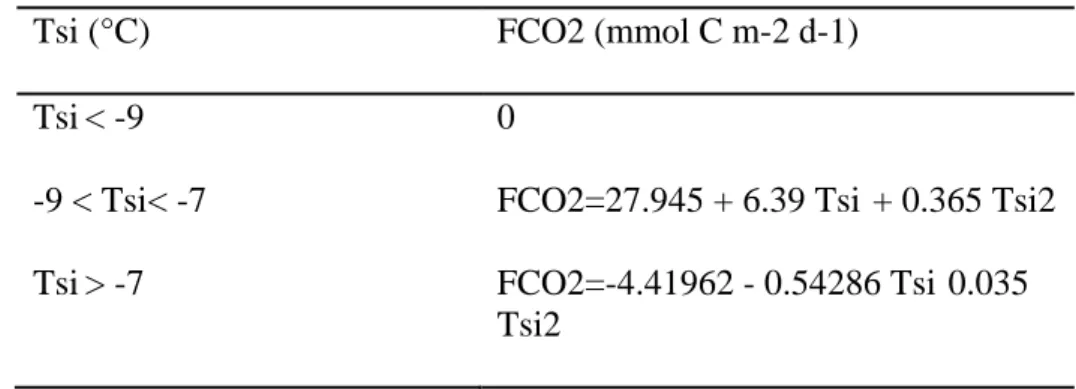
2.4. Air-ice CO2 flux/ice temperature relationship
183
Using field data, we calculated a relationship between CO2 fluxes (FCO2) over both first
184
year and multiyear ice as a function of sea ice temperature (Tsi) at 5cm depth (fig. 1a).
185
The regression is composed of two secondorder polynomial regressions valid between -186
9°C and -7°C and between -7°C and 0°C, respectively (table 1). 187
188
2.5. Description of the sea ice model
189
We used NEMO-LIM3 [Madec, 2008; Vancoppenolle et al., 2008] ocean-sea ice model 190
to scale in-situ measurements. NEMO (Nucleus for European Modelling of the Ocean) 191
is a widely used ocean model, while LIM3 (Louvain-la-Neuve Ice Model) is an 192
advanced large-scale sea ice model, carefully validated for both hemispheres. LIM3 is a 193
C-grid dynamic thermodynamic model, including the representation of the subgrid-scale 194
distributions of ice thickness, enthalpy and salinity as well as snow volume. Ice 195
dynamics are resolved using an elasto-visco-plastic rheology, following concepts of 196
Hunke and Dukowicz [1997]. Snow and sea ice thermodynamics include vertical 197
diffusion of heat with a formulation of brine thermal effect. There is also an explicit 198
formulation of brine entrapment and drainage. Sources and sinks of ice mass include 199
basal growth and melt, surface melt, new ice formation in open water, as well as snow 200
ice formation. In order to account for subgrid-scale variations in ice thickness, ice 201
volume and area are split into 5 categories of ice thickness. Thermodynamic (ice growth 202
and melt) as well as dynamical (rafting and ridging) processes control the redistribution 203
of ice state variables within the ice thickness categories. LIM3 is coupled to NEMO, a 204
hydrostatic, primitive equation finite difference ocean model running on a 2°×2°cos 205
grid called ORCA2. 206
207
We used the NEMO-LIM3 model output rather than satellite derivations of sea ice 208
temperature as the latter are presently not reliable in all conditions [Lewis, 2010]. In 209
comparison, we have reasonable confidence in the ice thickness, snow depth and 210
temperature simulated by LIM3, for the two following reasons. Firstly, a series of one-211
dimensional validations of the thermodynamic component of LIM3 was made over 212
various sites in both hemispheres [Vancoppenolle et al., 2007]. Vertical profiles of 213
temperature, salinity, as well as ice thickness and snow depth were found to be in close 214
agreement with field observations. In particular, the sea ice permeability transitions 215
seem to be quite well captured. Secondly, an extensive large-scale validation of LIM3, 216
forced by NCEP-NCAR daily reanalyses of meteorological data [Kalnay et al., 1996] 217
was performed [Vancoppenolle et al., 2008]. In the Antarctic, the simulated sea ice 218
concentration, thickness, drift and salinity and snow depth model fields are in 219
reasonable agreement with available observations. Because of errors in the wind 220
forcing, there is a low bias in ice thickness along the East side of the Antarctic 221
Peninsula, but this region is not of particular importance for the present analysis. 222
223
2.6. Computation of the snow-ice interface temperature and air-ice CO2 flux in the sea
224
ice model.
225
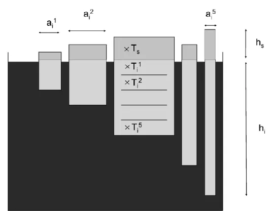
In LIM3 (fig.2), for each model grid cell, the sea ice thickness categories have a 226
relative coverage al (l = 1, …, 5). In each thickness category l, the sea ice is treated as a 227
horizontally uniform column with ice thickness hil and snow depth hsl. In order to
228
compute the vertical temperature profile, the sea ice in each category is vertically 229
divided into one layer of snow, with a midpoint temperature Ts and N=5 layers of sea
ice with midpoint temperatures Tikl (k = 1, …, 5). The snow and sea ice temperatures
231
are computed by the model by solving the heat diffusion equation. For the purpose of 232
the present study, we diagnose the ice-air interfacial temperature by assuming the 233
continuity of the heat conduction flux at the snow-ice interface: 234 N h k h k N h T k h T k T i s s i i s s s i i si 1 11 , (1) 235
where ki1 and ks are the thermal conductivities of the first sea ice layer and of snow,
236
respectively. The latter is done for each sea ice thickness category, which gives Tlsi (l=1,
237
…, 5). 238
The temperature at the snow-ice interface (fig.1b) is used to compute the air-ice CO2
239
flux in each sea ice thickness category, using the empirical relationship of 240 The fFigure1b: 241 ) ( 2 2 l si CO l CO F T F . (2) 242
Finally, the net, air-ice CO2 flux over all ice categories in the model grid cell is given
243 by: 244 245
5 1 2 2 l l CO l i ice air CO a F F . (3) 246Note that, as flooding affects the CO2 dynamics, points with surface flooding were
247
excluded in the present analysis. Snow-ice formation occurs in the model if the snow 248
load is large enough to depress the snow-ice interface under the sea level. The flooded 249
snow is transformed into ice by applying heat and mass conservation. 250
Following the setup detailed in Vancoppenolle et al. [2008], we conducted a hindcast 251
simulation of the Antarctic sea ice pack over 1976-2007, using a combination of daily 252
NCEP reanalyses of air temperature and winds [Kalnay et al., 1996] and of various 253
climatologies to compute the thermodynamic and dynamic forcings of the model. In 254
addition, the simulation includes the diagnostic air-ice CO2 flux. The time step is 1.6 h
255
for the ocean and 8 h for the sea ice. 256
257
3. Results and discussion
258
3.1. Changes in pCO2 of brines and air-ice CO2 fluxes during sea ice warming
259
3.1.1. pCO2 of brines
260
Sea ice-brine pCO2 decreased dramatically as sea ice warmed (fig. 1a) and the brines
261
shifted from a large CO2 over-saturation (pCO2 = pCO2(brines) – pCO2(air) = 525ppm)
262
during early spring (October) to a marked under-saturation (pCO2 = -335 ppm) during
263
summer (December). The sea ice brine pCO2 appears to be tightly related to sea ice
264
temperature. 265
As the ice temperature increases, ice crystals melt and salinity decreases accordingly. 266
We explored the relationships among brine pCO2, temperature and salinity by carrying
267
out a step-wise simulation of conservative dilution of early spring-time brine collected 268
during 2003/V1 cruise during warming at thermal brine-ice equilibrium. In details, (i) 269
we calculated brine salinity at a given temperature according to the relationship of Cox 270
and Weeks [1983]; (ii) we normalized mean TA and DIC to a salinity of 35 (TA35, and
271
DIC35, respectively) for the two coldest brines collected during 2003/V1 cruise; (iii) we
272
computed TAt and DICt at a given temperature, t (and related salinity) assuming a
273
conservative behaviour of TA and DIC; and (iv) computed the brine pCO2 for each
274
temperature from TAt and DICt, using CO2 acidity constants of Dickson and Millero
[1987]. Here we assume that these constants are valid for the range of temperatures and 276
salinities encountered within the sea ice [Delille et al., 2007; Papadimitriou et al., 277
2004]. The resulting pCO2 - temperature relationship is shown in fig. 1a (red dashed
278
curve). The dilution effect largely encompasses the thermodynamic effect of 279
temperature increase on pCO2 and the pattern of observed pCO2 matches the theoretical
280
variation related to both processes. This suggests that a large part of the spring pCO2
281
drawdown is driven by the dilution of brines associated with the melting of ice crystals 282
as temperature increases. Conversely, the over-saturation observed at the end of winter 283
can result from brine concentration during sea ice growth and cooling. 284
3.1.2. CO2 fluxes
285
While air-ice CO2 fluxes were not detectable below -8°C (fig.1b) , we observed
286
positive fluxes up to +1.9 mmol m-2 d-1 between -8 and -6 °C (where a positive flux 287
corresponds to a release of CO2 from the ice to the atmosphere). Above -6°C, air-ice
288
CO2 fluxes decrease down to –5.2 mmol m-2 d-1 in parallel with the increase of
289
temperature. These fluxes are of the same order of magnitude as the fluxes reported by 290
Nomura et al. [2013] over land fast ice. Higher sinks (negative fluxes:-6.6 to -18.2
291
mmol m-2 d-1 ) have been reported in Antarctica [Zemmelink et al., 2006]. These were 292
carried out using eddy covariance over a slush ice - a mixture of melting snow, ice and 293
flooding seawater covering the sea ice. Note, however, that computations of Zemmelink 294
et al. [2006] should be considered with caution, since they did not take into account at
295
the time proper corrections required for open-path CO2 analyser in cold temperature
296
[Burba et al., 2008]. 297
3.2. Assessment of atmospheric CO2 uptake by Antarctic sea ice from the relative
298
contribution of processes controlling sea ice pCO2
299
Impurities expulsion (that might be enhanced for CO2 compared to salt [Loose et al.,
300
2009]), changes in brines concentration, precipitation or dissolution of carbonate 301
[Anderson and Jones, 1985; Delille et al., 2007; Papadimitriou et al., 2004; 302
Papadimitriou et al., 2007; Rysgaard et al., 2007], abiotic release or uptake of gaseous
303
CO2, primary production and respiration all contribute to CO2 dynamics [Delille et al.,
304
2007; Søgaard et al., 2013] in sea ice. In this section we will describe those processes 305
and provide an estimate of their relative contribution to spring and summer pCO2
306
changes in sea ice. We estimated the potential maximal individual impact of 307
thermodynamic, chemical and biological processes (temperature increase and related 308
dilution, carbonate dissolution and primary production) to the spring-summer decrease 309
of pCO2 (table 2). The variations are computed from the conditions of temperature, bulk
310
ice salinity, TA35 and pCO2 (-7.2°, 5.4, 791 µmol kg-1, 724 ppm, respectively)
311
corresponding to the average of the two coldest conditions encountered during the 312
2003/V1 (coldest end term of the solid curve in figure 1a) and ISPOL cruises. Related 313
changes during the spring to summer transition are discussed in the sections below. 314
3.3. Changes in brines concentration
315
In autumn and winter, decrease of temperature leads to the concentration of solutes in 316
brines inclusions which induce high pCO2 within sea ice brines as observed in figure 1a.
317
In spring and summer, as the temperature increases, the melt of ice crystals and the 318
subsequent dilution of the brines promote a decrease of the sea ice brine pCO2. For all
319
our cruises, temperature increased from -7.2 °C to -1.3°C (corresponding to an increase 320
of 5.9°C in table Table 1: Fit expression of the relationship between CO2 fluxes (FCO2) 321
over both first year and multiyear ice as a function of sea ice temperature (Tsi) at 5cm 322
depth used for reconstructing air-ice CO2 fluxes from the NEMO-LIM3 model as it 323
appears in figure 1b (solid curve). Number of samples, mean error, standard error, root-324
mean-square error, coefficient of determination were 21, -0.099 mmol C m-2 d-1, 0.995 325
mmol C m-2 d-1, 0.953, 0.728, respectively. 326
Tsi (°C) FCO2 (mmol C m-2 d-1)
Tsi< -9 0
-9 < Tsi< -7 FCO2=27.945 + 6.39 Tsi + 0.365 Tsi2
Tsi> -7 FCO2=-4.41962 - 0.54286 Tsi 0.035
Tsi2 327
328 329
Table 2) with a decrease of the brine salinity from 117.1 to 23.5, (corresponding to a 330
salinity change of -94 in table Table 1: Fit expression of the relationship between CO2 331
fluxes (FCO2) over both first year and multiyear ice as a function of sea ice temperature 332
(Tsi) at 5cm depth used for reconstructing air-ice CO2 fluxes from the NEMO-LIM3 333
model as it appears in figure 1b (solid curve). Number of samples, mean error, standard 334
error, root-mean-square error, coefficient of determination were 21, -0.099 mmol C m-2 335
d-1, 0.995 mmol C m-2 d-1, 0.953, 0.728, respectively. 336
Tsi (°C) FCO2 (mmol C m-2 d-1)
Tsi< -9 0
-9 < Tsi< -7 FCO2=27.945 + 6.39 Tsi + 0.365 Tsi2
Tsi> -7 FCO2=-4.41962 - 0.54286 Tsi 0.035
Tsi2 337
338 339
Table 2) according to relationships of Cox and Weeks [1983]. 340
The decrease in salinity, related to the rise of temperature, leads to the dilution of DIC 341
and TA. This induces a computed pCO2 drop of 684 ppm (table Table 1: Fit expression
342
of the relationship between CO2 fluxes (FCO2) over both first year and multiyear ice as 343
a function of sea ice temperature (Tsi) at 5cm depth used for reconstructing air-ice CO2 344
fluxes from the NEMO-LIM3 model as it appears in figure 1b (solid curve). Number of 345
samples, mean error, standard error, root-mean-square error, coefficient of 346
determination were 21, -0.099 mmol C m-2 d-1, 0.995 mmol C m-2 d-1, 0.953, 0.728, 347
respectively. 348
Tsi (°C) FCO2 (mmol C m-2 d-1)
Tsi< -9 0
-9 < Tsi< -7 FCO2=27.945 + 6.39 Tsi + 0.365 Tsi2
Tsi> -7 FCO2=-4.41962 - 0.54286 Tsi 0.035
Tsi2 349
350 351
Table 2), using the CO2 dissociation constants of Mehrbach et al. [1973] refitted by
352
Dickson and Millero [1987]. Brine dilution by internal melting appears to account for a
353
significant part of the observed pCO2 spring drawdown.
354
3.4. Primary production
While sympagic algae are still active in autumn and winter, their photosynthetic rate 356
should be limited by light availability, low temperatures, high salinity and restricted 357
space for growth [Arrigo et al., 1997; Mock, 2002], and this contribution to the DIC 358
normalized to a constant salinity of 35 (DIC35) winter removal observed in the figure 3
359
is therefore likely small. 360
Estimating primary production in sea ice – and the related impact on pCO2 - is
361
challenging. We assumed the overall sea ice primary production prior to and during the 362
ISPOL cruise corresponded to the autotrophic organic carbon (OCautotroph) standing stock
363
in the ice at the end of the ISPOL cruise. This autotrophic organic carbon was estimated 364
from Chl a measurements (at 6 depths) presented in [Lannuzel et al., 2013] and a 365
C:Chla ratio of 83. This ratio was determined by comparing Chl a concentration and 366
OCautotroph content derived from abundance and biovolume of autotrophic organisms
367
measured from inverted and epifluorescence microscopy observations, and 368
carbon:volume conversion factors [Hillebrand et al., 1999; Menden-Deuer and Lessard, 369
2000]. 370
The autotrophic organic carbon amount could be underestimated because it does not 371
take into account losses of autotrophic organic carbon (i.e. mortality, exchange with the 372
underlying seawater). On the other hand, we neglected the part of autotrophic 373
community originating from organisms trapped during sea ice growth and autumnal 374
primary production. At the end of the ISPOL cruise, the mean Chl a concentration was 375
3.7 µg kg-1 of bulk ice, which corresponds to an OCautotroph standing stock of 309 µgC
376
kg-1 of bulk ice. The build up of the OCautotroph standing stock would correspond to an
377
uptake of DIC of 25.8 µmol kg-1 in bulk ice and an increase of TA of 4.1 µmol kg-1 of 378
bulk ice, according to the Redfield-Ketchum-Richards stoichiometry of biosynthesis 379
[Redfield et al., 1963; Richards, 1965]. With the volume of brines derived from the 380
equations of Cox and Weeks [1975], revisited by Eicken [2003], this leads to a DIC 381
decrease of 669 µmol kg-1 of brines and a TA increase of 107 µmol kg-1 of brines (table 382
2) and a subsequent decrease of the of brines pCO2 of 639 ppm (table 2). The build up
383
of the OCautotroph standing stock would also correspond to a primary production of 0.26
384
gC m-2 considering an ice thickness of 90 cm (average ice thickness during the ISPOL 385 survey). 386 387 3.5. Calcium carbonate 388
The figure 3 provides insights on the processes occurring within sea ice prior and during 389
our surveys. We plotted normalized DIC35 versus normalized TA (TA35) in order to
390
distinguish which processes, other than dilution/concentration and temperature changes, 391
control the carbonate system. Normalization removes the influence of
392
dilution/concentration, while temperature changes do not affect DIC and TA. The 393
biogeochemical processes that can potentially affect DIC35 and TA35 are reported as
394
solid bars. TA35 and DIC35 of brines in spring are significantly lower than in the
395
underlying water. Differences between brines and the underlying water decrease in 396
summer. TA35 and DIC35 in both spring and summer are remarkably well correlated
397
with a slope of 1.2.Carbonate dissolution/precipitation best explain the observed trend, 398
although the theoretical slope should be 2. Such a discrepancy might be due to uptake of 399
gaseous CO2 (from bubbles or the atmosphere) combined with carbonate dissolution,
400
mixing with underlying water owing to internal convection, or enhanced gas expulsion 401
[Golden et al., 1998; Loose et al., 2009; Weeks and Ackley, 1986] . The low TA35 value
observed during 2003/V1 cruise suggests that carbonate precipitation occurred within 403
sea ice prior to the cruise. 404
Rysgaard et al. [2007] suggested that precipitation of calcium carbonate in sea ice can
405
act as a significant sink for atmospheric CO2. However, there are still some crucial gaps
406
in the current understanding of carbonate precipitation in sea ice. In particular available 407
field experiments hardly addressed the timing and conditions of carbonate precipitation 408
in natural sea ice. Knowing these conditions is nevertheless crucial to assess the role 409
played by sea ice carbonate precipitation as a sink or source of CO2 for the atmosphere.
410
In order to bring some attention on the need to better constrain CaCO3 precipitation in
411
natural sea ice, we consider below different scenarios of CaCO3 precipitation and
412
explore how air-ice CO2 fluxes depend on the condition of CaCO3 precipitation.
413
Furthermore, the fate of carbonate precipitates is a good illustration of how intricate the 414
links between biogeochemical and physical sea ice processes are (fig. 4). Based on field 415
studies, "excess" TA in the water column during sea ice melting was attributed to the 416
dissolution of calcium carbonate precipitated in brines and released into the underlying 417
water [Jones et al., 1983; Rysgaard et al., 2007]. Precipitation of calcium carbonate as 418
ikaite (CaCO3.6H2O) crystals have been observed both in the Arctic and the Antarctic
419
sea ice [Dieckmann et al., 2008; Dieckmann et al., 2010; Geilfus et al., 2013; Rysgaard 420
et al., 2007; Rysgaard et al., 2013; Søgaard et al., 2013].
421
If carbonate precipitate in high salinity – low temperature conditions, such precipitation 422
would likely take place in late autumn or winter in the upper layers of sea ice while 423
brines channels are closed (fig. 4B). This precipitation produces CO2. If brines channels
424
are closed, this CO2 is not transported elsewhere. For instance Killawee et al. [1998]
425
and Tison et al. [2002] already observed CO2 rich bubbles in artificial sea ice and
suggested that they could be issued from carbonate precipitation. During spring internal 427
melting, dissolution of carbonate solids formed in fall and winter should consumes CO2
428
in the same amount as it was produced by precipitation. The net uptake of 429
atmospheric/sea water CO2 related to the production and dissolution of carbonate in that
430
case would be nil over the period. 431
In the opposite, the phase diagram of Assur [1958] and the work of Richardson [1976], 432
suggest that ikaite could precipitate at relatively high temperature (-2.2°C) and low 433
salinity. Under these conditions, carbonate precipitation might potentially take place in 434
the skeletal layer (the lamellar ice-water interface, a relatively open system) during sea 435
ice growth (fig. 4F). At the ice-water interface, the segregation of impurities enhances 436
CO2 concentration at the ice-water interface during ice growth [Killawee et al., 1998]
437
and acts as a source of CO2 for the underlying layer. CO2 produced by the precipitation
438
can either be expelled to the underlying water layer (fig. 4C) or released to the 439
atmosphere, especially in young thin permeable sea ice [Geilfus et al., 2013]. A crucial 440
issue is the fate of carbonate solids formed in the skeletal layer. They can either a) sink 441
(fig. 4F) in the underlying layer faster than the CO2 rich brines (fig. 4 D). In that case,
442
carbonate precipitation act as a net source of CO2 for the atmosphere, especially if some
443
CO2 rich brines trapped within sea ice are connected to the atmosphere in spring and
444
summer (fig. 4E). b) Carbonate solids may sink at the same rate than the brines that 445
transport produced CO2 with negligible impact on DIC budget of the water column and
446
the impact for the atmosphere is nil. c) Carbonate solids remain trapped in the tortuosity 447
of the skeletal layer while CO2 produced by the precipitation is expelled to the
448
underlying water with the brines (fig. 4 C) and entrained towards deep layers due to the 449
high density of brines. The dissolution of trapped carbonate solids in spring and summer 450
triggered by temperature increases and related salinity decreases, would consume CO2
451
and drive CO2 uptake within the ice. In that case carbonate precipitation acts as a sink
452
for atmospheric CO2. However Papadimitriou et al. [2013] showed recently that at
-453
2.2°C carbonate precipitation can occur only in low pCO2 conditions, that are
454
uncommon below sea ice during sea ice formation. 455
Taking into account the estimates of the saturation state of ikaite as a function of brine 456
pCO2 and temperature provided by Papadimitriou et al. [2013] and taking into account
457
the pCO2 vs temperature relationship of the figure 1a, it seems reasonable that the
458
threshold of saturation of ikaite for brine corresponds to temperature ranging between -459
5°C and -6°C. So when the ice cools down, carbonate precipitation can potentially 460
develop below -5°C. If the bulk salinity of ice is above 5, then at -5°C, the brine volume 461
is above 5% [Cox and Weeks, 1983; Eicken, 2003] and ice is permeable [Golden et al., 462
1998]. In these conditions, fluids still percolate and transport CO2 while solid particles
463
remain trapped due to the tortuosity of the ice matrix. This corresponds to the previous 464
(c) scenario. 465
This leads to the segregation between carbonate precipitates, which remain trapped 466
within sea ice while the CO2 produced is expelled to the underlying water with brines.
467
Such a mechanism could act as an efficient pump of CO2 from the atmosphere. The
468
expulsion of brines enriched in CO2 leads to the formation of dense water that sinks
469
rapidly during sea ice growth. The sinking of dense water is the main driver of deep-470
water formation and is potentially an efficient CO2 sequestration pathway. Numerous
471
vertical distributions profiles of TA below sea ice have revealed the signature of 472
carbonate precipitation [Weiss et al., 1979]. When sea ice melts during spring and 473
summer, trapped carbonate solids dissolve as the result of the combined increase of 474
temperature and decrease of salinity either within sea ice or in the underlying water. 475
This dissolution of carbonate solids observed by Jones et al. [1983] leads to a decrease 476
of pCO2 and might act as an efficient and significant sink of CO2 according to
477
observations and models [Rysgaard et al., 2011; Rysgaard et al., 2012; 2007; Søgaard 478
et al., 2013]. However, as underlined before, part of that process might not be a net
479
annual sink if carbonate precipitate in permeable sea ice, and that the produced CO2
480
degasses to the atmosphere [Geilfus et al., 2013]. 481
Low values of DIC35 and TA35 in brines collected in early spring in cold sea ice (fig. 3)
482
indicate that carbonate precipitation occurred within brines prior to the 2003/V1 cruise, 483
further eastwards. The imprint of carbonate precipitation is well marked, leading to a 484
decrease of 65 % of TA35 in brines, compared to the underlying water(fig. 3). Such
485
difference would correspond to the precipitation of carbonate of about 2038 µmol kg-1 486
from the brines, assuming the effect of fall and winter microbial activity on TA is 487
negligible. Carbonate precipitation will reduce the DIC35 and increase pCO2 as the brine
488
salinity increases during ice growth. This will contribute to the winter over-saturation of 489
CO2. If we assume that the carbonate solids remain trapped within the ice and no CO2 is
490
stored in the gaseous phase within sea ice during the cooling processes, then spring 491
dissolution would reduce pCO2 by about 583 ppm (table Table 1: Fit expression of the
492
relationship between CO2 fluxes (FCO2) over both first year and multiyear ice as a 493
function of sea ice temperature (Tsi) at 5cm depth used for reconstructing air-ice CO2 494
fluxes from the NEMO-LIM3 model as it appears in figure 1b (solid curve). Number of 495
samples, mean error, standard error, root-mean-square error, coefficient of 496
determination were 21, -0.099 mmol C m-2 d-1, 0.995 mmol C m-2 d-1, 0.953, 0.728, 497
respectively. 498
Tsi (°C) FCO2 (mmol C m-2 d-1)
Tsi< -9 0
-9 < Tsi< -7 FCO2=27.945 + 6.39 Tsi + 0.365 Tsi2
Tsi> -7 FCO2=-4.41962 - 0.54286 Tsi 0.035
Tsi2 499 500 501 Table 2). 502
However, the observed decrease in TA35 due to carbonate precipitation corresponds
503
theoretically to a removal of 30 % of DIC35, while the overall decrease of DIC35 reaches
504
70% at the coldest temperature (fig. 3). Thus, about 40% of DIC35 reduction has to be
505
ascribed to either autumnal/winter primary production or CO2 transfer to the gas phase
506
within the brines or enhanced gas expulsion compared to salt [Loose et al., 2009]. For 507
instance, Geilfus et al. [2013] report significant release of CO2 from the ice to the
508
atmosphere as a result of solutes expulsion during early stages of ice formation. 509
3.6. First order assessment of air-ice CO2 transfers over Antarctic sea ice
510
The potential air-ice CO2 transfers related to sea ice physical and biogeochemical
511
processes were assessed by considering a homogeneous 90 cm thick sea ice cover in 512
equilibrium with the atmosphere and isolated from exchange with the underlying water. 513
The sea ice thickness value is the mean observed during the ISPOL experiment and is 514
low compared to the values generally observed in the Weddell Sea and elsewhere [Haas 515
et al., 2003; Timmermann et al., 2002]. Temperature, salinity and δ18O data [Tison et 516
al., 2008] suggest that low exchanges occurred between sea ice and the underlying layer
during the ISPOL experiment . We assumed that sea ice was initially in equilibrium 518
with the atmosphere (pCO2 = 370 ppm), and we applied the biogeochemically driven
519
DIC and TA changes of table Table 1: Fit expression of the relationship between CO2 520
fluxes (FCO2) over both first year and multiyear ice as a function of sea ice temperature 521
(Tsi) at 5cm depth used for reconstructing air-ice CO2 fluxes from the NEMO-LIM3 522
model as it appears in figure 1b (solid curve). Number of samples, mean error, standard 523
error, root-mean-square error, coefficient of determination were 21, -0.099 mmol C m-2 524
d-1, 0.995 mmol C m-2 d-1, 0.953, 0.728, respectively. 525
Tsi (°C) FCO2 (mmol C m-2 d-1)
Tsi< -9 0
-9 < Tsi< -7 FCO2=27.945 + 6.39 Tsi + 0.365 Tsi2
Tsi> -7 FCO2=-4.41962 - 0.54286 Tsi 0.035
Tsi2 526
527 528
Table 2 (expressed per kilogram of bulk ice), and then computed the air-ice CO2
529
transfers required to restore equilibrium. We used the brine volume values computed 530
from the equations of Cox and Weeks [1975] revisited by Eicken [2003] and mean 531
conditions observed during the two last ISPOL stations (mean sea ice temperature: -532
1.3°C, mean brine salinity: 24, mean bulk ice salinity: 3.8, mean TA: 1667 µmol kg -1 of 533
brines). For the uptake owing to temperature change and related dilution effect, we 534
considered a temperature increase from -7.2 to -1.3 °C corresponding to the range of 535
observations during the 2003/V1 and ISPOL cruises, salinity decrease from 117 to 24 536
and decrease of TA from 8135 to 1667 µmol kg-1 of brinesso that TA35 remains
537
constant. 538
For an Antarctic first-year sea ice surface area of 14×106 km2 [Comiso, 2003], the 539
corresponding upscaled overall CO2 uptake due to those cumulated three processes
540
(table 3) is 0.024 PgC for Spring-Summer. 541
3.7. Comparison of the significance of the main processes on CO2 uptake
542
Tables 2 and 3 provide some insights on the relative contribution of the three main 543
processes (increase of temperature and related dilution, primary production and 544
dissolution of carbonate solids) to the pCO2 drawdown and the uptake of atmospheric
545
CO2. It must keep in mind that the assessment of the contribution of primary production
546
is less robust than the other assessments. As observed by Delille et al. [2007] in 547
Antarctic land fast ice, the impact on pCO2 of warming and related dilution is similar to
548
those of dissolution of carbonate solids. The contribution of primary production is only 549
slightly lower (tables 2). In terms of CO2 uptake, the contribution of primary production
550
represents only 45 % of the contribution of each other process, but it still significant. In 551
contrast Søgaard et al. [2013] in subarctic land fast suggest that the contribution of 552
primary production to the uptake of atmospheric CO2 is pretty small compare to the
553
other processes. However, these differences should reflect the differences in primary 554
production between different areas. 555
556
3.8. Assessment of atmospheric CO2 uptake by Antarctic sea ice from fluxes:sea ice
557
temperature relationship in a 3D model.
558
We measured CO2 fluxes over widespread sea ice without biologically active surface
559
communities. Previous eddy correlation CO2 fluxes measurements were carried out over
areas covered by particular surface environments, namely melt ponds and slush 561
[Semiletov et al., 2004; Zemmelink et al., 2006]. Slush is known to hosts a highly 562
productive algae community [Legendre et al., 1992]. Sea ice surface communities 563
benefit from high light levels and from nutrients from seawater flooding as snow 564
loading or sea ice rafting depress the ice surface below the freeboard. Such surface 565
flooding occurs over 15-30% of the ice pack in Antarctica [Wadhams et al., 1987]. 566
These surface communities exhibit photosynthetic rates comparable to those of open 567
ocean Antarctic phytoplankton [Lizotte and Sullivan, 1992] and might be responsible for 568
the majority of sea surface productivity in Antarctic sea ice [Legendre et al., 1992]. 569
They easily exchange CO2 with the atmosphere through the porous snow cover and can
570
potentially enhance significantly the estimate for CO2 uptake by the sea ice cover given
571
below. 572
In a heterogeneous environment like sea ice, the small spatial resolution of the chamber 573
CO2 flux measurements allows a consistent comparison with pCO2 within the ice. The
574
pCO2 gradient between the atmosphere and the brines in the sea ice top layer is the main
575
driver of CO2 fluxes. The CO2 fluxes are consistent with the saturation level of CO2 in
576
the brines. No CO2 flux was detected below -10°C suggesting that sea ice was then
577
virtually impermeable to CO2 exchange (fig. 1b). At a temperature of ~ -7°C, the low
578
permeability of the ice results in weak net CO2 fluxes despite elevated pCO2. As the
579
temperature increases, pCO2 of the ice decreases and sea ice shifts from a transient CO2
580
source to a sink. 581
The fluxes are modulated by factors like sea ice temperature, and snow and ice structure 582
[Geilfus et al., 2012; Nomura et al., 2010; Nomura et al., 2013]. While snow allows 583
exchange of gases with the atmosphere [Albert et al., 2002; Massman et al., 1997; 584
Takagi et al., 2005], very low to nil fluxes were observed after the formation of lenses
585
of superimposed ice above sea ice (diamonds in figure 1b) that was detected at the 586
sampling site and elsewhere during ISPOL cruise [Nicolaus et al., 2009]. Superimposed 587
ice forms after a strong snow melt event when percolating freshwater refreezes at the 588
contact of proper sea ice [Haas et al., 2001]. As freshwater ice, the superimposed ice is 589
impermeable to gas transport [Albert and Perron, 2000]. The formation of 590
superimposed ice at the top of sea ice observed at certain stations during ISPOL cruise 591
is the best candidate to explain the inhibition of air-ice CO2 fluxes at those stations.
592
During superimposed ice events, ongoing strong dilution of the brine by the melting sea 593
ice was decreasing brine pCO2. Development of superimposed ice impeded CO2 transfer
594
from the atmosphere to the sea ice that normally should drive pCO2 values toward the
595
atmospheric concentration. As a result drastic decreases of brine pCO2 down to 30 ppm
596
were observed during superimposed ice events. This highlights the role of CO2 invasion
597
from the atmosphere that balances the summer pCO2 drawdown sustained by dilution
598
and primary production, and maintains sea ice pCO2 above 100 ppm.
599
Despite the effect of snow and ice structure on fluxes, sea ice temperature appears to 600
exerts a crucial control on both sea ice pCO2 gradient, gas transfer through permeability,
601
and ultimately on CO2 transfer at the air-ice interface (fig 1b). We therefore derived an
602
empirical relationship between CO2 flux and sea ice temperature (fig. 1b) allowing the
603
reconstruction of CO2 flux fields (fig. 5) using sea ice temperature, concentration and
604
coverage from the NEMO-LIM3 large-scale sea ice-ocean model [Madec, 2008; 605
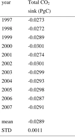
Vancoppenolle et al., 2008]. Spring and summer air-ice CO2 fluxes were estimated from
606
1997 to 2007 for non-flooded areas with ice concentration above 65% (fig. 6), 607
corresponding to the range of sea ice concentration encountered during sampling. This 608
up-scaling suggests that Antarctic sea ice cover pumps 0.029 PgC of atmospheric CO2
609
(table 4) into the ocean during the spring-summer transition. 610
This assessment corroborates the first order independent assessment derived from pCO2
611
dynamics relative to each main process (see previous section). Both CO2 sink estimates
612
most probably underestimate the uptake of CO2 over Antarctic sea ice as they do not
613
account for (1) areas with sea ice concentration < 65 %, (2) flooded areas, (3) surface 614
communities that may significantly enhance CO2 uptake.
615
616
4. Conclusion
617
The elevated sea ice pCO2 in winter results from an intricate superimposition of
618
counteracting processes: those increasing pCO2 such as brine concentration and
619
carbonate precipitation, and those decreasing pCO2 such as enhanced gas expulsion,
620
autumnal primary production, temperature decrease, CO2 transfer to the gaseous phase.
621
In spring, we observed a sharp decrease of pCO2 that is tightly related to sea ice melting
622
and related brine dilution. We also show that carbonate dissolution could induce pCO2
623
changes comparable to those attributed to dilution. In summer, as sea ice becomes 624
isothermal, dilution effects level off. At that stage, uptake of atmospheric CO2 and
625
mixing with underlying water (with pCO2 values ranging from 380 to 430 ppm) should
626
maintain pCO2 at or above the saturation level. However, sustained primary production
627
appears to be large enough to maintain low pCO2 within the sea ice. One should note
628
that we did not address CO2 uptake from the underlying to the ice driven by bottom
629
sympagic communities and CO2 transfer from the underlying water to the atmosphere
through the ice that are considered insignificant [Loose et al., 2011; Rutgers van der 631
Loeff et al., 2014].
632
These processes act as sink for atmospheric CO2. Using the relative contribution of the
633
main processes driving pCO2 in sea ice we derived an uptake of 0.024 PgC for spring
634
and summer. This assessment corroborates the estimate from in situ CO2 flux
635
measurements scaled with the ice temperature simulated with the NEMO-LIM3 model 636
that is assessed to 0.029 PgC. Both assessments compare favourably with the 637
assessments of Rysgaard et al. [2011] of 0.019 and 0.052 PgC yr-1 for the CO2 fluxes
638
over the whole southern ocean, respectively “without” and “with”CaCO3 formation in
639
sea ice. 640
We consider that the fluxes derived from the NEMO-LIM3 are the best estimate to date 641
of the uptake of atmospheric CO2 by Antarctic sea ice in spring and summer.
642
Accordingly, sea ice provides an additional significant sink of atmospheric CO2 in the
643
Southern Ocean up to 58 % of the estimated net uptake of the Southern Ocean south of 644
50°S (0.05 PgC yr-1) [Takahashi et al., 2009]. Antarctic pack ice appears to be a 645
significant contributor of CO2 fluxes in the southern ocean. We believe that our
646
approach is conservative since we excluded areas with ice concentration below 65% and 647 flooded zones. 648 649
Acknowledgments
650The authors appreciated the kindness and efficiency of the crews of R.S.V Aurora 651
Australis, R.V. Polarstern and R.V. N.B.Palmer. We are grateful to Tom Trull, Steve
Ackley and two anonymous reviewers for their useful comments that improved the 653
quality of the manuscript. This research was supported by the Belgian Science Policy 654
(BELCANTO projects, contract SD/CA/03A), the Belgian French Community 655
(SIBCLIM project), the F.R.S.-FNRS and the Australian Climate Change Science 656
Program. NXG received a PhD grant from the Fonds pour la Formation à la Recherche 657
dans l’Industrie et l’Agriculture and now received financial support from the Canada 658
Excellence Research Chair (CERC) program. BD is a research associate of the F.R.S.-659
FNRS. VS benefits from a COFUND Marie Curie fellowship “Back to Belgium Grant”. 660
Supplemental data used to produce figures are freely available at the address 661
www.co2.ulg.ac.be/data/Delille_et_al_supplemental_data.xlsx. This is MARE 662 contribution XXX. 663 664
References
665 666Albert, M. R., A. M. Grannas, J. Bottenheim, P. B. Shepson, and F. E. Perron (2002), 667
Processes and properties of snow-air transfer in the high Arctic with application to 668
interstitial ozone at Alert, Canada, Atmos. Environ., 36(15-16), 2779-2787. 669
Albert, M. R., and F. E. Perron (2000), Ice layer and surface crust permeability in a 670
seasonal snow pack, Hydrological Processes, 14(18), 3207-3214. 671
Anderson, L. G., and E. P. Jones (1985), Measurements of total alkalinity, calcium and 672
sulfate in natural sea ice, J. Geophys. Res., 90(C5), 9194-9198, 673
doi:10.1029/JC090iC05p09194. 674
Arrigo, K. R. (2003), Primary production in sea ice, in Sea ice: an introduction to its 675
physics, chemistry, biology and geology, edited by D. N. Thomas and G. Dieckmann,
676
pp. 143-183, Blackwell Science, Oxford. 677
Arrigo, K. R., D. L. Worthen, M. P. Lizotte, P. Dixon, and G. Dieckmann (1997), 678
Primary production in antarctic sea ice, Science, 276, 394-397, 679
doi:10.1126/science.276.5311.394. 680
Assur, A. (1958), Composition of sea ice and its tensile strength, in Arctic Sea Ice, 681
edited, pp. 106-138, National Academy of Sciences-National Research Council. 682
Buckley, R. G., and H. J. Trodahl (1987), Thermally driven changes in the optical 683
properties of sea ice, Cold Reg. Sci. Technol., 14(2), 201-204. 684
Burba, G., D. K. McDermitt, A. Grelle, D. J. Anderson, and L. Xu (2008), Addressing 685
the influence of instrument surface heat exchange on the measurements of CO2 flux
from open-path gas analyzers, Global Change Biology, 14(8), 1854-1876, 687
doi:10.1111/j.1365-2486.2008.01606.x. 688
Comiso, J. C. (2003), Large-scale characteristics and variability of the global sea ice 689
cover, in Sea ice: an introduction to its physics, chemistry, biology and geology, edited 690
by D. N. Thomas and G. Dieckmann, pp. 112-142, Blackwell Science, Oxford. 691
Copin-Montégut, C. (1988), A new formula for the effect of temperature on the partial 692
pressure of carbon dioxide in seawater, Mar. Chem., 25(1), 29-37. 693
Cox, and W. Weeks (1983), Equations for determining the gas and brine volumes in 694
sea-ice samples, J. Glaciol., 29(102), 306-316. 695
Cox, G. F. N., and W. F. Weeks (1975), Brine drainage and initial salt entrapment in 696
sodium chloride iceRep., 85 pp. pp. 697
Delille, B., B. Jourdain, A. V. Borges, J. L. Tison, and D. Delille (2007), Biogas (CO2,
698
O2, dimethylsulfide) dynamics in spring Antarctic fast ice, Limnol. Oceanogr., 52(4),
699
1367-1379, doi:10.4319/lo.2007.52.4.1367. 700
Dickson, A. G., and F. J. Millero (1987), A comparison of the equilibrium constants for 701
the dissociation of carbonic acid in seawater media, Deep-Sea Res. Part I Oceanogr. 702
Res. Pap., 34, 1733-1743, doi:10.1016/0198-0149(87)90021-5.
703
Dieckmann, G. S., G. Nehrke, S. Papadimitriou, J. Göttlicher, R. Steininger, H. 704
Kennedy, D. Wolf-Gladrow, and D. N. Thomas (2008), Calcium carbonate as ikaite 705
crystals in Antarctic sea ice, Geophys. Res. Lett., 35(L08501), 706
doi:10.1029/2008GL033540. 707
Dieckmann, G. S., G. Nehrke, C. Uhlig, J. Göttlicher, S. Gerland, M. A. Granskog, and 708
D. N. Thomas (2010), Ikaite (CaCO3*6H2O) discovered in Arctic sea ice, The
709
Cryosphere, 4(2), 227-230, doi:10.5194/tc-4-227-2010.
710
Eicken, H. (2003), From the microscopic, to the macroscopic, to the regional scale: 711
growth, microstructure and properties of sea ice, in Sea ice: an introduction to its 712
physics, chemistry, biology and geology, edited by D. N. Thomas and G. Dieckmann,
713
pp. 22-81, Blackwell Science, Oxford. 714
Frankignoulle, M. (1988), Field measurements of air-sea CO2 exchange, Limnol.
715
Oceanogr., 33, 313-322.
716
Geilfus, N. X., G. Carnat, G. S. Dieckmann, N. Halden, G. Nehrke, T. Papakyriakou, J. 717
L. Tison, and B. Delille (2013), First estimates of the contribution of CaCO3 718
precipitation to the release of CO2 to the atmosphere during young sea ice growth, 719
journal of geophysical Research - Oceans, 118(1-12), doi:10.1029/2012JC007980.
720
Geilfus, N. X., G. Carnat, T. Papakyriakou, J. L. Tison, B. Else, H. Thomas, E. 721
Shadwick, and B. Delille (2012), Dynamics of pCO2 and related air-ice CO2 fluxes in
722
the Arctic coastal zone (Amundsen Gulf, Beaufort Sea), Journal of Geophysical 723
Research C: Oceans, 117(2), doi:10.1029/2011JC007118.
724
Gleitz, M., M. R. v.d.Loeff, D. N. Thomas, G. S. Dieckmann, and F. J. Millero (1995), 725
Comparison of summer and winter in organic carbon, oxygen and nutrient 726
concentrations in Antarctic sea ice brine, Mar. Chem., 51(2), 81-91, doi:10.1016/0304-727
4203(95)00053-T. 728
Golden, K. M., S. F. Ackley, and V. I. Lytle (1998), The percolation phase transition in 729
sea ice, Science, 282(5397), 2238-2241, doi:10.1126/science.282.5397.2238. 730
Gosink, T. A., J. G. Pearson, and J. J. Kelley (1976), Gas movement through sea ice, 731
Nature, 263(2), 41-42, doi:10.1038/263041a0.
732
Gran, G. (1952), Determination of the equivalence point in potentiometric titration, part 733
II, Analyst, 77, 661-671. 734
Haas, C., D. N. Thomas, and J. Bareiss (2001), Surface properties and processes of 735
perennial Antarctic sea ice in summer, J. Glaciol., 47(159), 613-625. 736
Haas, C., D. N. Thomas, and G. Dieckmann (2003), Dynamics versus thermodynamics: 737
the sea ice thickness distribution, in Sea ice: an introduction to its physics, chemistry, 738
biology and geology, edited, pp. 82-111, Blackwell Science, Oxford.
739
Hillebrand, H., C. D. Durselen, D. Kirschtel, U. Pollingher, and T. Zohary (1999), 740
Biovolume calculation for pelagic and benthic microalgae, J. Phycol., 35(2), 403-424, 741
doi:10.1046/j.1529-8817.1999.3520403.x. 742
Hunke, E. C., and J. K. Dukowicz (1997), An elastic-viscous-plastic model for sea ice 743
dynamics, J Phys Oceanogr., 27(9), 1849-1867, doi:10.1175/1520-744
0485(1997)027<1849:AEVPMF>2.0.CO;2. 745
Johnson, K. M., et al. (1998), Coulometric total carbon dioxide analysis for marine 746
studies: assessment of the quality of total inorganic carbon measurements made during 747
the US Indian Ocean CO2 Survey 1994-1996, Mar. Chem., 63(1-2), 21-37.
748
Jones, E. P., A. R. Coote, and E. M. Levy (1983), Effect of sea ice meltwater on the 749
alkalinity of sewater, J. Mar. Res., 41, 43-52. 750
Kalnay, E., et al. (1996), The NCEP/NCAR 40-year reanalysis project, B Am Meteorol 751
Soc, 77(3), 437-471, doi:10.1175/1520-0477(1996)077<0437:TNYRP>2.0.CO;2.
752
Killawee, J. A., I. J. Fairchild, J. L. Tison, L. Janssens, and R. Lorrain (1998), 753
Segregation of solutes and gases in experimental freezing of dilute solutions: 754
Implications for natural glacial systems, Geochim. Cosmochim. Acta, 62(23-24), 3637-755
3655, doi:10.1016/S0016-7037(98)00268-3. 756
Lannuzel, D., V. Schoemann, I. Dumont, M. Content, J. de Jong, J.-L. Tison, B. Delille, 757
and S. Becquevort (2013), Effect of melting Antarctic sea ice on the fate of microbial 758
communities studied in microcosms, Polar Biol., 1-15, doi:10.1007/s00300-013-1368-7. 759
Legendre, L., S. F. Ackley, G. S. Dieckmann, B. Gulliksen, R. Horner, T. Hoshiai, I. A. 760
Melnikov, W. S. Reeburgh, M. Spindler, and C. W. Sullivan (1992), Ecology of sea ice 761
biota 2. Global significance, Polar Biol., 12(3-4), 429-444. 762
Lewis, M. J. (2010), Antarctic snow and sea ice processes: effects on passive 763
microwave emissions and AMSR-E sea ice products, 224 pp, University of Texas at San 764
Antonio. 765
Lewis, M. J., J. L. Tison, B. Weissling, B. Delille, S. F. Ackley, F. Brabant, and H. Xie 766
(2011), Sea ice and snow cover characteristics during the winter–spring transition in the 767
Bellingshausen Sea: An overview of SIMBA 2007, Deep-Sea Res. Oceanogr., II, 58(9– 768
10), 1019-1038, doi:10.1016/j.dsr2.2010.10.027. 769
Lizotte, M. P. (2001), The contributions of sea ice algae to Antarctic marine primary 770
production, Am. Zool., 41(1), 57-73, doi:10.1093/icb/41.1.57. 771
Lizotte, M. P., and C. W. Sullivan (1992), Biochemical-composition and photosynthate 772
distribution in sea ice microalgae of McMurdo-Sound, antarctica - evidence for nutrient 773
stress during the spring bloom, Antarct. Sci., 4(1), 23-30. 774
Loose, B., W. R. McGillis, P. Schlosser, D. Perovich, and T. Takahashi (2009), Effects 775
of freezing, growth, and ice cover on gas transport processes in laboratory seawater 776
experiments, Geophys. Res. Lett., 36, doi:10.1029/2008gl036318. 777
Loose, B., P. Schlosser, D. Perovich, D. B. Ringelberg, D. T. Ho, T. Takahashi, R.-M. 778
J., C. M. Reynolds, W. McGillis, and J. L. Tison (2011), Gas diffusion through 779
columnar laboratory sea ice: implications for mixed-layer ventilation of CO2 in the
780
seasonal ice zone, Tellus B, 63(B), doi:10.1111/j.1600-0889.2010.00506.x. 781