UNIVERSITÉ DE MONTRÉAL
CONTRIBUTION À LA MODÉLISATION HYDROLOGIQUE DES ZONES DE PERGÉLISOL : DÉVELOPPEMENT D’UNE APPROCHE DE LIAISON DE MODULE DE
PERGÉLISOL POUR LE MODÈLE GSSHA
FADOUA HOUSSA
DÉPARTEMENT DES GÉNIES CIVIL, GÉOLOGIQUE ET DES MINES ÉCOLE POLYTECHNIQUE DE MONTRÉAL
MÉMOIRE PRÉSENTÉ EN VUE DE L’OBTENTION DU DIPLÔME DE MAITRÎSE ÈS SCIENCES APPLIQUÉES
(GÉNIE CIVIL) DÉCEMBRE 2015
UNIVERSITÉ DE MONTRÉAL
ÉCOLE POLYTECHNIQUE DE MONTRÉAL
Ce mémoire intitulé :
CONTRIBUTION À LA MODÉLISATION HYDROLOGIQUE DES ZONES DE PERGÉLISOL : DÉVELOPPEMENT D’UNE APPROCHE DE LIAISON DE MODULE DE
PERGÉLISOL POUR LE MODÈLE GSSHA
présenté par : HOUSSA Fadoua
en vue de l’obtention du diplôme de : Maîtrise ès sciences appliquées a été dûment accepté par le jury d’examen constitué de :
M. CHOUTEAU Michel, Ph. D., président
M. FUAMBA Musandji, Ph. D., membre et directeur de recherche M. BOUAZZA Zoubir, Ph. D., membre et codirecteur de recherche M. SEIDOU Ousmane, Ph. D., membre
DÉDICACE
À ma chère mère Malika Majdi À ma sœur Hind Houssa À mon frère Zakaria Houssa À mon amie Amal Benkarim À mon amie Lila Djaraouane
REMERCIEMENTS
Je tiens à exprimer toute ma reconnaissance à mon directeur de recherche, M. Musandji FUAMBA et mon codirecteur, M. Zoubir BOUAZZA, pour leurs encouragements, leur confiance et leur écoute. Je les remercie de m’avoir encadrée, orientée et aidée à trouver des solutions pour avancer. Je les remercie également pour leurs conseils judicieux.
Je souhaite remercier M. Tew-Fik MAHDI de m’avoir facilité l’accès à l’interface WMS.9.1 qui était d’une grande utilité pour la réalisation du présent projet.
Mes remerciements s’adressent ensuite aux membres de jury qui ont accepté d’évaluer ce travail. Je remercie Essoyéké BATCHABANI pour son écoute active et esprit critique qui m’ont souvent aidé à voir les choses d’un autre angle de vue.
Je voudrais remercier tous mes collègues de Polytechnique, Aboudou SECK pour sa lecture du présent rapport, Mathieu ROY, Nicolas GÉHÉNIAU, Guillaume LAMOTHE, Saida MAAROUFI , Nadia HAJJOUT, Ismail OUCHEBRI, Said SAMIH, El Mahdi Lakhdissi, Anas SEBTI, Najib MHAMDI, Youssef BENTAIEBI, Mauricios CARVALLO ACEVES, Simon DESLAURIERS, Céleste IRAMBONA et Basile LAVOIE pour les moments partagés et tous les apprentissages effectués à travers nos discussions.
Je remercie également Mohamed Ilyasse RAZEM pour son soutien lors de mon départ du Maroc. Je tiens à remercier les membres de la ‘famille’ que j’ai fondée au Canada, Amal BENKARIM, Lila DJAROUANE, Asmae RAKIB, Taha RHARRIT et Ouasim BENKARIM.
Enfin je remercie ma mère, ma sœur et mon frère de leur soutien inconditionnel et sans faille au long de mon parcours.
RÉSUMÉ
L’augmentation de la température de l’air accompagnant le réchauffement climatique conduira à une dégradation du pergélisol. En conséquence, l’épaisseur de la couche active devient importante. La couche active est la couche superficielle du sol qui est située au-dessus du pergélisol et qui subit des cycles de gel et de dégel à travers les saisons. Elle constitue une zone du sol où les processus hydrologiques tels que l’évaporation, l’infiltration et l’écoulement hypodermique se produisent. Durant la saison du gel, la couche active devient une couche de sol imperméable. Pendant la saison d’été, elle devient un réservoir de stockage des eaux infiltrées. Dépendamment du degré de dégradation de la zone de pergélisol, la variation de la profondeur du dégel de la couche active influence le régime d’écoulement des eaux au niveau du bassin versant. D’où l’importance de la prise en compte de la présence de la couche active lors d’une modélisation hydrologique en régions de pergélisol. Certains systèmes de modélisation hydrologique usuels tels que Mike-SHE (Bosson et al., 2013) ou GSSHA (Downer and Ogden, 2006) utilisent différentes approches pour intégrer l’épaisseur de la couche active dans l’évaluation du bilan hydrique d’un bassin versant situé dans une zone de pergélisol. La difficulté de la modélisation hydrologique d’une zone de pergélisol réside en : i) la présence d’échange de flux d’eaux et de chaleur dans le sol, ii) la présence de changement de phase de l’eau, iii) la variation spatio-temporelle des propriétés du sol et iv) les effets du couvert de neige et de végétation sur le réchauffement du pergélisol. Par ailleurs, les données telles que la teneur en eau et la température du sol ne sont généralement disponibles que d’une façon ponctuelle, entravant la modélisation hydrologique des bassins de pergélisol dont la superficie est importante. Finalement, il existe un manque de modèles hydrologiques usuels permettant d’effectuer une modélisation détaillée du pergélisol.
L’objectif principal du présent travail consiste à développer une approche de modélisation hydrologique réduisant le temps de simulation du comportement hydrologique des zones de pergélisol.
Pour atteindre l’objectif général du présent projet, une caractérisation du comportement hydrologique des zones de pergélisol a été menée. Ensuite, les approches de modélisation de l’évolution spatio-temporelle du gel/dégel de la couche active ont été analysées. De plus, les méthodes employées pour intégrer la profondeur du gel/dégel de la couche active ont été décrites.
Un algorithme de calcul de profondeur de gel/dégel du sol que nous avons dénommé GD-MAT (Gel Dégel-Matlab) est alors développé sur la base de l’algorithme unidirectionnel de Stefan (Woo et al., 2004). Cet algorithme fournit une estimation de la variation de la teneur en eau/glace du sol selon la profondeur et en fonction de l’avancement du front de gel/dégel. Cette aptitude permet de pallier le manque de disponibilité des teneurs du sol en eau mesurées à différentes profondeurs qui est nécessaire à l’algorithme de Stefan. GD-MAT est lié au GSSHA (Gridded Surface Subsurface Hydrological Analysis), modèle distribué à base physique de modélisation hydrologique, à travers la capacité maximale du modèle du réservoir souterrain conceptuel et la conductivité hydraulique à saturation du sol. L’approche résultant de cette liaison est alors dénommée PHA (Permafrost Hydrological Analysis). Il s’agit d’une technique permettant de lier un modèle hydrologique usuel à un modèle de simulation du gel/dégel du sol tout en réduisant le temps de calcul consommé par une modélisation hydrologique d’une zone de pergélisol.
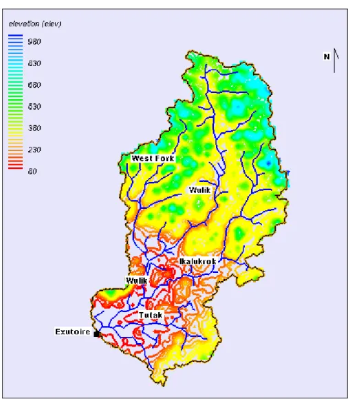
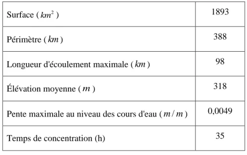
L’algorithme GD-MAT a été appliqué à trois sites de pergélisol afin d’évaluer ses performances avant de l’incorporer dans l’approche PHA. Les trois sites de validation de GD-MAT ont été sélectionnés à partir des études de cas évaluées par Woo et al. (2004), notamment, le site ‘Black Spruce’, le site ‘Aspen Forest’ et le site ‘White Pine’. L’approche PHA a été testée sur le bassin versant Wulik-amont, situé dans la zone de pergélisol continu de l’Alaska. Le bassin versant Wulik-amont est d’une superficie de 1893 km2 caractérisé par un écoulement de surface important de 81% et une infiltration limitée à 15% environ des précipitations.
L’algorithme GD-MAT fournit des résultats de qualité moyenne dans le cas d’un sol de faible teneur en eau. En effet, l’erreur relative sur le domaine temps-profondeurs du gel/dégel simulé du site de ‘White Pine’ caractérisé par une teneur en eau maximale de 0,089 m3/m3 est de 49%. Toutefois, il tend à surestimer la profondeur maximale du gel du sol. L’approche PHA est à même d’effectuer une modélisation hydrologique en prenant en considération la variation de la profondeur du gel/dégel de la couche active, tout en consommant un temps de calcul relativement raisonnable. En effet, le temps de calcul consommé par une simulation du comportement hydrologique du bassin versant Wulik-amont pour la période s’étendant du 26 mai au 23 Septembre 2013 est de 21 minutes. Le maillage généré pour la zone d’étude est uniformément distribué avec une taille de cellule de 500 m x 500 m. La simulation est lancée sur une machine possédant deux processeurs de type Intel(R) Xeon(R) E5-2602 de vitesse de 2,00 GHz.
ABSTRACT
Rising air temperature accompanying climate change will lead to permafrost degradation. Accordingly, the thickness of the active layer will increase. Soil active layer represents an area where major components of the hydrological processes such as evaporation, infiltration and hypodermic flow occur. The active layer undergoes a freeze-thaw sequence through the seasons. During the frost season, it behaves like an impermeable soil layer. However, during the summer season, it becomes a storage for infiltrating water. Depending on the degree of degradation of the permafrost zone, the variation of thawing/freezing depth of the active layer influences the drainage patterns in the watershed. Hence, it is important to take into account the presence of the active layer in the hydrological modeling of a permafrost zone. Some common hydrological modeling systems such as Mike-SHE (Bosson et al., 2013) or GSSHA (Downer and Ogden, 2006) have implemented different approaches to integrate the thickness of the active layer in the assessment of the water balance of a watershed located in a permafrost zone. The major difficulties of the hydrological modeling of a permafrost zone are: the presence of water and heat exchange between the component of soil, the existence of water phase change in the soil layers, the spatial and temporal variation of soil properties and effects of snow cover and vegetation on permafrost warming. Furthermore, information on water content and soil temperature are usually available only locally, hampering hydrological modeling permafrost basins characterized by a large area. Finally, there is a luck of common hydrological models that allows performing a detailed modeling of permafrost behavior.
The main objective of this project is to develop a hydrological modeling tool that reduces significantly the simulation time of the hydrological behavior modeling of permafrost areas. To achieve the overall objective of the project, a characterization of the hydrological behavior of permafrost areas is conducted. Then, an analysis of the modeling approaches used to simulate the spatiotemporal evolution of the active layer freezing and thawing was performed. Moreover, the methods previously used to integrate the freezing and thawing depths of the active layer in the assessment of the water balance of watersheds located in permafrost zone have been described. Furthermore, a permafrost module entitled GD-MAT (Gel Degel-Matlab) is developed on the basis of the unidirectional algorithm Stefan (Woo et al., 2004). This algorithm provides an estimation of the variation of the water/ice content of the ground depending on the depth and
according to the progress of the freezing / thawing front. This ability helps to overcome the lack of measured water content availability at different soil depths which is necessary to Stefan algorithm. GD-MAT is related to GSSHA, physically based distributed model of hydrological modeling, through the maximum capacity parameter of the conceptual groundwater model used for modeling the base flows and the saturated hydraulic conductivity of the soil. The resulting tool from this linkage is called PHA (Permafrost Hydrological Analysis). This is a convenient method for linking a common hydrological model to a model of freezing / thawing of the soil which helps to reduce the computing time consumed by a hydrological modeling of permafrost zone.GD-MAT is linked to the distributed GSSHA model of the hydrological modeling through the maximum capacity parameter of the conceptual groundwater model used for modeling the base flows.
GD-MAT module was applied to three permafrost sites. The three GD-MAT validation sites were selected on the basis of case studies evaluated by Woo et al. (2004), in particular, the site 'Black Spruce', the site Aspen Forest 'and the site' White Pine’. The PHA tool was tested on an upstream watershed of Wulik located in the continuous permafrost zone of Alaska. This watershed with an area of 1893 km2 is mainly characterized by a high runoff coefficient and limited infiltration. The GD-MAT algorithm provides medium-quality results in the case of soil characterized by low humidity. Indeed, the relative error on time-depth domain of simulated freezing/thawing fronts of 'White Pine' site which is characterized by a maximum water content of 0.089 m3/m3 is 49%. However, it tends to overestimate the maximum depth of soil freezing. The PHA approach is able to perform a hydrological modeling taking into account the variation of the depth of freezing / thawing of the active layer while consuming a relatively reasonable computation time. Indeed the computation time consumed by a hydrological simulation of the Wulik river upstream watershed for the period extending from May 26 to September 23, 2013 is 21 minutes. The mesh generated for the study area is uniformly square type, the cell size is 500 m by 500 m. The simulation is launched on a device with two Intel-based processors (R) Xeon (R) E5-2602 speed of 2.00 GHz.
TABLE DES MATIÈRES
DÉDICACE ... III REMERCIEMENTS ... IV RÉSUMÉ ... V ABSTRACT ... VII TABLE DES MATIÈRES ... IX LISTE DES TABLEAUX ... XIII LISTE DES FIGURES ... XV LISTE DES SIGLES ET ABREVIATIONS ... XIX LISTE DES ANNEXES ... XXI
CHAPITRE 1 INTRODUCTION ... 1
1.1 Mise en contexte et problématique ... 1
1.2 Objectifs de la recherche ... 2
1.2.1 Objectifs spécifiques : ... 2
1.2.2 Hypothèses scientifiques ... 2
1.3 Organisation du rapport ... 3
CHAPITRE 2 ARTICLE 1 : HYDROLOGICAL MODELING OF PERMAFROST AREAS: CRITICAL REVIEW OF LITTERATURE AND PERSPECTIVES ... 5
2.1 Introduction ... 5
2.2 Characteristics of permafrost hydrology ... 7
2.3 Hydrological modeling of permafrost areas ... 10
2.3.1 Hydrological models linked to permafrost models in a coupled approach ... 10
2.3.2 Hydrological models linked to permafrost models in a decoupled approach ... 14
2.4.1 Main approximate analytical models ... 22
2.4.2 Selection criteria for a permafrost model ... 26
2.5 Conclusion ... 31
CHAPITRE 3 MÉTHODOLOGIE ET PRÉSENTATION DE L’ALGORITHME GD-MAT, DU MODÈLE HYDROLOGIQUE GSSHA ET DE L’APPROCHE PHA ... 32
3.1 Introduction ... 32
3.2 Description de l’algorithme de Stefan ... 33
3.3 Développement de l’algorithme GD-MAT ... 36
3.4 Description du modèle GSSHA (Gridded Surface Subsurface hydrologic Analysis ) .. 43
3.4.1 Généralités ... 43
3.4.2 Simulation en continu à l’aide du GSSHA 6.1 ... 47
3.4.3 Modélisation hydrologique à l’aide du GSSHA 6.1 ... 56
3.4.4 Description de l’interface WMS ( Watershed Modeling System) ... 57
3.5 Développement de l’approche PHA proposée pour la modélisation hydrologique des zones de pergélisol ... 57
3.6 Conclusion ... 63
CHAPITRE 4 VALIDATION DE L’ALGORITHME PROPOSÉ GD-MAT ET DESCRIPTION DU BASSIN VERSANT WULIK-AMONT ... 64
4.1 Introduction ... 64
4.2 Présentation des sites de validation de l’algorithme GD-MAT ... 65
4.3 Modélisation du gel et dégel du sol au niveau des trois sites de validation à l’aide de GD-MAT ... 66
4.4 Présentation du bassin versant amont de la rivière Wulik et des données disponibles .. 76
4.4.1 Caractéristiques générales du bassin versant Wulik-amont ... 76
4.4.3 Topographie et morphologie ... 82
4.4.4 Données d’occupation du sol et de texture du sol ... 85
4.4.5 Climatologie ... 87
4.4.6 Données pluviométriques ... 87
4.4.7 Données hydrométriques ... 93
4.4.8 Données de débits ... 95
4.4.9 Caractéristique du pergélisol au niveau du bassin versant Wulik-amont... 95
4.5 Conclusion ... 99
CHAPITRE 5 APPLICATION DE L’APPROCHE PHA AU BASSIN VERSANT AMONT DE LA RIVIÈRE WULIK ... 100
5.1 Introduction ... 100
5.2 Préparation du modèle hydrologique GSSHA relatif au bassin versant Wulik-amont 100 5.2.1 Choix de la taille des grilles du maillage ... 100
5.2.2 Choix du pas de temps de calcul ... 104
5.2.3 Description des hypothèses de la simulation du comportement hydrologique du bassin versant Wulik-amont à l’aide de GSSHA ... 106
5.2.4 Analyse de sensibilité du coefficient de rugosité du Manning ... 109
5.2.5 Analyse de sensibilité du coefficient de rugosité du terrain Rt ... 111
5.2.6 Analyse de sensibilité de la conductivité hydraulique du sol ... 113
5.2.7 Analyse de sensibilité de l’épaisseur du sol actif (ESA) ... 113
5.2.8 Analyse de sensibilité de la teneur en eau initiale du sol (SM) ... 114
5.2.9 Analyse de sensibilité de la capacité de stockage maximale de la zone d’écoulement rapide du réservoir conceptuel souterrain ... 115
5.3 Calibration du modèle hydrologique du bassin versant Wulik-amont établi à l’aide de GSSHA ... 115
5.3.1 Procédure de calibration ... 115
5.3.2 Résultats de la calibration ... 117
5.4 Validation du modèle hydrologique du bassin versant Wulik-amont établi à l’aide de GSSHA ... 122
5.5 Discussion des résultats de calibration et validation du modèle établi à l’aide du système GSSHA ... 124
5.6 Modélisation hydrologique du bassin versant Wulik-amont à l’aide de l’approche PHA ………..125
5.6.1 Description des hypothèses de modélisation à l’aide de PHA ... 125
5.6.2 Résultats de la simulation de la réponse hydrologique du bassin versant à l’aide de PHA ………..126
5.7 Conclusion ... 133
CHAPITRE 6 CONCLUSIONS ET RECOMMANDATIONS ... 134
6.1 Contributions ... 136
6.1.1 Contributions à la recherche et au développement... 136
6.1.2 Article soumis dans une revue ... 137
6.1.3 Présentation dans une conférence ... 137
6.1.4 Articles publiés dans une revue ... 137
6.2 Recommandation ... 138
RÉFÉRENCES ... 139
LISTE DES TABLEAUX
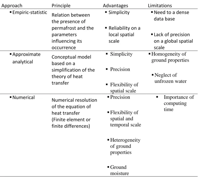
Table 2-1 : Advantages and limitations of three families of permafrost models………….... 20 Table 2-2 : Analysis of approximate analytical models for permafrost region……….. 25 Tableau 3-1 : Principaux processus modélisés à l’aide de GSSHA et leurs techniques
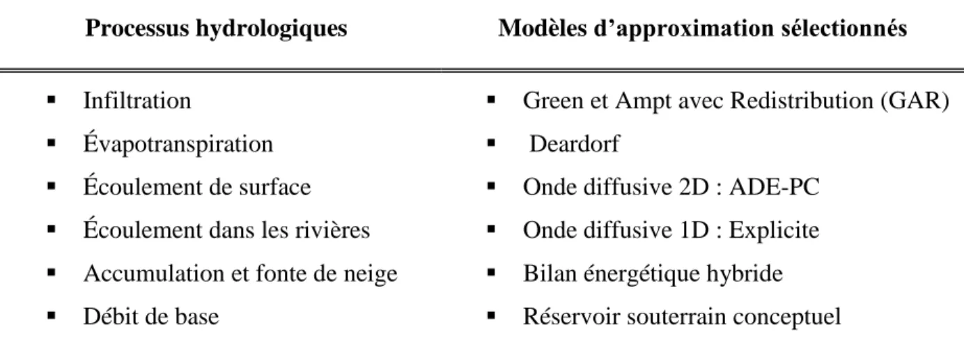
d’approximation ... 44 Tableau 3-2 : Techniques d’approximation des processus sélectionnés pour la modélisation
hydrologique de la zone d’étude ... 48 Tableau 3-3 : Paramètres du modèle du réservoir souterrain conceptuel intégré au sein de
GSSHA6.1 ... 55 Tableau 4-1: Propriétés de sol des sites de validation (adapté de Woo 2004) ... 65 Tableau 4-2: Erreurs relatives sur les temps-profondeurs des trois sites de validation de
l’algorithme GD-MAT ... 69 Tableau 4-3: Dates de début du gel/dégel des trois sites de validation ... 70 Tableau 4-4: Récapitulatif des données collectées sur le bassin Wulik-amont ... 79 Tableau 4-5: Caractéristiques physiographiques du bassin versant amont Wulik éstimées à l'aide
de l'outil WMS 9.1 ... 85 Tableau 5-1 : Étude de convergence du maillage proposé pour la simulation hydrologique du
bassin versant Wulik-amont ... 102 Tableau 5-2: Valeurs des paramètres des modèles d'infiltration, d'évaporation et d'écoulement en
surface sélectionnées pour la simulation hydrologique de base du bassin versant Wulik-amont ... 108 Tableau 5-3: Valeurs des paramètres du modèle du réservoir souterrain conceptuel ... 109 Tableau 5-4: Influence de la variation du coefficient de rugosité de Manning nm sur le volume de
ruissellement calculé, sur le NSE et sur le débit maximal de la période de simulation ... 110 Tableau 5-5: Influence de la variation de la rugosité du terrain Rt sur le volume de ruissellement
Tableau 5-6: Influence de la variation de la conductivité hydraulique Ks des tourbes sur les
volumes d’eau infiltrée et ruisselée calculés à l’aide de GSSHA, sur le NSE et sur le débit maximal de la période de simulation ... 113 Tableau 5-7 : Influence de la variation de l’ESA sur l’estimation des volumes d’eau évaporée
indirectement et drainée vers la zone saturée à l’aide de GSSHA ... 114 Tableau 5-8: Influence de la variation de la teneur en eau initiale des tourbes sur l’estimation des
volumes d’eau évaporée indirectement, ruisselée et drainée vers la zone saturée à l’aide de GSSHA ... 114 Tableau 5-9: Analyse de sensibilité du paramètre FAST_MAX ... 115 Tableau 5-10: Bilan total de masse des composantes hydrologiques de surface relatif à la période
de calibration ... 117 Tableau 5-11: Bilan total de masse de l'humidité du sol relatif à la période de calibration... 118 Tableau 5-12: Résultats des indicateurs de performance de l'étape de calibration du modèle
GSSHA ... 120 Tableau 5-13: Valeurs des paramètres hydrologique retenues après l’étape de calibration ... 122 Tableau 5-14: Bilan total de masse des composantes hydrologiques de surface relatif à la période
validation ... 122 Tableau 5-15: Bilan total de masse de l'humidité du sol relatif à la période de validation ... 123 Tableau 5-16: Résultats des indicateurs de performance de l'étape de validation du modèle
GSSHA ... 124 Tableau 5-17 : Propriétés des couches de sol utilisées pour la modélisation du gel/dégel de la
couche active du bassin versant Wulik-amont ... 126 Tableau 5-18: Volume d'eau infiltrée et ruisselée estimés pour les deux simulations, avec et sans
pergélisol, sur la période de 26 mai au 23 juillet ... 129 Tableau 6-1: Avantages et limites de l'approche PHA ... 136
LISTE DES FIGURES
Figure 2.1 : Proposal schema for selecting a permafrost model ... 30
Figure 3.1: Algorithme GD-MAT de calcul de l’avancement du gel/dégel du sol ou de la couche active ... 40
Figure 3.2 : Procédure de calcul du gel ... 41
Figure 3.3 : Procédure de calcul du dégel ... 42
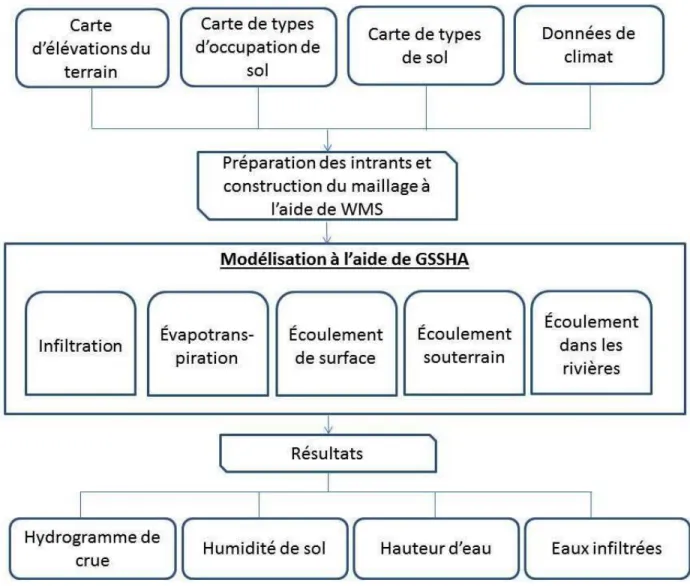
Figure 3.4 : Étapes nécessaires à une simulation hydrologique à l’aide de GSSHA 6.1 ... 46
Figure 3.5 : Avancement du front d'humectation dans le sol modélisé à l'aide de GAR pendant la redistribution des eaux infiltrées (Ogden and Saghafian, 1997) ... 49
Figure 3.6 : Schéma explicite associé à la modélisation de l'écoulement dans les cours d'eau (Downer and Ogden, 2006) ... 51
Figure 3.7 : Schéma du modèle du réservoir souterrain conceptuel (Follum and Downer, 2014) 54 Figure 3.8 : Intrants et sorties de l'approche PHA proposée pour la modélisation hydrologique des zones de pergélisol ... 59
Figure 3.9 : Organigramme de l’approche PHA ... 60
Figure 4.1: Comparaison des fronts de gel et dégel simulés et observés au niveau du site ‘Black Spruce Forest’. ... 67
Figure 4.2: Comparaison des fronts de gel et dégel simulés et observés au niveau du site des ‘White Pine’ ... 68
Figure 4.3: Comparaison des fronts de gel et dégel simulés et observés au niveau du site de ‘Aspen Forest’ ... 69
Figure 4.4: Teneurs en glace (à droite) et en eau (à gauche) du sol estimées à l'aide de GD-MAT aux profondeurs suivantes : 5 cm (ligne bleue), 35 cm (ligne verte) et 65 cm (ligne rouge). a) désigne le site ‘Black Spruce Forest’, b) est le site ‘White Pine’ et c) représente le site ‘Aspen Forest’ ... 71
Figure 4.6: Position de la ligne isotherme 0°C du site boréal d'‘Black Spruce Forest’. La partie supérieure de la figure montre les températures de sol (T) à différentes profondeurs ... 74 Figure 4.7: Profils de température dans le sol durant les journées de 24 et 28 décembre 1999 du
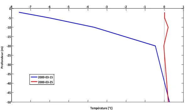
site boréal d'‘Black Spruce Forest’ ... 75 Figure 4.8: Profil de température dans le sol durant les journées de 15 et 25 mars 2000 du site
boréal d'‘Black Spruce Forest’ ... 75 Figure 4.9: Fronts de gel/dégel observés (point) et évalués (ligne) à l'aide de l'algorithme
bidirectionnel de Stefan au niveau du site ‘Black Spruce Forest’sur la période de septembre 1999 au mois d’août 2000. ( Adapté de Woo et al., 2004)... 76 Figure 4.10: Situation géographique du bassin Wulik-amont, carte élaborée à l’aide de WMS. .. 77 Figure 4.11 : Vue du bassin versant Wulik-amont (Adaptée à partir de Google Earth 2015) ... 80 Figure 4.12: À gauche, une vue de la rivière Wulik durant juin ... 81 Figure 4.13: La fonte du pergélisol et la fonte des lentilles de glace ajoutent la turbidité de la
rivière Wulik (Adaptée de Permafrost Dynamics and Soil Carbon, V.Romanovsky, 2007) . 81 Figure 4.14:Vue aérienne de site de jaugeage sur la rive gauche de la rivière Wulik, du cotée de la
branche Tutak près de Kivalina, Alaska le 7 Juin 2001 (Adaptée de (USGS, 2005)) ... 82 Figure 4.15:Altitudes du bassin versant Wulik-amont (en mètres), carte élaborée à l’aide de WMS ... 83 Figure 4.16 : Physiographie du bassin versant Wulik-amont (Adaptée, Alaska division of
geological and geophysical survey, 1982-1983) ... 84 Figure 4.17: Principaux types de sol du bassin amont de la rivière Wulik ... 86 Figure 4.18: Normales de température à la station de météo Kivalina sur la période 1980-2010 . 87 Figure 4.19: Équipement hydro-météorologique au niveau du bassin versant amont de la rivière
Wulik ... 88 Figure 4.20: Localisation des stations météorologiques utilisées lors du traitement des données de
Figure 4.21: Comparaison des précipitations mensuelles de la station Red Dog Mine de 2010 à 2014 avec les normales mensuelles de précipitations au niveau de la station Kotzebue Wso Ap ... 90 Figure 4.22: Comparaison des précipitations mensuelles de la station Kivalina Airport de 2011 à
2014 avec les normales mensuelles de précipitations au niveau de la station Kotzebue ... 92 Figure 4.23: Comparaison des températures mensuelles de la période 2010-2013 avec les
normales mensuelles de la station Kotzebue ... 94 Figure 4.24: Profil de sol au niveau du site Ikalukrok (Adapté à partir de (USDA, 2012)) ... 96 Figure 4.25: Teneurs en eau mesurées du sol de l'année 2011 à différentes profondeur au niveau
du site Ikalukrok (http://www.wcc.nrcs.usda.gov/nwcc/view) ... 96 Figure 4.26:Températures mesurées du sol de l'année 2011 à différentes profondeur au niveau du
site Ikalukrok (http://www.wcc.nrcs.usda.gov/nwcc/view ) ... 97 Figure 4.27: Comparaison de la variation des températures mesurées de l'air et celles du sol à une
profondeur de 5,08 cm (http://www.wcc.nrcs.usda.gov/nwcc/view ) ... 98 Figure 5.1:Hydrogrammes de crue calculés à l'aide de GSSHA en utilisant les maillages 1000m,
800m, 500m et 250m ... 103 Figure 5.2: Étude de convergence temporelle du modèle hydrologique du bassin versant Wulik-amont établi à l'aide de GSSHA ... 105 Figure 5.3 : Hydrogrammes de crue correspondant aux pas de temps 10s, 60s, 100s et 180s .... 106 Figure 5.4: Débits calculés selon des coefficients de rugosité de Manning (nm) distincts à l'aide de
GSSHA au niveau de l'exutoire de la zone d'étude pour la période du 13-08-2012 au 30-08-2012 ... 111 Figure 5.5:Débits calculés selon des coefficients de rugosité de terrain (Rt) distincts à l'aide de
GSSHA au niveau de l'exutoire de la zone d'étude pour la période du 13-08-2012 au 30-08-2012 ... 112 Figure 5.6: Hydrogramme de crues du bassin versant Wulik-Amont résultant de la calibration du
Figure 5.7:Hydrogramme de crues du bassin versant Wulik-Amont résultant de la calibration du
système GSSHA, juillet 2011- octobre 2011 ... 119
Figure 5.8:Hydrogramme de crues du bassin versant Wulik-Amont résultant de la calibration du système GSSHA, décembre 2012- octobre 2012 ... 119
Figure 5.9:Hydrogramme de crues du bassin versant Wulik-Amont résultant de la calibration du système GSSHA, août 2012 ... 120
Figure 5.10: Résultats de la validation du modèle calibré à l'aide du système GSSHA ... 123
Figure 5.11: Profondeurs de gel/dégel estimées à l'aide de PHA, Wulik-amont ... 127
Figure 5.12: Hydrogrammes évalués avec et sans pergélisol, Wulik-amont ... 128
Figure 5.13: Hydrogrammes évalués avec et sans pergélisol pour la période s’étendant du 27 mai au 28 juillet 2013 ... 128
Figure 5.14: Variation de la conductivité hydraulique à saturation du sol estimée à l'aide de PHA ... 130
Figure 5.15: FAST_MAX calculé à l'aide de PHA sur la période de mai à octobre 2013 ... 130
Figure 5.16: Teneurs en eau simulés du sol (lignes discontinues) à l’aide de l’algorithme GD-MAT incorporé au niveau de l’approche PHA, teneurs en eau observées du sol (ligne continue), Wulik-amont ... 131
LISTE DES SIGLES ET ABREVIATIONS
ACRC Alaska Climate Research Centre
ADE Alternating Direction Explicit
ADE-PC Alternating Direction Explicit with Prediction Correction ASCII American Standard Code for Information Interchange
CFGI Continous Frozen Ground Index
CLM Common Land Model
CPU Central Processing Unit
CRHM Cold Region Hydrologic Model
DEM Digital Elevation Map
EnvM Environmental Module
ERDC U.S. Army Engineer Research and Development Center
ESA Épaisseur du Sol Actif
ETA Évapotranspiration Actuelle
ETP Évapotranspiration Potentielle
FAST_MAX
Capacité de stockage maximal de la zone d'écoulement rapide du réservoir souterrain (mm)
GAR Green and Ampt with Redistribution
GD-MAT Gel Dégel-Matlab
GIEC Groupe Intergouvernemental sur l'Évolution de Climat GIPL Geophysical Institute Permafrost Laboratory
GSSHA Gridded Surface Subsurface Hydrological Analysis HBV Hydrologiska Byråns Vattenbalansavdelning
HEC-HMS Hydrologic Engineering Center- Hydrologic Modeling System
HRU Homogeneous Hydrological response Unit
LLNL Lawrence Livermore National Laboratory
MAAT Mean Annual Air Temperature
NOAA National Oceanic and Atmospheric Administration NRCS Natural Resources Conservation Service
PHA Permafrost Hydrological Analysis
RE Richards Equation
RMSE Root Mean Square Error
SAC-SMA Sacramento Soil Moisture Accounting
SCE Shuffled Complex Evolution
SHAW Simultaneous Heat And Water
SLOW_MAX
Capacité de stockage maximal de la zone d'écoulement rapide du réservoir souterrain (mm)
TEM Terrestrial Ecosystem Model
TTOP Temperature at The Top Of Perennial frozen/unfrozen soil
U.S. United States
USDA United State Departement of Agriculture
USGS United State Geological Survey
UZFWM Upper zone free water capacity
LISTE DES ANNEXES
ANNEXE A VÉRIFICATION DE LA VALIDITÉ DE L’ÉQUATION DE
CHAPITRE 1
INTRODUCTION
1.1 Mise en contexte et problématique
Le pergélisol occupe environ un quart de la surface du globe et couvre 22% des terres de l’hémisphère nord. Il correspond aux sols maintenus à une température inférieure à 0°C pendant deux années consécutives au moins (Dolnicki et al., 2013). Selon le rapport du Groupe d’Experts Intergouvernemental sur l’Évolution du Climat (GIEC, 2007) le réchauffement prévu du 21ème siècle (~ 5°C) sera suffisant pour initier la dégradation du pergélisol dans de nombreuses régions nord-américaines. Par conséquent, l’augmentation de la profondeur du gel/dégel de la couche active influencera le régime d’écoulement des bassins versants situés dans une zone de pergélisol. D’où la nécessité d’adapter les modèles hydrologiques actuels afin de mieux caractériser le comportement hydrologique de ces zones. Pour ce faire, il s’avère intéressant de développer un module de calcul fiable de l’épaisseur de la couche active, représentant la profondeur du gel/dégel, qui devra être intégrée dans le modèle hydrologique approprié pour les régions de climat froid.
Étant donné que la dynamique du pergélisol est gouvernée par l’échange de flux de chaleur et d’eau entre ses différentes couches, l’évaluation des débits d’eau à l’exutoire des bassins versants consiste à résoudre simultanément les équations du bilan hydrique et du bilan d’énergie au niveau du pergélisol (Li et al., 2010; Lunardini, 1981; Xia, 1993). Pour ce faire, certains auteurs ont couplé un modèle hydrologique à un modèle de pergélisol. En effet, le module de pergélisol calcule la profondeur du gel/dégel; et celle-ci est renvoyée au modèle hydrologique afin qu’elle soit introduite dans l’équation du bilan hydrique (Hinzman and Kane, 1992; Xia, 1993).
La difficulté de la modélisation hydrologique du pergélisol réside dans la présence de changement de phase de l’eau, la variation spatio-temporelle des propriétés du sol et les effets du couvert de neige et de végétation sur le réchauffement du pergélisol (Lunardini, 1981; Woo, 2012). Dans ce sens, des méthodes de résolution numériques ont été utilisées pour déterminer la profondeur du gel/dégel (Hinzman et al., 1998; Marchenko et al., 2008). Bien que les méthodes numériques aboutissent à des résultats satisfaisants, elles sont coûteuses en temps de calcul et elles nécessitent de puissantes machines. Afin de remédier à l’utilisation des modèles numériques dans certaines conditions, des formules empiriques basées sur des corrélations entre la
température de l’air, les propriétés du sol et la profondeur de pergélisol ainsi que des approches analytiques approximatives fondées sur la simplification du problème d’échange de flux de chaleur et d’eau dans le sol pourraient être utilisées (Riseborough et al., 2008). Les méthodes empiriques nécessitent une base de données dense et ne peuvent généralement être appliquées qu’à l’échelle locale. Par contre, les approches analytiques approximatives sont caractérisées par leur simplicité. De plus, elles sont valides à l’échelle locale et régionale (Riseborough et al., 2008). Ainsi, coupler un modèle hydrologique à un modèle de calcul de l’épaisseur de la couche active basé sur une approche empirique ou analytique approximative constitue une bonne alternative. En effet, cela permet aussi bien de réduire le temps de simulation que prendre en compte la variation de certaines propriétés du sol telle que l’humidité.
1.2 Objectifs de la recherche
L’objectif général du présent travail de recherche est de développer un outil de modélisation hydrologique des régions nordiques qui intègre la dynamique du pergélisol et qui soit rapide en terme de temps de calcul.
1.2.1 Objectifs spécifiques :
1- Identifier les caractéristiques hydrologiques des zones de pergélisol
2- Établir les critères de choix d’un modèle de simulation du gel/dégel du sol.
3- Développer une approche de modélisation hydrologique adaptée aux zones de pergélisol
1.2.2 Hypothèses scientifiques
Hypothèse 1 : Le choix judicieux d’un modèle de pergélisol optimise les moyens nécessaires au
calcul du gel/dégel du sol et améliore la recherche des résultats souhaités.
Originalité: jusqu’à présent, il n’existe pas de critères de choix d’un modèle de pergélisol
(Bonnaventure and Lamoureux, 2013; Riseborough et al., 2008)
Réfutabilité : l’hypothèse sera réfutée si les critères ne sont pas aussi défendables pour
qu’elles soient publiées dans un journal scientifique.
Hypothèse 2 : L’équation de Stefan permet de réduire le temps de simulation du gel/dégel du
Originalité: l’application de l’équation de Stefan dans le calcul de la profondeur du
gel/dégel du sol n’a pas fait l'objet d’une étude hydrologique antérieure à l’échelle d’un bassin versant situé dans une zones de pergélisol (Marchenko et al., 2008; Sazonova and Romanovsky, 2003).
Réfutabilité : l’hypothèse sera réfutée si le temps de calcul dépasse deux jours et demi.
Cette limite est mise en place en se référant aux deux études de cas de modélisation hydrologiques effectuées pour les bassins versants appelés ‘Little Washita’ et ‘Central Oklahoma’. Dans le premier cas, la simulation hydrologique a duré deux jours et demi et pour le deuxième, quatre jours environ (Maxwell et al., 2006).
Hypothèse 3 : Un modèle hydrologique simulant l’écoulement des eaux de surface et
souterraines ainsi que les échanges en eau entre les deux domaines, couplé à un modèle de pergélisol basé sur une méthode analytique approximative, prend en compte la variation de la profondeur du gel/dégel de la couche active dans l’évaluation de la contribution des eaux souterraines dans les débits des cours d’eau.
Réfutabilité: l’hypothèse sera réfutée si la forme de l’hydrogramme et les débits de pointe
évalués à l’aide de cette approche sont similaires à ceux estimés, en négligeant la présence de la couche active.
1.3 Organisation du rapport
Le présent mémoire est composé de six chapitres, à savoir :
Le chapitre 1 met dans un premier temps en contexte la problématique de la dynamique du pergélisol, ensuite il présente l’objectif général du travail de la recherche, les objectifs spécifiques et les hypothèses scientifiques effectuées pour la réalisation du présent projet.
Le chapitre 2 est une revue critique de la littérature portant sur la modélisation hydrologique des zones de pergélisol. Cette revue bibliographique comporte trois parties : la première présente l’hydrologie des zones de pergélisol, la deuxième décrit les outils et les approches de modélisation hydrologique employés pour la simulation de la réponse des zones de pergélisol, et la troisième présente les approches utilisées pour la modélisation du gel/dégel du sol, en particulier de la couche active.
Le chapitre 3 comprend une description de la méthodologie du travail ainsi qu’une présentation des outils de modélisation sélectionnés lors du présent projet. Il présente également l’approche proposée pour atteindre l’objectif général de la recherche.
Le chapitre 4 consiste en une justification de l’utilisation de trois études de cas traitées dans la présente recherche ainsi que les résultats de validation de l’algorithme GD-MAT.
Le chapitre 5 présente la préparation, la calibration et la validation du modèle hydrologique de la zone d’étude préparé à l’aide de GSSHA 6.1. Il présente également les résultats de l’application de l’approche proposée pour intégrer la variation de l’épaisseur de la couche active au niveau du calcul du bilan hydrique de la zone d’étude.
Le chapitre 6 présente une discussion générale et une conclusion mettant en évidence les limites de l’approche proposée et suggérant des recommandations.
CHAPITRE 2
ARTICLE 1 : HYDROLOGICAL MODELING OF
PERMAFROST AREAS: CRITICAL REVIEW OF LITTERATURE AND
PERSPECTIVES
Abstract
Climate change will have a significant impact on the hydrology of cold regions due to the dynamic of the permafrost layer that comes with these changes. Modeling adequately these dynamics becomes more and more a great concern. Hydrological modeling of permafrost has seen an outstanding progress since the end of the 20th century. Progress still remains to be made in this direction to improve the computation time while preserving an acceptable level of accuracy. The present paper provides a critical analysis of the most used permafrost modeling approaches and models developed for the simulation of hydrological processes in permafrost areas. A series of selection criteria is suggested as a support tool in the process of choosing a proper permafrost model. The analysis of existing models shows that linking a hydrological model to a permafrost model in a coupled approach leads to a more accurate representation of permafrost hydrology.
Key words: Permafrost, hydrological modeling, active layer
2.1 Introduction
Permafrost is the type of soil maintained at a temperature below 0 ° C for at least two consecutive years (Dolnicki et al., 2013). It occupies about one quarter of the globe (Anisimov and Nelson, 1996; Nelson et al., 2002). Permafrost covers 22% of the land at the northern hemisphere (Woo, 2012). It is present in cold climate regions including Arctic, Antarctic, and in some mountain areas. A permafrost zone mainly consists of three layers. The upper part is the active layer. It undergoes a seasonal freeze-thaw according to temperature variations. Below lies the horizon of permafrost which is permanently frozen. Finally, the base is formed by a soil layer which does not undergo freezing, despite the low or negative temperatures that can be reached. The characteristics of permafrost, especially the active layer thickness, vary with climate conditions. Based on the spatial continuity of the permafrost horizon, two main types of permafrost area are
distinguished: the continuous and discontinuous permafrost. The continuous permafrost accounts for 90% of permafrost (Woo, 2012). The IPCC report (Stocker et al., 2013) asserts that towards the end of this century, the decrease in the extent of permafrost areas may reach 81%. Consequently, the hydrology of cold climate regions would be affected by this change (Schaefer et al., 2012). Indeed, permafrost degradation leads to an increase in the thickness of the active layer where major hydrological processes occur. Thus, it is important to take into account the presence of permafrost in a hydrological modeling. The variation of active layer thickness through seasons may either increase or decrease the water flow rate at the outlet. Nevertheless, few usual hydrological models represent in detail the hydrological processes of a watershed located in a permafrost area. They reproduce the conditions characterizing cold climate regions by adjusting some hydrological parameters affecting infiltration and storage capacity of the watershed. For example, the hydrological model GSSHA (Gridded Surface Subsurface Hydrologic Analysis) takes into account only the presence of frozen soil by calculating a parameter which depends on the air temperature and indicates whether the active layer is in a state of freezing or thawing in order to properly estimate the infiltration. However, in permafrost zone, the active layer acts as an impermeable layer during the winter season, but becomes a water storage tank in the summer (Hinzman and Kane, 1992; Woo, 2012; Woo, 1986; Yi et al., 2009). An appropriate hydrologic modeling consists of simultaneously solving heat transfer and migration of moisture in the soil equations. Many couplings of hydrological models to permafrost models have been made to consider the permafrost in the calculation of the water balance of a watershed (Flerchinger, 2000; Fox, 1992; Hinzman et al., 1998; Hinzman and Kane, 1992; Yi et al., 2009). However, the use of a permafrost model based on the numerical resolution of the conduction equation requires significant computation time and powerful computing machines especially if it demands a high degree of accuracy of results through a fine discretization of the soil column (Mölders and Romanovsky, 2006). Indeed, in a study of hydrological modeling of the watershed on the Kuparuk river, where the hydrological model HBV was linked to a permafrost model solving conduction equation by the finite element method , Hinzman et al (1998) used 64 parallel processors on the ARSC Cray T3D for a simulation period of 109 days with 1 day time step and 26656 nodes on 1 km spacing. Another example of the heaviness of computation time of numerical modeling is hilighted through the 3D modeling of surface and subsurface water exchanges at the Little Washita watershed and Central Oklahoma
performed by Maxwell et al. (2006). In this study the groundwater ParFlow model was coupled with the landsurface model CLM as a single column model. the Central Oklahoma watershed was represented with 128x88 surface nodes at 1km resolution and 40 vertical cells at 0,5 m resolution. The Little Washita catchment was represented with 128x88 surface nodes at 350 m resolution and 392 vertical cells at 0,5 m resolution. The central Oklahoma simulation takes about 60 hours to run one year at hourly time steps using 32 processors of Intel Xeon 3,02Ghz CPU type. However, the Little Washita hydrological modeling was run on 170 processors of a LLNL institutional machine (2.6GHz) and took about 100 hours to simulate one year at hourly time steps (Maxwell et al., 2006). Furthermore, the calculation time increases extremely when using a distributed hydrological model employing mesh representation of the study area applied at a large scale (Bowling et al., 2008).
Thus, the challenge of permafrost hydrological modeling is to develop a compromise between the accuracy of the simulation of the hydrological behavior of permafrost and the time consumed by the model, so that it can be used on usual calculation machines.
The present paper is a critical review of the progress of freeze / thaw modeling and hydrological modeling of permafrost. In order to achieve this goal , an analysis of the characteristics of permafrost hydrology is carried out in a first step. Then a critical review of hydrological modeling approaches developed for the simulation of permafrost areas is provided. Finally, the families of models used for permafrost modeling are presented with the advantages and disadvantages of each one. A particular emphasis is made on the approximate analytical models and a set of criteria is proposed to guide in the process of selecting an adapted permafrost model.
2.2 Characteristics of permafrost hydrology
The hydrology of permafrost regions is essentially characterized by the accumulation of snow on the soil surface and the formation of ice in the ground. Consequently, changes in the flow of water and the hydrological behavior of watersheds with cold climate have been observed (Hinzman and Kane, 1992; Lunardini, 1981; Woo, 2012). Indeed, the presence of ice in the pores of soil and ice lenses within the active layer slows the infiltration rate and prevents efficient recharging of deep groundwater. In addition, during thawing season, the active layer constitutes a water storage tank, thereby increasing the water retention capacity (Hinzman and Kane, 1992;
Woo, 1986). Moreover, snow cover contributes to the glaciation of hypodermic water and therefore delays the surface runoff (Woo, 2012).
The development of permafrost and its characteristics such as the active layer thickness, the continuity of permafrost or the presence of ice depend on various factors. Woo (2012) enumerates seven parameters influencing the occurrence of permafrost whith the main ones being the location and topography of the area. Indeed, these two factors influence the climate and therefore permafrost. For example, on coastal areas at the Arctic, marine effect tends to soften the climate preventing the formation of permafrost. Other parameters such as snow cover, vegetation and soil type affect the mechanism of heat transfer in soil and determine the formation of permafrost. During the winter, snow protects the soil against the heat dissipation and delays soil warming in the spring. During the summer, a dense crop canopy shelters the ground from sunlight so that the warming of the soil is moderate. Furthermore, the thermal properties of the ground govern the rate of heat dissipation through the soil. Woo (2012) also mentioned other factors influencing the occurrence of permafrost namely the proximity of wetlands, fires and geothermal activity. The three elements tend to warm permafrost by transmitting large amounts of heat.
The hydrological cycle of permafrost goes through three periods: the freezing period, the period of melting snow, and the summer period (Hinzman et al., 1998; Woo, 2012). The freezing period, which lasts for a period of 6 to 10 months, is characterized by the progressive freezing of the active layer and the accumulation of snow on the surface. Indeed, since the surface temperature is cold, the freezing front advances from the surface to the permafrost table. In addition, a freezing front advances from of the active layer bottom to the surface because of the thermal gradient between the two horizons (Romanovsky and Osterkamp, 1997; Woo, 1986). The freezing front progress depends on four factors which are the snow cover thickness, the soil composition, the soil moisture and the presence of lateral flow. The influence of the first two factors on the progress of freezing front is related to the parameter of thermal conductivity. In the case of low thermal conductivities, snow cover and the upper ground act as a thermal insulator. Furthermore, the presence of water in the soil promotes the development of ice within the active layer. Thus, the temperature of the active layer increases due to the latent heat during the passage from a liquid state to a solid state. Therefore, the progress of the freezing front is slowed. Moreover, the lateral flows bring heat convected from a source nearby, preventing cooling the active layer.
The freeze period is also characterized by the migration of moisture from the wet area of the active layer to the unsaturated zone. Indeed, a hydraulic gradient is created between the two zones due to the formation of ice in the pores of the unsaturated portion where the temperature is 0 ° C (Guymon, 1975; Woo, 2012). Thus, at the end of the winter season, the freezing front progress becomes maximum; the active layer acquires a minimum water content and acts as an impermeable layer (Hinzman and Kane, 1992; Woo, 2012). The spring season characterized by snowmelt is a transition between the two periods of winter and summer. In fact during the spring, the snow stored along the winter on the soil surface is exposed to sunlight for long periods. Therefore, the two processes of sublimation and snowmelt are initiated. Part of the liquid water can infiltrate through the active layer where it refreezes due to a temperature below 0 ° C. Also, basal ice is formed at the interface of snow cover / ground surface derived from the refreezing of snow melt water when in contact with soil surface (Woo, 2012). During this season, the presence of ice at the surface or in the ground reduces infiltration rate of snow melt water (Gray et al., 1985; Gray et al., 2001). Moreover, the change of phase of infiltrated water into ice tends to increase the temperature of the active layer (Zhao and Gray, 1997). Thus, the beginning of the thaw of the active layer coincides with the total disappearance of the snow cover (Woo, 1986). Runoff from snowmelt begins when the infiltration reaches the stage of equilibrium. The end of the spring season is essentially marked by the complete melting of snow cover generating runoff, early thaw of the active layer and the increase of the water content of the active layer. Generally the period of snowmelt extends over a period of a few weeks (Woo, 2012; Woo, 1986).
Finally, the summer season marking the end of the annual hydrological cycle usually occurs in June or July and lasts for a period of about two months (Woo, 2012). Summer is a key stage in water rooting of the cold regions, because the majority of hydrological processes occur during this period (Hinzman and Kane, 1992). First, increasing the temperature of the ground surface allows for the active layer to acquire a large heat flux. Consequently the thawing front advances gradually towards the active layer bottom. The advance of thaw depends mainly on soil properties and its water and ice content (Ming-ko and Zhaojun, 1996; Woo, 1986). At the same time, a part of rainfall water infiltrates into the ground accompanied with a transfer of heat to the ground so that the thawing process is accelerated. Hence the water content of the active layer increases. A second part of the water evaporates through the water surface, bare ground and vegetation (Woo, 2012). Then, surface runoff occurs when the active layer is completely
saturated with water (Woo, 1986). It should be noted that the storage capacity increases with thaw active layer thickness. During the summer season, thawing of the active layer and moisture reach their maximum values.
Thus, the hydrological behavior of permafrost areas is relatively complicated because it is governed not only by water transfer between watershed components, but also by heat transfert wich controlls the snowmelting and freezing-thawing of the active layer. Therfore, hydrological modeling of permafrost areas is mainely based on resolving simultaneousely water balance and energy balance equations.
2.3 Hydrological modeling of permafrost areas
Hydrological modeling constructs a simplified mathematical representation of the real flow of water within a watershed to anticipate its hydrological response. It mainly involves the following components: surface runoff, groundwater flow and water quality (Singh et al., 2002). In regions with cold climate, hydrological modeling of permafrost areas experienced a prominent progress since the 1990s. In fact, the importance of changes in hydrological processes in the presence of permafrost has prompted scientists to integrate the calculation of freezing / thawing of the active layer in the evaluation of the water balance. Hydrological permafrost models are based on different approaches with different complexity degrees. Two approaches have usually been adopted to address the issue of hydrological modeling of permafrost. The first method is decoupled approach in which the determination of freeze / thaw of the active layer is performed separately from the calculations of water balance. In fact, in this case, active layer thickness is introduced as a modeling parameter of the hydrological simulation (Hinzman and Kane, 1992). The second method is called coupled approach which solves simultaneous equations governing heat transfer and water flow through ground components (Flerchinger and Saxton, 1989; Yi et al., 2009).
2.3.1 Hydrological models linked to permafrost models in a coupled approach
The Fox (1992) model)
In 1992, Fox modified the hydrological model HYFOR (Fox, 1976) so that the calculation of active layer thickness is incorporated in the assessment of the water balance. Following a daily
time step, Fox model (1992) simulates the main hydrological processes including: snowmelt, evapotranspiration, infiltration and subsurface flow through a vertical column of soil. Permafrost modeling is performed using an algorithm proposed by Jumukis (1977) as the solution of Stefan problem. Indeed, Jumukis model constitutes the starting point of the bidirectional Stefan-algorithm proposed by Woo (2004). The linkage between the hydrological model and Jumukis’s algorithm (1977) is done in two ways: 1) the effect of soil moisture on the thermal conductivity and the volumetric latent heat of fusion and 2) the effect of the ice content on the infiltration and water migration in the vertical column of soil. After estimating the freeze / thaw of the active layer for each day, an update of the moisture and ice contents is performed at each soil horizon. Then the revaluation of the freeze / thaw of the active layer and the calculation of the water balance of the column are set for the following day. The sensitivity analysis of the model showed that the parameters influencing Fox model (1992) are: snow cover depth and timing, snow cover of the top, air temperature, organic layer thickness and soil properties (Fox, 1992; Xia, 1993). The strength of the Fox model (1992) lies in its ability to couple permafrost modeling in the evaluation of water balance so that the effect of each process on the other will be considered. Nevertheless, the use of the Jumukis’s algorithm (1977) does not allow taking into account the advancement of frost front from active layer bottom to the surface.
SHAW model (Flerchinger, 2000)
The SHAW model (Simultaneous Heat And Water) was developed to model permafrost dynamics (Flerchinger and Saxton, 1989). It is a one-dimensional model allowing the simulation of exchanges of water and heat between the canopy, snow cover, residue and the ground. Also Shaw is able to model the transport of pollutants through a vertical column of soil (Flerchinger, 2000). Operation of SHAW model follows three main steps. At first, the heat transfer and water exchange equations are established for each compartment. They are then simultaneously solved to determine the general temperature profile and the global distribution of moisture in the study domain. For this purpose, the equations describing the heat transfer and water migration are expressed in the implicit finite difference method and solved using the iterative Newton-Raphson approach. Then, infiltrate water is quantified using the Green-and-Ampt method. Finally, an update of the soil temperature and moisture content is carried out to account for the heat and the water introduced by infiltration in ground.
Freezing/thawing soil layer is mainly described by equations (1) and (2) :
2-1
Where is the volumetric fraction of water ( ), the volumetric fraction of ice ( ), and densities of water and ice ( ), the unsaturated hydraulic conductivity ( ), the soil matric potential (m), the vapor flux ( ) and the source term of water (
).
2-2
Where and are volumetric heat capacity ( ) and temperature ( ) of the ground;
f
L and Lf the latent heat of fusion and vaporization (J Kg/ ) respectively; cl the heat capacity
of water (J Kg C/ . ); ksthe thermal conductivity of the ground (W m C ); / . qvand ql vapor flux (
2
/ .
Kg m s) and water flux (m s ); and /
v is vapor density (Kg m/ 3).Equation (1) expresses the variation of ice and water content based on water and vapor quantities available in the soil layer and the water source term which can be sometimes extracted with roots (Flerchinger, 2000).
Equation (2) describes the energy balance of the soil layer associated with a phase change. Indeed, going from the left to the right, the second term represents the latent heat required for water freezing, and then the heat flow transported by conduction and convection are described respectively by the fourth and the fifth term of the equation. Finally, the last term reflects the latent heat required for evaporation of water in the soil layer. The performance of SHAW model in simulating the exchanges of water and energy through a vertical column of soil was demonstrated in several studies (Li et al., 2013). In fact, the use of simultaneous simulation of water exchanges and heat transfers gives a better approximation of the hydrological behavior of the active layer. In addition, the SHAW model accurately treats the variety of vegetation type and its impact on the hydrology of the studied area. However, Shaw is a Soil-Vegetation-Atmosphere (SVAT) model which does not integrate an essential part of the water path namely the generation
1 1 l i i v l l q k U t t z z z l 3 3 m m i m m3 3 l i 3 / kg m k m s/ qv kg m s/ 2. U 3 3 / . m m s i l v v s i f s l l v q T q T T C L k c L t t z z z z t s C T 3 / . J m C C
of surface runoff. Thus, the use of this model to perform a modeling of the hydrological behavior of a watershed located in the permafrost zone requires a linkage of SHAW to a usual hydrological model.
TEM model (Terrestrial Ecosystem Model 2009)
TEM model describes dynamics governing carbon and nitrogen through the terrestrial ecosystem components, including air, soil and vegetation (Raich et al., 1991; Yi et al., 2009; Yi et al., 2014). In order to integrate hydrological processes and heat exchange in the TEM model, Yi et al (2009) developed a module called EnvM (Environmental module) for hydrological simulation of permafrost by considering the active layer freeze / thaw in the evaluation of water balance. The bidirectional Stefan algorithm (Woo et al., 2004) was used to determine the progress of frost front within the active layer. In addition, the N-factor method (Riseborough et al., 2008) was used to estimate the temperature of the ground surface or the snow cover surface from the air temperature. The consideration of active layer freeze / thawing in the water balance is ensured by three points: 1) the runoff evaluation taking into account the position of the hydrostatic level of the groundwater; 2) the determination of the base flow by considering the state of freeze / thaw of the underground soil layers; and 3) the regular updating of moisture. The sensitivity analysis of EnvM demonstrated that the major parameters influencing the model are: the air temperature during summer season, the organic layer thickness and the minimum thermal conductivity of the ground. The strength of this module is the fact that parameters determining the freezing / thawing of the active layer, including soil moisture, are updated at each time step before applying the Stefan-algorithm. Hence, the dynamics of soil moisture in the active layer is better represented. However, the use of Richard's equation to describe the movement of water in the soil and the numerical resolution by finite difference of heat transfer equation requires a large computation time and would need the use of powerful computing machines. Although TEM is not a hydrological model, it was deemed interesting to present it to demonstrate the effectiveness of the Stefan solution to model the spatiotemporal evolution of the thickness of the active layer and adequately represent exchanges flux of heat and moisture in the soil components.
GSSHA model coupling to GIPL2 model (2013)
GSSHA is a physical distributed hydrological model simulating the different components of the water flow such as evapotranspiration, infiltration, groundwater flow, surface runoff and
snowmelt (Downer and Ogden, 2004; Downer et al., 2008). GSSHA can be run either as a command line or from the GIS environment of Watershed Modeling System (WMS). The strength of this model lies in its ability to simultaneously simulate the flow of surface waters and groundwater flow (Kampf and Burges, 2007). GIPL2 is a numerical model which solves the Stefan problem with phase change (Marchenko et al., 2008). It is based on the resolution of the 1-D quasi-linear conductive heat equation. The required GIPL2 input data are: climate data, snow cover, soil thermal proprieties, lithological data and vegetative cover. The main purpose of coupling GSSHA model with GIPL2 model is to simulate interactive effects of frozen soil and hydrological dynamics in permafrost watersheds (Pradhan et al., 2013). GSSHA is coupled to GIPLE2 via soil moisture and soil temperature computation. In fact, GSSHA provides soil moisture profiles updated for GIPL2 to adjust thermal properties and GIPL2 provides soil temperatures updates to GSSHA to adjust soil hydraulic conductivity (Pradhan et al., 2013). GSSHA coupling to GIPLE2 was applied to a test case representing Alaskan woodland and tundra ecosystem sites in permafrost active regions. The study stated the increase in the storage capacity of the study area accompanied by an increase in peak flows and lower base flows (Pradhan et al., 2013). Although GSSHA coupled to GIPL 2 have shown that effect of soil thermal properties obtained from GIPL2 play a significant role in the GSSHA hydrological dynamics and vice versa, it requires modeling unsaturated zone using Richard’s equation. However, Richards’ equation is a partial differential equation that must be solved numerically. Hence it consumes heavy computation time especially for long-term simulation of large watersheds. In order to overcome the computation cost issues, it would be useful to couple GSSHA to an approximate analytical model to provide the user with a simple way to perform a hydrological modeling under permafrost conditions.
2.3.2 Hydrological models linked to permafrost models in a decoupled
approach
Hinzman and Kane model (1992)
To assess climate change impact on the hydrological behavior of a watershed located in Arctic Alaska, Hinzman and Kane (1992) have linked the hydrological model HBV (Hydrologiska Byråns Vattenbalansavdelning) to a permafrost model solving conduction equation with phase change by the finite element method (Kane et al., 1991). Four parameters were evaluated in the
case of possible permafrost degradation: the timing of snowmelt, soil moisture, evapotranspiration and runoff. The HBV model is a conceptual hydrological model, developed to perform long-term hydrological simulations. It has 41 parameters of which 15 are determined by calibration. HBV simulates different hydrological components occurred in the areas with cold climates, including snowmelt, soil moisture and runoff generation. The linkage between the permafrost model and HBV model follows a decoupled approach. In fact, active layer thickness is calculated using the first model, then the retention capacity is evaluated and introduced in the hydrological model. Thus, there is no explicit interaction between both models. Hinzman model (1992) is characterized by its simple construction regarding the type of link between the hydrological model and the permafrost. However, the separate calibration of each model must be accompanied by a calibration of the global model to better evaluate the reliability of results. GSSHA model (Gridded Surface Subsurface Hydrologic Analysis)
GSSHA version currently available to the user do not provide a module for modeling the thermal behavior of soil. However, starting from version 6.1, the GSSHA model takes into account the presence of frozen soil through the calculation of a parameter named CFGI (Continuous Frozen Ground Index). This index was developed by the National Weather Service Northwest River Forecast Center. It uses the air temperature and the snow cover thickness to determine the state of freezing or thawing ground. The frost state is characterized by an index of CGFI greater than a threshold value (default 83.0) and in this case, the infiltration is null (Downer et al., 2008; McCarty Jr, 2013). The incorporation of freeze / thaw of the active layer in the water balance through CFGI index is found to be a simple method to represent the interaction between permafrost and hydrological processes. Indeed, not only infiltration ceases during the freeze period, but also the storage capacity of the active layer increases towards the end of summer. In this sense, a coupling of GSSHA to the numerical permafrost model GIPL 2 (Geophysical Institute Permafrost Laboratory model) was performed to simulate the effect of soil moisture on the heat exchange between soil components and interaction of the active layer with hydrological processes (Pradhan et al., 2013).
MIKE SHE
MIKE SHE (Borah and Bera, 2003; Kampf and Burges, 2007) belongs to the European Hydrological System, SHE. It is a comprehensive, distributed, and physically based model