Report with results of groundwater flow and reactive transport modelling at selected test locations in Dutch part of the Meuse basin, the Brévilles' catchment and the Geer catchment

Texte intégral

(1)Project no. 505428 (GOCE). AquaTerra Integrated Modelling of the river-sediment-soil-groundwater system; advanced tools for the management of catchment areas and river basins in the context of global change Integrated Project Thematic Priority: Sustainable development, global change and ecosystems. Deliverable No.: TREND2.8. Title: Report with results of groundwater flow and reactive transport modelling at selected test locations in Dutch part of the Meuse basin, the Brévilles' catchment and the Geer catchment Due date of deliverable: July 2007 Actual submission date: July 2007. Start date of project: 01 June 2004. Duration: 60 months. Organisation name and contact of lead contractor and other contributing partners for this deliverable Broers H.P1, Visser A.2,(eds.), Heerdink, R1, Van der Grift, B.1. Surdyk N.3, Dubus I.G.3, Gutierrez A 3. Ph. Orban4, Brouyere S.4. 1 Netherlands Organisation for Applied Scientific Research TNO, Division Environment and Geosciences, Princetonlaan 6, P.O. Box 80015, 3508 TA Utrecht, The Netherlands. E-mail: h.broers@tno.nl (lead partner) 2 Universiteit Utrecht, Faculty of Geosciences, Heidelberglaan 2, 3584 CS Utrecht, The Netherlands. 3 BRGM, Water Division, BP 6009, 45060 Orléans Cedex 2, France. 4 HGULg, University of Liege, Building B52/3, 4000 Sart Tilman, Belgium.. Revision: M.H. Gerzabek / J. Barth Project co-funded by the European Commission within the Sixth Framework Programme (2002-2006) Dissemination Level Public PU X Restricted to other programme participants (including the Commission Services) PP Restricted to a group specified by the consortium (including the Commission Services) RE Confidential, only for members of the consortium (including the Commission Services) CO.

(2) SUMMARY The establishment of tools for trend-analysis in groundwater is essential for the prediction and evaluation of measures taken within context of the Water Framework Directive and the draft Groundwater Directive. Threedimensional reactive transport modeling of groundwater and solutes is the focus of the TREND 2 workpackage this year. After describing the inputs to the models (geological features, meteorological data and solute deposition history) in T2.5, and the progress of the modeling in T2.7, this report describes first modeling results for the three catchments: the Dutch part of the Meuse basin, the Brévilles' catchment and the Geer catchment.. MILESTONES REACHED T2.8: Groundwater flow and reactive transport modelling at selected test locations in Dutch part of the Meuse basin, the Brévilles' catchment and the Geer catchment This milestone has been reached in collaboration with COMPUTE (regarding the model development of the Kempen model) and BASIN (regarding the model development in the Geer basin as well as the climate change scenario). Also, several other numerical models will be tested in the Geer basin by COMPUTE. These findings will be interesting for the FLUX work package concerning the fluxes of pollutants from groundwater to surface water and for INTEGRATOR to perform the socio-economic analysis of the nitrate problem in the Geer basin.. 2.

(3) Table of Contents 1.. 2.. 3.. 4.. 5.. INTRODUCTION TO TREND 2 (TNO) ......................................................................... 4 1.1 Background and objectives .................................................................................. 4 1.2 General methods used in TREND 2 .................................................................... 5 1.3 TREND 2 case studies ........................................................................................ 6 1.4 Contents of the current report .............................................................................. 6 1.5 Structure of the report .......................................................................................... 6 1.6 Glossary ............................................................................................................... 6 REPORT WITH RESULTS OF GROUNDWATER FLOW AND REACTIVE TRANSPORT MODELLING IN DUTCH PART OF THE MEUSE BASIN (TNO/UU) ... 7 2.1 Introduction .......................................................................................................... 7 2.2 Results ................................................................................................................. 7 2.4 Conclusions ....................................................................................................... 11 REPORT WITH RESULTS OF GROUNDWATER FLOW AND REACTIVE TRANSPORT MODELLING IN THE GEER CATCHMENT (ULG) ............................ 12 3.1 Introduction ........................................................................................................ 12 3.2 Interpretation of the tritium survey ................................................................... 12 3.3 Improvement in the conceptual model developed for the Geer basin................ 14 3.4 Validation tests of the distributed mixing model implemented in the SUFT3D code ................................................................................................................... 16 3.5 Latest development of the groundwater flow model ......................................... 18 3.6 Next steps .......................................................................................................... 18 REPORT WITH RESULTS OF GROUNDWATER FLOW AND REACTIVE TRANSPORT MODELLING AT SELECTED TEST LOCATIONS IN THE BRÉVILLES' CATCHMENT (BRGM) ......................................................................... 20 4.1 Introduction ........................................................................................................ 20 4.2 First results ........................................................................................................ 21 4.3 Conclusion ......................................................................................................... 23 DISCUSSION ............................................................................................................. 24. REFERENCES ....................................................................................................................... 25. 3.

(4) 1. 1.1. Introduction to TREND 2 (TNO). Background and objectives. The implementation of the EU Water Framework Directive (2000/60/EU) and the draft Groundwater Directive asks for specific methods to detect the presence of long-term anthropogenically induced upward trends in the concentration of pollutants in groundwater. Specific goals for trend detection have been under discussion during the preparation of the recent draft of the Groundwater Directive. The draft Directive defines criteria for the identification and reversal of significant and sustained upward trends and for the definition of starting points for trend reversal. Figure 1.1 illustrates the trend reversal concept, as communicated by EU Commission Officer Mr. Ph. Quevauviller. The figure shows how the significance of trends is related to threshold concentrations which should be defined by the member states.. Figure 1.1 Trend reversal concept of the draft EU Groundwater Directive.. Trends should be reversed when concentrations increase up to 75% of the threshold concentration. Member states should reverse trends which present a significant risk of harm to associated aquatic ecosystems, directly dependent terrestrial ecosystems, human health, whether actual or potential, of the water environment, through the program of measures referred to in Article 11 of the Water Framework Directive, in order to progressively reduce pollution of groundwater. Thus, there is a direct link between trends in groundwater and the status and trends in related surface waters. This notion is central to the overall objectives of the AQUATERRA research project. Working hypothesis 1: Groundwater quality is of utmost importance to the quality of surface waters. Establishment of trends in groundwater is essential for prediction and evaluation of measures taken within the Framework Directive and the draft Groundwater Directive.. Accordingly, the work package TREND-2 of Aquaterra is dedicated to the following overall objectives. 1 Development of operational methods to assess, quantify and extrapolate trends in groundwater systems. The methods will be applied and tested at various scales and in various hydrogeological situations. The methods applied should be related to the trend objectives of the Water Framework Directive and draft Groundwater Directive. In 4.

(5) addition to the Description Of Work DOW, it is our ambition to link changes in groundwater quality to changes in surface water quality. Linking changes in land use, climate and contamination history to changes in groundwater chemistry. We define a temporal trend as ‘a change in groundwater quality over a specific period in time, over a given region, which is related to land use or water quality management’, according to Loftis 1991, 1996.. 2. It should be noted that trends in groundwater quality time series are difficult to detect because of (1) the long travel times involved, (2) possible obscuring or attenuating effect of physical and chemical processes, (3) spatial variability of the subsurface, inputs and hydrological conditions and (4) short-term natural variability of groundwater quality time series. The TREND 2 package is dedicated to the development and validation of methods which overcome many of these problems. Working hypothesis 2: Detection of trends in groundwater is complicated by spatial variations in pressures, in flow paths and groundwater age, in chemical reactivity of groundwater bodies, and by temporal variations due to climatological factors. Methods for trend detection should be robust in dealing with Historic and actual atmospheric deposition Groundwater pollution is caused by both point and diffuse sources. Large scale groundwater quality, however, is mainly connected to diffuse sources, so that the TREND 2 project will concentrate on trends in groundwater quality connected to diffuse inputs, notably nutrients, metals and pesticides. Although trends in groundwater quality can occur at large scales, linking groundwater quality to land use and contamination history requires analysis at smaller scale, i.e. groundwater subsystems. Thus, the approach zooms in on groundwater system analysis around observation locations. Results will be extended to large scale monitoring.. 1.2. General methods used in TREND 2. Research activities within TREND 2 focus on the following issues: 1 Inventory of monitoring data of different basins and sub-catchments. The inventory focuses on observation points with existing long time series. The wells should preferably be located in agricultural areas, because pesticides and nutrients are the main concern in trend detection for the Water Framework Directive. Additional information will be collected about historical land use changes and related changes in the input of solutes into the groundwater system. 2 Development of suitable trend detection concepts. Trend detection concepts include both statistical approaches (classical parametrical and non-parametrical methods, hybrid techniques) and conceptual approaches (time-depth transformation, age dating) 3 Methods for trend aggregation for groundwater bodies. The Water Framework Directive demands that trends for individual points are aggregated on the spatial scale of the groundwater bodies. The project will focus on robust methods for trend aggregation. 4 Trend extrapolation. Trend extrapolation will be based on statistical extrapolation methods and on deterministic modelling. Both 1D and 3D model may be applied to predict future changes and to compare these with measured data from time series. 5 Recommendations for monitoring. Results from the various case studies will be used to outline recommendations for optimizing monitoring networks for trend analysis. 5.

(6) 1.3. TREND 2 case studies. The following case studies have been selected for testing the methodologies (Table 1.1). Statistical trend extrapolation will be performed on all the selected case studies. Deterministic modeling is limited to the Dommel and the Geer catchment in the Meuse basin, and the Brévilles catchment. Table 1.1: Case studies in TREND 2 Basin Contaminants Meuse Dommel upper tributaries Nitrate, sulfate, Ni, Cu, Zn, Cd Noord-Brabant region Nitrate, sulfate, Ni, Cu, Zn, Cd Wallonian catchments: Nitrate  Néblon  Pays Herve  Hesbaye  Floodplain Meuse Nitrate  Geer catchment Brévilles Brévilles catchment. Pesticides. Elbe  . Nitrate Nitrate. Czech subbasins Schleswig-Holstein. Trend extrapolation. Institutes. Statistical and deterministic modeling Statistical. TNO/UU. Statistical. ULg. Statistical and deterministic modeling. ULg. Statistical and deterministic modeling Statistical. BRGM. TNO/UU. IETU. These cases have different spatial scales and different hydrogeological situations. Details on the various cases are provided in previous TREND 2 deliverables: T2.1 (description of cases), T2.2 (historical land use and contaminant inputs), and T2.5 (model input data).. 1.4. Contents of the current report. This report describes the results of the modeling effort in the Dommel (TNO/UU), Geer (ULg) and Brévilles (BRGM) catchments. These deterministic models are to be used for trend extrapolation of concentrations of contaminants in the catchments under study. This report focuses on the first modelling results. A next deliverable, planned for November 2007, will deal with the modelled physically-deterministic determination and extrapolation of time trends at selected test locations in the three catchments.. 1.5. Structure of the report. Subsequent chapters each describe the results of the modeling effort in the Dommel (Chapter 2, TNO/UU), the Geer (Chapter 3, ULg) and the Brévilles (Chapter 4, BRGM) catchments.. 1.6. Glossary. HFEMC EPIC-Grid soil model SUFT3D code MACRO MARTHE KIWA. Hybrid Finite Element Mixing Cell Semi-distributed physically based soil model developed by UHAGx Finite element simulator for Saturated Unsaturated Flow Transport in 3D 1D soil leaching model 2D saturated zone model Dutch water research agency. 6.

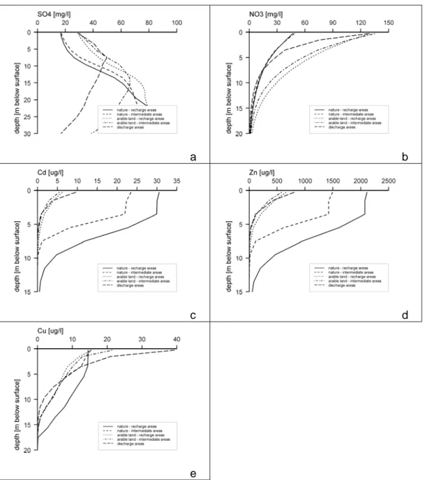
(7) 2.. Report with results of groundwater flow and reactive transport modelling in Dutch part of the Meuse basin (TNO/UU). A. Visser1, R. Heerdink2, H.P. Broers2 & B. van der Grift2 1 Department of Physical Geography, Utrecht University 2 TNO - Environment and Geosciences TNO - Environment and Geosciences Princetonlaan 6 / P.O. Box 80015 3508 TA Utrecht, The Netherlands Tel: +31 30 2564750 Fax: +31 30 2564755. h.broers@tno.nl 2.1. Introduction. Trends in groundwater quality are determined by 1) trends in concentrations in recharging groundwater, 2) travel time of contaminant transport by groundwater flow, and 3) interactions with the subsurface. A three-dimensional reactive transport model is used for the trend detection and extrapolation of groundwater and surface water quality in the Dutch part of the Meuse basin within the scope of the TREND 2 workpackage. The three factors determining groundwater quality are combined in the three-dimensional reactive transport model. The three-dimensional reactive transport model we used is the Integrated Transport Model, developed by TNO and KIWA. It combines a stationary groundwater flow model (MODFLOW) with a three-dimensional multi-species transport model (MT3DMS). The model covers a rectangular area of 34.5 km (East-West) by 24 km (North-South) south of the city of Eindhoven (Figure 2.1a). The model area was classified into 5 classes according to land use and hydrology to calculate the initial chemical composition of groundwater (Figure 2.1b).. a. b. Figure 2.1: Spatial extent of the three-dimensional reactive transport model (a) and the 5 land use and hydrology classes (b).. 2.2. Results. Modeled concentration-depth profiles Depth profiles of modeled concentrations of sulfate, nitrate, cadmium, zinc and copper, for each of the 5 land use/hydrology classes, illustrate the effect of the three factors controlling the concentrations of contaminants in groundwater (Figure 2.2). Differences between the profiles are caused by differences in input between land use classes (agriculture or nature), 7.

(8) differences in travel times (recharge, intermediate or discharge) or by differences in chemical interactions between the pollutants and the subsurface.. a. b. c. d. e Figuur 2.2: Modeled concentration-depth profiles of sulfate (a), nitrate (b), cadmium (c), zinc (d) and copper (e) in the 5 land use/hydrology classes.. For the concepts used in analyzing concentration-depth profiles, the reader is referred to deliverable T2.3. In general, groundwater age increases with depth, which determines the concentration-depth profile with young water at shallow depth and older water at larger depth. Sulfate was transported conservatively by groundwater flow and differences between the five sulfate concentration profiles (Figure 2.2a) are the result of different concentrations in recharging groundwater and differences in groundwater flow velocity. Before the 1980s, sulfate input was primarily caused by atmospheric deposition, which was higher on natural land. As a result, sulfate concentrations below a depth of 15 meter were higher under natural land than under agricultural land. Since the 1980s sulfate enters the groundwater system largely through manure on agricultural land and, as a result, concentrations in agricultural areas are higher than in natural areas above 15 meter below the surface.. 8.

(9) Without nitrate reduction, the nitrate profiles (Figure 2.2b) would resemble the profiles of sulfate, which has a similar input history. However, nitrate is reduced in the saturated zone by a reaction with pyrite in the subsurface. Differences between nitrate profiles of each class were only the result of differences in input and travel time, because we assumed a homogeneous reactivity of the subsurface. Little nitrate enters the system in natural areas, but high concentrations were modeled beneath agricultural land. In recharge areas groundwater flow is faster than in intermediate areas and nitrate reached deeper parts of the aquifer slightly quicker. In discharge areas, high concentrations at the surface are reduced by mixing with old water with no nitrate at greater depths. Concentration-depth profiles of heavy metals (Figure 2.2c, d and e) showed different patterns as a result of sorption to soil particles, such as clay and organic matter. Agricultural soils are richer in organic matter to which heavy metals sorb and as a result the heavy metals are retained in the topsoil in these areas. Natural soils generally have lower organic matter contents and lower pH values and heavy metals are more mobile and reach deeper parts of the aquifer. Copper (Figure 2.2e) is strongly adsorbed to soil particles in dry soils and only when high groundwater levels occur, as in discharge areas, copper is released under anoxic condictions to the upper groundwater in large amounts.. Tongelreep. Strabeekse-Aa Run. BeekloopKeersop Dommel. Kleine-Aa. Figuur 2.3: Catchments in the model area.. 9.

(10) Modeled breakthrough curves in streams Retardation of heavy metals also affects breakthrough curves in streams. To illustrate this effect we modeled the breakthrough of a block front of diffuse pollution of a conservative substance (Figure 2.4a) in the Run catchment (Figure 2.3) and compared it to the breakthrough curve of zinc, which is adsorbed and retarded (Figure 2.4b). The block front of pollution started in 1950 and stopped in 1970. The concentration of the conservative substance quickly increases, and decreases after input is stopped. The concentration of zinc slowly increases, but concentrations in the stream keep rising and remain high as a result of the retarded release of accumulated zinc in the subsoil. This difference is essential to predict the effect of regulatory measures to reduce pollution loading.. a b Figure 2.4: Model predicted breakthrough of a 20 year conservative block front of Cinput = 1000 mg/l in the Run catchment (left) and retarded breakthrough of zinc (right) for the period 1950-2050.. Effects of regulatory measures Because manure today is the most important contributor to diffuse pollution from agriculature, one would expect that stopping the use of manure would dramatically improve the quality of groundwater and surface water. We tested the effect of a zero emissions scenario (no use of manure) by modeling the concentrations of pollutants in surface water under such a regime. We found that only for conservative pollutants (such as SO4) the surface water quality improves within a short time frame (Figure 2.5a). If the pollutant is degraded (such as denitrification of nitrate) this effect is enhanced. (Figure 2.5b) However, for pollutants which have accumulated in the subsurface (such as Cd, Zn and Cu), stopping the input at the surface has very little to no effect in the next 50 years on the discharge of these pollutants into surface water by groundwater (Figure 2.5c,d and e).. 10.

(11) a. b. c. d. e Figure 2.5: Groundwater contribution to surface water for sulfate (a), nitrate (b), cadmium (c), zinc (d) and copper (e) between 1950 and 2050 in the Run catchment as a result of no changes in future land use (black) and a zero-emissions of manure after 2005 scenario (blue).. 2.4. Conclusions. Three-dimensional reactive transport modeling is useful to determine the current state of the groundwater system, as well as to predict the reaction of the groundwater system to regulatory measures aimed at improving groundwater quality. Modeled concentration-depth profiles show the amount and location of the pollutants in the groundwater body and are consistent with measured profiles. (See also T2.3 for measured profiles and T2.6 for the comparison between measured and modeled profiles) Breakthrough curves of pollutants in surface water show that despite drastic regulatory measures (completely abandoning manure practices), the delivery of heavy metals by groundwater to the surface water will continue to increase for the next 40 years as a result of the leaching of the accumulated stock of heavy metals in the soil.. 11.

(12) 3.. Report with results of groundwater flow and reactive transport modelling in the Geer catchment (ULg). Ph. Orban1, S. Brouyère1, 2 1 Group of Hydrogeology and Environmental Geology 2 Aquapôle Ulg University of Liège, Building B52/3, 4000 Sart Tilman, Belgium Tel: +32.43.662377 Fax: +32.43.669520 Serge.Brouyere@ulg.ac.be. 3.1. Introduction. In the framework of the AquaTerra project, HG-ULg has developed a methodology using statistical approaches to infer trends in nitrate groundwater quality for different sub-basins of the Meuse River. Following the development of this methodology, HG-ULg is developing a groundwater flow and solute transport model as a prediction tool for trend analysis in one of these sub-basins, the Geer Basin. New concepts for large-scale transport modelling, more particularly a modelling approach, the Hybrid Finite Element Mixing Cell (HFEMC) developed by HGULg and implemented in the 3D simulator SUFT3D (Deliverable R3.18) are used to develop this model. During the last months of the project, HG-ULg activities were:  interpreting the results of a tritium survey realised in the Geer basin  improving the conceptual model and updating the 3D finite element mesh for a better representation of the delay in infiltration of water and nitrate across the thick unsaturated zone of the Geer basin;  performing validation tests of the distributed mixing cell approach planned for the nitrate transport simulations;  performing various runs with the model.. 3.2. Interpretation of the tritium survey. Different authors (Broers, 2004; Koh et al. 2006) have highlighted the importance of water age for the understanding of diffuse pollution. The spatial distribution of groundwater age is a key factor determining the distribution of solute in groundwater. In parallel of the study of the nitrate pollution in the Geer basin, HGULg has taken samples for tritium analysis. Tritium concentrations measured in groundwater samples range from the detection limit to 14.7 TU (Figure 3.1). Roughly, three zones can be distinguished from the tritium concentrations:  A zone in the North of the Basin (confined part of the Hesbaye aquifer) where tritium concentrations are very low, close to 1. Such concentrations are characteristic of water infiltrated before the 1960.  A zone in the South-West of the basin where the tritium concentrations are high, ranging from 5 to 14 TU. Such concentrations are usually characteristic of water infiltrated after 1960.  A zone located in the East and North-East of the basin where tritium concentrations range from 2 to 6 TU-). These concentrations are probably characteristic of mixing between water infiltrated before and after the sixties. These three zones can also be distinguished in the spatial distribution of nitrate concentrations (Figure 3.2).. 12.

(13) Figure 3.1: Tritium units measured in the groundwater samples from the Geer basin. Figure 3.2: Nitrate units measured in the groundwater samples from the Geer basin. The relatively coherent correspondence between tritium and nitrate “spatial trends” in the basin allows one to propose the following interpretation:  The South-West of the Geer basin mostly correspond to the recharge zone of the aquifer, with younger more contaminated water.  The North-East of the Geer basin corresponds to the discharge zone of the aquifer (in particular in the Geer River), with a mixture of old water that have traveled all across the aquifer and recent water directly recharged in the area.. 13.

(14) . In the confined part of the aquifer (North of the Geer basin), groundwater is still uncontaminated because it has not been reached yet by the nitrate contamination front.. In terms of modelling, a first interpretation was performed using black box models by the Laboratory of Environmental Isotopy (Prof. P. Maloszewski, Dr W. Stichler), GSF-Institute of Groundwater Ecology in Munich (Germany). Collected isotopic data were modeled by GSF using the FLOWPC code developed by Maloszweski and published by IAEA (IAEA, 2002) for the interpretation of environmental tracer data. This code includes different analytical solutions such as the piston flow model, the dispersion model… On the basis of the tracer concentration in the infiltration and the observed concentrations at the different sampling points and for a chosen model, it is possible to compute, by an inverse procedure, the parameters defining the model. For example, using the dispersion model, GSF has computed apparent transit time ranging from 80 years to more than 200 years. However, these results have to be put into perspective and taken with great caution. Indeed, whatever the selected modelling approach, it is a very rough representation of the hydrogeological conditions prevailing in the Geer basin. In particular, many authors (e.g. Zoellmann et al. 2001; Koh et al. 2006) highlighted the difficulty in interpreting isotopic data in complex media (unsaturated zone with variable thickness, double porosity media…) with simplified analytical solutions. An alternative will be to use numerical distributed groundwater flow and solute transport models such as the SUFT3D model developed for the Geer basin in the framework of the AquaTerra project.. 3.3. Improvement in the conceptual model developed for the Geer basin. In the previous conceptual model developed for the Geer basin (Deliverable R3.18) the loess layer surmounting the chalky aquifer was not represented in the model. The water and nitrate fluxes leaching through the loess were computed by the EPIC-Grid soil model (UHAGx team). As explained in the previous deliverables this loess layer plays a key role in the transmission of nitrate from the surface to the aquifer. The improved conceptual model includes this loess layer explicitly in the model for two reasons:  After the review of the water and nitrate fluxes computed by the EPIC-Grid soil model, it appears that the nitrate concentrations computed by the code at the top of the model are too low (Figure 3.3) to explain the nitrate concentration measured in the groundwater. This is probably inherent in the fact that the EPIC-Grid code is mainly a soil model, poorly adapted to the computation of nitrate fluxes to the depth. It is thus better to use values of nitrate fluxes computed at the bottom of the root zone or to use estimated values while waiting for more accurate data.  HG-ULg has performed a tritium survey in the Geer Basin. The tritium concentration in the recharge can be easily estimated and is considered to be constant for the whole basin. The results of these surveys could be used in the regional calibration of the transport model provided that this model integrates the whole unsaturated zone.. 14.

(15) Figure 3.3: Nitrate concentration computed by the EPIC-Grid soil model in function of depth (from PIRENE, 2004, UHAGx). The updated model has been divided into five layers of finite elements (instead of three in the previous version): one layer for the bottom chalk aquifer, two for the upper chalk aquifer and two for the loess layer. The upper chalk and the loess layers are modelled using two layers of finite elements to better represent the variations of groundwater levels in the unsaturated zone (Figure 3.4). The new model is made of 12690 nodes and 19960 triangular elements with a mean side of 500 meters. All the other conceptual choices are similar to those presented in the Deliverable R3.18.. 15.

(16) Figure 3.4: 3D-Mesh, the different colours correspond to the materials (vertical scale multiplied by100). 3.4. Validation tests of the distributed mixing model implemented in the SUFT3D code. Different tests have been performed to verify that the distributed mixing cell approach (Campana et al., 1984; Harrington et al., 1999) is correctly implemented in the SUFT3D code. Under few simplifying assumptions, the equation describing the distributed mixing model (Equation 9 in Deliverable R3.18) can be solved semi-analytically. To validate the implementation of this model in the SUFT3D code, a one-dimensional solution has been evaluated. A solute is supposed to be injected with a unitary concentration in a column divided in mixing cells connected in series. The flow is steady state and a constant recharge of 110-6 is prescribed at the top of the column. The solute is injected in the fluid entering the column. The section perpendicular to the flow is unitary; the height of each cell is 0.1 m. The effective volume of water in each cell is equal to 10% of the total volume of the cells. The spatial and temporal evolution of the concentration in a column of 100 mixing cells is then computed with the SUFT3D code under the same assumptions. The mass balance equation as applied to a mixing cell i (Figure 3.5) can be written:. Vi. d Ci  Qii1C i 1  Qii 1C i dt. where Vi (L³) is the mixing volume associated to the mixing cell i, the terms Qii1 (L³T-1) is the flow rate between the cell i and the upstream cell i-1, Qii 1 (L³T-1) is the flow rate between the cell i and the downstream cell i+1, C i (ML-3) is the concentration in the mixing cell i, Ci 1 (ML3 ) is the concentration in the upstream cell i-1.. 16.

(17) Qii1. Qii. Ci. Ci 1. Ci1. Vi Figure 3.5: Scheme of the mixing cells used for the validation test. As the flow is steady state, Qii1  Qii 1  Qin and the mixing equation becomes:. Vi. d Ci  Qin C i 1  C i  dt. An approximate solution can be easily derived, expressing the evolution of the concentration in the mixing cell i. The temporal derivative is approximated by a finite difference scheme; the other terms of the equation being estimated explicitly. The discrete form of the equation is:. Vi. C i (t  t )  C i (t )  Qin C i 1 (t )  C i (t )  t. The evolution of the concentration in the cell i can be computed as follow:. C i (t  t ) . Qin t Ci 1 (t )  Ci (t )   Ci (t ) Vi. In Figure 3.6 and 3.7, the concentrations computed with the semi-analytical solution (continuous line) and the SUFT3D (symbols) are compared. The concordance is perfect, confirming the precision of the approach implemented in the code.. 17.

(18) Figure 3.6: Spatial comparison between the results of the mixing cell model implemented in the SUFT3D code and the one-dimensional semi-analytical solution.. Figure 3.7: Temporal comparison between the results of the mixing cell model implemented in the SUFT3D code and the one-dimensional semi-analytical solution.. 3.5. Latest development of the groundwater flow model. During the last months, the groundwater flow model has been run under different scenarios. The introduction of very thin elements (representing the loess) has led to non-convergence problems with the flow simulations. It has turned out that the problem was related to the occurrence of negative transmissibility values related to the flatness of the finite elements. To fix this problem, the code has been modified to calculate elemental integrations on tetrahedral sub-elements following the recommendations of Letniowski et al., 1991. Debugging operations have been completed recently and first simulations of the Geer groundwater model indicate a major improvement in the convergence of computations.. 3.6. Next steps. The model still has to be calibrated in transient conditions. However, it can already be used for running first nitrate transport scenarios in the framework of the TREND T2 sub-project. For example, it could be an interesting exercise to model transient nitrate fluxes recharge under mean steady state groundwater flow conditions. Trend analysis results presented in deliverable T2.4 and the results of the two tritium surveys will be used as calibration and validation datasets for the groundwater flow and transport model. Then the model will be used to perform trend forecasting. Results of this work will be submitted within deliverable T2.10. The model could be used to simulate the fate of other contaminant (for example PAH) as far as the appropriate data (deposition and rate of infiltration, sorption data) could be provided and be representative for the whole Geer Basin. Collaborations within Aquaterra between COMPUTE research groups (in particular the University of Tübingen) and HGULg consist in testing the various tools proposed by the 18.

(19) COMPUTE partners by developing common applications on the Geer basin. Different data have already been exchanged. In a near future, the different teams would like to compare the different modelling approach developed on the Geer Basin case study. In the future it is also expected to use the calibrated groundwater model for a collaboration with INTEGRATOR on the socio-economical analysis of the nitrate problem in the Geer basin.. 19.

(20) 4.. Report with results of groundwater flow and reactive transport modelling at selected test locations in the Brévilles' catchment (BRGM). Surdyk N., Dubus I.G. & Gutierrez A. BRGM Avenue C. Guillemin BP 6009 45060 Orléans Cedex 2 France T: +33 (0)2 38 64 47 50 F: +33 (0)2 38 64 34 46 i.dubus@brgm.fr. 4.1. Introduction. The modelling of pesticide concentrations at the Brévilles spring is considered to be a complex undertaking as patterns of pesticide concentrations in water are the results of an integration of transfers through a range of environmental compartments. We adopted an approach where results from an appropriate 1D soil leaching model (MACRO) are fed into a 2D saturated zone model (MARTHE) (Figure 4.1). The MACRO running and the extraction of relevant data to be used as inputs in MARTHE have been fully automated. Field 1 agronomical data MACRO 1D Simulations. GIS integration. Field 2 agronomical data. Field 1 agronomical data. Soil 2 data. Soil 1 data. Field 1 × Soil 1 lt. Field 2 agronomical data. Field 2 × Soil 1 lt. MARTHE simulations. Field 2 × Soil 2 lt. Field 1 × Soil 2 lt. Concentration and flux at the spring 2D simulation. Figure 4.1: Modelling methodology. The field leaching model requires agronomic and crop protection data on a field-by-field basis over a significant number of years, as well as soil data at such a spatial resolution. The scale of running for MACRO is therefore the field x soil scale over the 330 ha Brévilles catchment (Figure 4.2). MACRO results for one particular field x soil combination are assumed to be homogeneous within the zone, i.e. the spatial variability within each zone is neglected. Outputs of interest from the leaching model include i) predictions for percolation at the bottom of the leaching column and ii) concentrations of pesticides in leachate.. 20.

(21) 4.2. First results. First simulations display differences in cumulated volumes of percolated water simulated by MACRO between 1988 and 2004. 4581 mm of cumulated percolated water have been simulated for the driest combination (soil  field) while 5726 mm of cumulated percolated water were predicted for the wettest combination. Predictions of cumulated percolated water were found to be impacted by soil types and fields (Figure 4.2) a. Cumulated water (mm) 4581. 4600-4800 4800-5000 5000-5200 5200-5400 5400-5695. b. c 5726. Figure 4.2: Maps of fields (a), soils (b) and predicted recharge (c) at Brévilles between 1988 and 2004.. More cumulated percolated water is simulated in soil 4 and less in soil 2 at a depth of 50 cm. At a depth of 20 m, the predicted volumes are more important for soil 3 and still the lowest for the soil 2. Percolation was found to be fast under the forest cover (field 33) in the first 50 cm and almost the slowest after 20 m (Figure 4.3). 6500 5726. 5800 5600 5400 5200 5000 4800 4600 4581. 4400 4200 4000. 1 2 3 4 5 6 7 8 9 10 11 12 13 14 15 16 17 18 19 20 21 22 23 24 25 26 27 28 29 30 31 32 33. Soil2. Soil3. 6465. 6300 6100 5900 5700 5500 5300 5100 4900 4700. 4772. 4500 1 2 3 4 5 6 7 8 9 10 11 12 13 14 15 16 17 18 19 20 21 22 23 24 25 26 27 28 29 30 31 32 33. Field Soil1. Cumulated water leaching at 20 m (mm). Cumulated water leaching at 50 cm (mm). 6000. Field. Soil4. Soil1. Soil2. Soil3. Soil4. Figure 4.3: Cumulated water leaching simulated by MACRO at a 50 cm depth between 1988 and 2004. The chart show results obtained for each of the 33 individual fields for the 4 soils. The X numbers refer to the field label as presented on Figure 4.3a. Atrazine was applied in 10 fields, but the initial modeling predicted that the compound would reach 50 cm in detectable amount in 3 fields only. The initial parameterization also suggested that leaching at 6 m would only occur in one filed only (Figure 4.4).. 21.

(22) Average concentration of atrazine at 6 m (µg/l). Average concentration of atrazine at 50 cm (µg/l). 2.0E-01. 1.6E-01 1.4E-01 1.2E-01 1.0E-01 8.0E-02 6.0E-02 4.0E-02 2.0E-02. 1.8E-01 1.6E-01 1.4E-01 1.2E-01 1.0E-01 8.0E-02 6.0E-02 4.0E-02 2.0E-02 0.0E+00. 0.0E+00. 0 1 2 3 4 5 6 7 8 9 101112131415161718192021222324252627282930313233. 0 1 2 3 4 5 6 7 8 9 101112131415161718192021222324252627282930313233. Field. Field Soil 1. Soil 2. Soil 3. Soil 4. Soil 1. Soil 2. Soil 3. Soil 4. Figure 4.4: Average concentration of atrazine between 1988 and 2004 for each field and soil. The arrows indicate fields which received atrazine applications. The X numbers refer to the field label as presented on Figure 4.3a.. Figure 4.5 shows predicted atrazine daily concentration in leaching at a depth of 50 cm for field #13. This field is of particular interest because it contains the 4 soils and received 3 atrazine applications over the study period. Leaching profiles for the 4 soils were predicted to be significantly different (Figure 4.5). Also, losses were much more significant for the third application despite the application rate being only marginally larger. This highlights the importance of climate characteristics.. 160 140 120 100 80 19 apr 1994 1000 l/ha. 60. 16 mar 1996 1000 l/ha. 19 mar 1998 1250 l/ha. 40. 07/01. 01/01. 07/00. 01/00. 07/99. 01/99. 07/98. 01/98. 07/97. 01/97. 07/96. 01/96. 07/95. 01/95. 07/94. 01/94. 0. 07/93. 20 01/93. Average daily concentration of atrazine (µg/l). 180. date Soil 1. Soil 2. Soil 3. Soil 4. Figure 4.5: Atrazine concentrations predicted for field #13 between 1993 and 2001 for the 4 soils at a depth of 50 cm.. – Predicted concentrations of atrazine were smaller at a 6-m depth (Figure 4.6). The differences of predicted concentrations between soil 4 and the others were more important than at a depth of 50 cm. The differences between the soil 2 and the soil 3 were also more important. Six months were needed to reach a concentration close to 0 at 50 cm while more than 4 years were needed to reach the same concentration at 6 m.. 22.

(23) 0.3 0.25 0.2 0.15. 16 mar 1996 1000 l/ha. 19 apr 1994 1000 l/ha. 19 mar 1998 1250 l/ha. 0.1 0.05. 07/01. 01/01. 07/00. 01/00. 07/99. 01/99. 07/98. 01/98. 07/97. 01/97. 07/96. 01/96. 07/95. 01/95. 07/94. 01/94. 07/93. 0 01/93. Average daily concentration of atrazine (µg/l). 0.35. date Soil1. Soil 2. Soil 3. Soil 4. Figure 4.6: predicted atrazine concentrations for field #13 between 1993 and 2001 for the 4 soils at a depth of 6 m.. Predicted Atrazine concentrations are higher for the soil 4 because it is the sandiest and the shallowest soil.. 4.3. Conclusion. First results with regard to the predictions of the transfer of water and atrazine in the unsaturated zone at Brévilles were obtained. These results will be fed automatically into the 2D saturated zone model MARTHE and calibration activities will then be undertaken to try to match observed leaching data and associated concentrations at the Brévilles spring. First results for atrazine leaching are considered to be rather low and the parameterization of the MACRO model will be adjusted accordingly. The overall running period will be extended to encompass the transfer times from the soil surface to the saturated zone.. 23.

(24) 5.. Discussion. This report describes the results of the modeling effort in the Dommel (TNO/UU), Geer (ULg) and Brévilles (BRGM) catchments. The aim of the deterministic modeling effort is trend detection and extrapolation of concentrations of contaminants in the catchments under study. The results of the trend detection and extrapolation will be reported in the next Deliverable (T2.10). The results in this deliverable show that the deterministic models are capable of capturing the variation and dynamics of three-dimensional reactive transport of contaminants. Modeling results for potassium, nitrate, cadmium, zinc and atrazine illustrate the nonconservative behavior of these contaminants: retardation affects zinc transport, denitrification may affect nitrate transport in anoxic parts of the aquifer and retardation and decay affect atrazine transport. Also, the model results clearly show the effect of land use, soil type and hydrology on the transport of contaminants towards and in the groundwater system and back to surface water systems (Figure 2.2, 3.2 and 4.6). These results are promising for the next step of the AquaTerra TREND 2 reseach: detecting trends in groundwater quality by using reactive transport models. Also, these models have excellent capability of extrapolating these trends into the future, and assessing the effect of regulatory measures to reduce the contamination of the groundwater bodies. Results of this research will be reported in Deliverable T2.10. Finally, the different statistical methods of trend detection, as well as the different reactive transport models used for trend detection and extrapolation will be compared in terms of data-requirement, costs and accuracy, to be reported in Deliverable T2.11 and a joint scientific publication of all TREND 2 partners. These findings will be interesting for the FLUX work package, concerning the fluxes of pollutants from groundwater to surface water, as well as the INTERGRATOR and EUPOL work packages to analyze the socio-economical aspects of the nitrate problem in the Geer basin and the implementation of cost effective and accurate methods for trend detection and demonstration of trend reversal to be used by stakeholders to comply with the upcoming EU Groundwater Framework Directive.. 24.

(25) References Heerdink, R., Van der Grift, B., Broers, H.P., Marsman, A., Roelofsen, F., (2006. ) Aquaterra/Stromon Intermediate Report II: pilot model study in Southeast Brabant (in Dutch). TNO-report. Broers, H.P., A. Marsman, F.C. van Geer, B. van der Grift & A. Visser (2007) Improving the prediction of future groundwater quality by analyzing concentration-depth profiles. Proceedings paper submitted to Water Rock Interaction 2007. H.P. Broers, B. van der Grift, J. ,Griffioen, J. en Heerdink R. (2007) Modelling reactive transport of diffuse contaminants in groundwater: identifying the groundwater contribution to surface water quality. Chapter 10.2 in Groundwater Science & Policy, edited by Ph. Quevauviller. Published by Royal Society Chemistry. Pages 636-651. Floris Verhagen, Hans Peter Broers, Andries Krikken, Joachim Rozemeijer, Remco van Ek, Michelle van Vliet, Bas van der Grift, Ruth Heerdink, 2007. Groundwater - Surface Water Interaction: Regional differences in Noord Brabant (in Dutch). Report by TNO and Royal Haskoning (draft 3). Broers H.P, Visser A., Heerdink, R, Van der Grift, B., Surdyk N., Dubus I.G., Gutierrez A., Orban, Ph., Brouyere, S., 2007. TREND 2.7. Short report describing the progress of the groundwater flow and reactive transport modeling and elucidating interactions with COMPUTE and HYDRO and FLUX work packages Broers H.P, Visser A., Van der Grift, B, Dubus I.G., Gutierrez A., Mouvet C., Baran N., Orban, Ph., Batlle Aguilar J., Brouyere S., 2006. TREND 2.5: Input data sets and short report describing input data for groundwater and reactive transport modelling at test locations in Dutch part of the Meuse basin, the Brévilles' catchment and the Geer catchment. Broers, H.P. & A. Visser eds.(2005) Report on extrapolated time trends at test sites AQUATERRA report Deliverable T2.4, 81 p. Broers, H.P. & A. Visser eds.(2005) Report on concentration-depth, concentration-time and time-depth profiles in the Meuse basin and the Brévilles catchment AQUATERRA report Deliverable T2.3, 69 p. Broers, H.P. & A. Visser eds. (2005) Report with documentation of reconstructed land use around test sites AQUATERRA report Deliverable T2.2. 64 p Broers, H.P. & A. Visser eds.(2004) Documented spatial data set containing the subdivision of the basins into groundwater systems and subsystems, the selected locations per subsystem and a description of these sites, available data and projected additional measurements and equipment. AQUATERRA report Deliverable T2.1 Campana M.E., Simpson E.S. (1984), Groundwater residence times and discharge rates using discrete-state compartment model and 14C data, J. Hydrol., 72, 171-185. Harrington G.A., Walker G.R., Love A.J., Narayan K.A. (1999), A compartmental mixing-cell approach for the quantitative assessment of groundwater dynamics in the Otway Basin, South Australia, J. Hydrol., 214, 49-63. IAEA (2002). Use of isotopes for analyses of flow and transport dynamics in groundwater systems, IAEA-UIAGS.. 25.

(26) Koh, D.-C., L. N. Plummer, D. K. Solomon, E. Busenberg, Y.-J. Kim and H.-W. Chang (2006). "Application of environmental tracers to mixing, evolution, and nitrate contamination of ground water in Jeju Island, Korea." Journal of Hydrology 327: 258-275. Letniowski F.W., Forsyth P.A. (1991) A control volume finite element method for threedimensionnal NAPL groundwater contamination, Int. J. Num. Met. Fl., 13, 955-970. Zoellmann, K., W. Kinzelbach and C. Fulda (2001). "Environmental tracer transport (3H and SF6) in the saturated and unsaturated zones and its use in nitrate pollution management." Journal of Hydrology 240: 187-205.. 26.

(27)