Weakly Relational Numerical Abstract Domains
323
0
0
Texte intégral
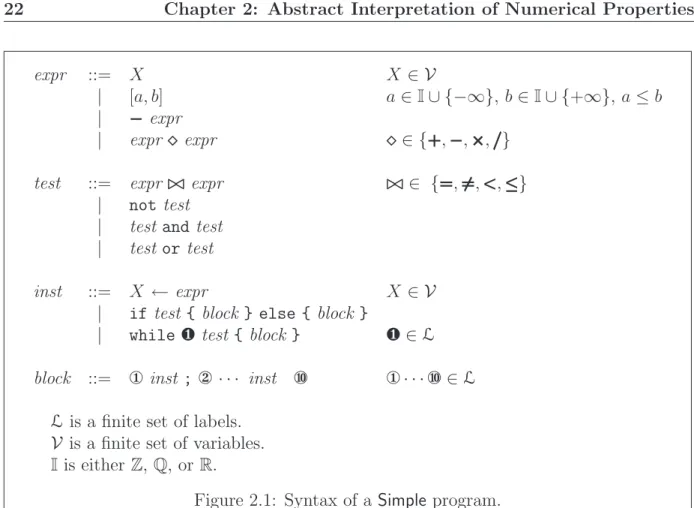
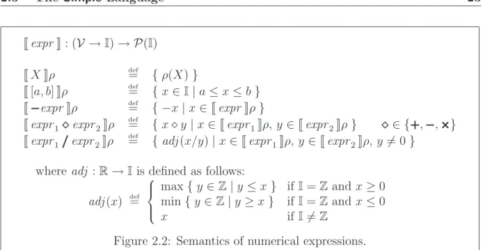
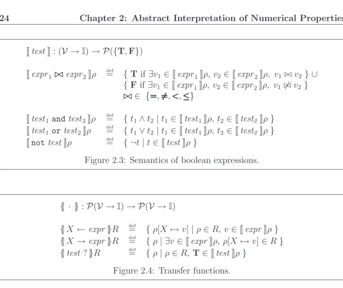
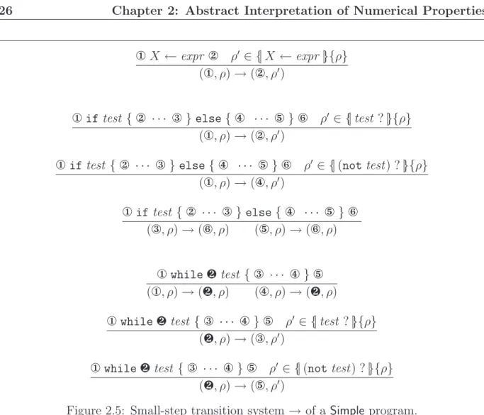
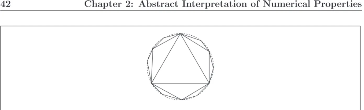
Figure
+7

Documents relatifs
