On some multi-phase problems in continuum mechanics

HAL Id: pastel-00923691

https://pastel.archives-ouvertes.fr/pastel-00923691

Submitted on 3 Jan 2014

HAL is a multi-disciplinary open access

archive for the deposit and dissemination of

sci-entific research documents, whether they are

pub-lished or not. The documents may come from

teaching and research institutions in France or

abroad, or from public or private research centers.

L’archive ouverte pluridisciplinaire HAL, est

destinée au dépôt et à la diffusion de documents

scientifiques de niveau recherche, publiés ou non,

émanant des établissements d’enseignement et de

recherche français ou étrangers, des laboratoires

publics ou privés.

On some multi-phase problems in continuum mechanics

Stefano Bosia

To cite this version:

Stefano Bosia. On some multi-phase problems in continuum mechanics. Mechanics of materials

[physics.class-ph]. Ecole Polytechnique X, 2013. English. �pastel-00923691�

Politecnico di Milano

Department of Mathematics

Doctoral Programme in

Mathematical Models and Methods in Engineering

École Polytechnique

LMS - Laboratoire de Mécanique des Solides

Granted by Università italo francese, Bando Vinci 2011

On some multi-phase problems

in continuum mechanics

Doctoral Dissertation of:

Stefano Bosia

Advisors:

Prof. Maurizio Grasselli

Prof. Andrei Constantinescu

Tutor:

Prof. Filippo Gazzola

Chair of the PhD Program:

Prof. Roberto Lucchetti

Committee:

Prof. Maurizio Grasselli

Prof. Andrei Constantinescu

Prof. Ferdinando Auricchio

Prof. Tomás Caraballo

Prof. Giuseppe Geymonat

Prof. Dietmar Hömberg

Referees:

Prof. Tomás Caraballo

Prof. Alexander Korsunsky

Synopsis

In this thesis we study some problems arising within the context of continuum mechanics in the description of multi-phase physical situations. This analysis is carried out by means of tools from the theory of dynamical systems More precisely, we consider the following three problems: (I) the flow of binary mixtures, (II) p-n junctions in semiconductors under strain and (III) fatigue in polycrystalline metals.

On the flow of binary mixtures. The flow of binary mixtures can be described by two variables: the velocity of the medium u and an order parameter ψ. This last represents the difference in the relative concentrations of the two constituents of the mixture. The basic model we consider is the well known model H

$ ’ ’ ’ ’ ’ ’ ’ ’ & ’ ’ ’ ’ ’ ’ ’ ’ % Btu` pu · ∇qu “ ´∇π ` ∇ · pτ pDu, ψqq ´ ε∇ · p∇ψ b ∇ψq ` gptq ∇· u“ 0 Btψ` pu · ∇qψ “ ∇ · pM∇µq µ“ ε´1_f1_{pψq ´ ε∆ψ.}

Here fpψq is a double-well potential describing the natural separation tendency of the two com-ponents of the fluid. This system is an example of a diffuse interface model for binary flows, a class of models, which has been proven to be effective for numerical simulations and applica-tions. In Chapter 1, we account for the models considered and we briefly review the theory of infinite-dimensional dynamical systems used in the rest of the first part. In particular, we prove the following

• For non-newtonian fluids (shear-thickening fluids of Ladyzhenskaya type) on a bounded

Synopsis-2

main of R3_{and for a singular (i.e. logarithmic) double-well potential, we prove the existence}

of solutions and the existence of a trajectory attractor (Chapter2).

• For the original model H on a bounded domain of R2_{with a polynomial potential, we show}

the existence of a pullback exponential attractor. In particular, we explicitly account for arbitrarily fast growth of the potential at infinity. Although we are able to deduce results on the asymptotic behaviour of the system without limitations on the growth of the potential, the estimates we deduce are not strong enough to pass to the limit for regular potentials converging towards singular ones (Chapter3).

• We then enquiry the effects of a reaction term on the behaviour of the binary fluid. This can be seen as a model describing chemically reacting fluids, whose average composition might vary over time. In particular, we prove the existence and the uniqueness of solutions on bounded domains of R2_{for polynomial potentials. Moreover, we deduce the existence of}

a robust (with respect to the rate of the chemical reaction) family of exponential attractors (Chapter4).

• Finally we consider a non-local version of the Cahn-Hilliard equation with a singular inter-action kernel. This is a preliminary step in the study of a non-local model H with singular kernels. In the case of bounded domains in R3 _{with a singular potential, we prove the}

existence of variational solutions satisfying natural boundary conditions and study their regularity. Although the natural boundary conditions for the phase variable seems difficult to characterise in this setting, we are able to show that for regular solutions they reduce to the usual homogeneous Neumann (no flux) boundary conditions (Chapter 5).

Several interesting but challenging issues remain open, for instance:

• the study of the regularity properties and in particular the regularity up to the boundary for the non-local Cahn-Hilliard equation considered in Chapter5;

• the investigation of the well-posedness properties and the asymptotic behaviour of the non-local model-H with singular kernel;

• a further study of the long-term properties of the Navier-Stokes-Cahn-Hilliard-Oono sys-tem already treated in Chapter 4. In particular, the problem of the convergence towards stationary states for this system seems particularly worth investigation.

On the effects of strain on semiconductor-based p-n junctions. Semiconductor devices essentially operate using the differences in the physical properties of two sharply separated regions,

Synopsis-3

one rich in electrons and one rich in holes (or, equivalently, lacking of electrons), which can ideally be considered as two phases of a continuum. However, with respect to the previous part, in this case the position of the interfaces is in general a priori given by the knowledge of the doping profile of the semiconductor.

Here we are interested in studying how deformations affect the properties of semiconductors. Our line of reasoning is based on the following approach:

• we start by reviewing fundamental semiconductor physics both for intrinsic and for doped silicon (Chapter6).

• we then derive the drift-diffusion model and investigate which of its parameters depend on strain. Moreover, we give explicit models for the effects of strain on the band-gap width, on the mobilities and on the concentration of minority carriers in doped semiconductors (Chapter7).

• we derive the Shockley relation in dependence of strain. In particular, we discuss the relevance of the reverse coupling of electronic properties on mechanical deformations through Maxwell stresses and conclude that it can be neglected at first approximation (Chapter 8).

The analysis has shown that several questions have still to be answered as, for example:

• the construction of a complete thermodynamically consistent continuum model for the cou-pled electro-mechanical effects in semiconductors;

• a rigourous treatment through perturbation analysis of the strain at the p-n junction;

• applications to other device architectures such as transistors and sensors.

On the lifetime estimate in high cycle fatigue regime for alloys. In the last part, we apply the theory of finite-dimensional dynamical systems to the field of lifetime predictions of polycrystalline metals in the high cycle fatigue regime. The model we consider is based on a homogenisation procedure which will relate local strains and stresses in the elastic and plastified grains at the microscopic level with the global strain and stress at the scale of the structure. The fatigue predictions are carried out using techniques from dynamical systems to track the progress of the accumulated plastic deformation in the grains. The proposed model for fatigue lifetime predictions offers greater flexibility in accommodating experimental data than those al-ready presented in the literature. At the same time, it remains amenable to explicit analytical treatment.

Synopsis-4

• the investigation of the effects of stochastic terms and, in particular, the treatment of the resulting models within the framework of stochastic dynamical systems;

• the study of other loading regimes, such as quasiperiodic loadings or nondeterministic load-ings;

• the extension to shape memory alloys accounting for the phase change occurring in these materials.

Publications

Most of the results of this thesis are contained int he following research articles:

• S. Bosia, Analysis of a Cahn-Hilliard-Ladyzhenskaya system with singular potential, J. Math. Anal. Appl. 397 (2013) 307–321, Chapter2;

• S. Bosia, M. Grasselli, A. Miranville,On the longtime behavior of a 2D hydrodynamic model for chemically reacting binary fluid mixtures, Math. Methods Appl. Sci. (2013), Chapter4;

• S. Bosia, A. Constantinescu, Fast time-scale average for a mesoscopic high cycle fatigue criterion, Int. J. Fatigue 45 (2012), 39–47, Chapter9;

• S. Bosia, S. Gatti,Pullback exponential attractors for a Cahn-Hilliard-Navier-Stokes system in 2D, arXiv:1304.0933 (2013), submitted, Chapter3

• H. Abels, S. Bosia, M. Grasselli,Cahn-Hilliard Equation with Nonlocal Singular Free Ener-gies, arXiv:1311.3642 (2013), Chapter5.

• S. Bosia, A. Constantinescu, M. Jabbour, N. Triantafyllidis, On the modelling of strained semiconductors, in preparation, Chapters7–8.

Sinthèse

Cette thèse est dédiée à l’étude de certains problèmes de la mécanique des milieux continu qui apparaissent lors de la modélisation de systèmes multi-phase. Cette analyse est conduite grâce aux instruments de la théorie des systèmes dynamiques. Plus précisément, les trois problèmes suivant sont considérés : (I) l’écoulement de fluides binaires (II) les jonctions p-n à semi-conducteur soumises à déformations et (III) la fatigue dans les métaux polycristallins.

Sur l’écoulement de fluides binaires. L’écoulement d’un fluide binaire peut être décrit par deux variables : la vitesse du milieux u et un paramètre d’ordre ψ. Ce dernier représente la différence entre les concentrations relatives des deux composants du mélange. Le système fondamental que nous considérons est connu sous le nom de modèle H et peut être ecrit comme il suit : $ ’ ’ ’ ’ ’ ’ ’ ’ & ’ ’ ’ ’ ’ ’ ’ ’ % Btu` pu · ∇qu “ ´∇π ` ∇ · pτ pDu, ψqq ´ ε∇ · p∇ψ b ∇ψq ` gptq ∇· u“ 0 Btψ` pu · ∇qψ “ ∇ · pM∇µq µ“ ε´1_f1_{pψq ´ ε∆ψ.}

Ici fpψq est un potentiel à double puits qui décrit la tendance naturelle à la séparation des deux composants du fluide. Ce système est un exemple d’un modèle à interface diffuse pour fluides binaires, une famille de modèles qui s’est démontrée efficace pour les simulations numériques et pour les applications. Le premier chapitre de cette thèse présente les modèles considérés tout en fournissant une vue générale sur la théorie des systèmes dynamiques infini-dimensionnels utilisée au cours du reste de la première partie. Plus précisément, on prouve les résultats suivants :

Sinthèse-2

• pour des fluides non-newtoniens (fluides rhéoépaississant du type de Ladyzhenskaya) dans un domaine borné de R3 _{et dans le cas d’un potentiel singulier (c’est-à-dire logarithmique),}

on prouve l’existence de solutions et l’existence d’un attracteur de trajectoires (Chapitre2) ;

• dans le cas du modèle H originaire donné sur un domaine borné de R2 _{avec un potentiel}

polynomial, on prouve l’existence d’un attracteur pullback exponentiel. Plus précisément, on tien compte d’une croissance arbitrairement rapide du potentiel à l’infini. Tout en pou-vant déduire ces résultats de dynamique asymptotique sans limitations sur la croissance du potentiel, les estimations que nous dérivons ne sont pas suffisamment fortes pour passer à la limite pour suites de potentiels singuliers convergents à un potentiel singulier (Chapitre3) ;

• successivement, on étudie les effets d’un terme de réaction sur le comportement du fluide binaire. Ceci représente un modèle qui décrit des fluides réagissant chimiquement, dont la composition moyenne peut changer dans le temps. Plus précisément, en des domaines bornés de R2 _{et pour des potentiels polynomiaux, on prouve l’existence et l’unicité de solutions.}

On déduit aussi l’existence d’une famille robuste (par rapport à la vitesse de la réaction chimique) de attracteurs exponentiels (Chapitre 4) ;

• enfin, on considère une version non-locale de l’équation de Cahn-Hilliard qui présente un noyau d’interaction singulier. Ces résultats représentent un passage préalable pour l’étude d’un model H non-local avec noyaux singuliers. Dans le cas d’un domaine borné en R3

avec un potentiel singulier, on prouve l’existence de solutions variationelles satisfaisant les conditions aux limites naturelles et on étudie leurs régularité. Même si ces conditions aux limites naturelles pour le paramètre d’ordre semblent difficiles à caractériser, on démontre que, pour des solutions régulières, elles se réduisent aux usuelles conditions de Neumann homogènes (Chapitre 5).

Plusieurs problèmes intéressants et difficiles restent sans solution. Parmi ceci on rappelle :

• l’étude des propriétés de régularité et en particulier la régularité jusqu’au bord pour l’équa-tion de Cahn-Hilliard non-locale considérée au Chapitre 5;

• la réponse à la question si le modèle H non-locale est bien posé ou pas et l’examen de son comportement asymptotique ;

• une investigation ultérieure des propriétés asymptotiques du système de Navier-StokesCahn-Hilliard-Oono déjà étudié aux Chapitre 4. Plus précisément, le problème de la convergence des solutions aux états stationnaires parait particulièrement intéressant.

Sinthèse-3

Sur les effets des déformations sur les jonctions p-n à semi-conducteur. Les dispositifs électroniques travaillent on exploitant les différences entre les propriétés physiques de deux régions nettement séparées, l’une riche en électrons et l’autre riche en trous (ou bien, pauvre en électrons), qui idéalement peuvent être considérées comme deux phase d’un même milieu continu Tout-de-même, par rapport à la partie précédente de cette thèse, dans ce cas la position des interfaces est généralement donnée grâce à la connaissance du profil de dopage du semi-conducteur.

L’objet principal de notre étude est la compréhension de comment les déformations affectent les propriétés des semi-conducteurs. Notre approche se base sur les phases qui suivent :

• on commence par présenter les éléments de physique des semi-conducteurs soit pour le silicium intrinsèque, soit dopé (Chapitre6) ;

• par la suite, on dérive le modèle de diffusion-dérive et on étudie quels de ses paramètres dé-pendent des déformations. On donne aussi des lois explicites pour les effets des déformations sur l’intervalle de bande, sur les mobilités des porteurs de charge et sur les concentrations des porteurs de minorité dans les semi-conducteurs dopés (Chapitre7) ;

• on obtient la loi de Shockley en dépendance des déformations. En particulier, on discute l’importance des effets du couplage inverse entre les propriétés électroniques et les déforma-tions mécaniques (contraintes de Maxwell) et on déduit que ceux-ci peuvent être négligés en première approximation (Chapitre8).

Nos analyses laissent ouverte des nombreuses questions comme, par exemple :

• la construction d’un modèle continu complet, thermodynamiquement consistent pour les effets électromécaniques couplés dans les semi-conducteurs ;

• un traitement rigoureux des déformations à la jonction p-n par la théorie des perturbations ;

• les applications à autres dispositifs comme transistors et senseurs.

Sur l’estimation de la durée de vie des alliages en fatigue à grand nombre de cycles. Dans la dernière partie, on utilise la théorie des systèmes dynamiques fini-dimensionnels dans le contexte des prédictions de la durée de vie des métaux polycristallins suomis à un grand nombre de cycles de chargement. Le model que l’on considère se base sur une procédure de homogénéisation qui lie les contraintes et les déformations locales dans les grains élastiques et plastiques au niveau microscopique avec les déformations et les contraintes à l’échelle de la structure. Les prédictions de fatigue sont menées en utilisant des techniques de la théorie des systèmes dynamique qui permettent de tracer l’évolution des déformations plastiques cumulées dans les grains. Le modèle

Sinthèse-4

de fatigue proposé offre, en comparaison avec les résultats déjà connus, une plus grande flexibilité pour accommoder les données expérimentales. Au même temps, il reste accessible à une analyse explicite.

Des possibles développements de ces résultats sont :

• l’étude des effets de termes stochastiques et, en particulier, le traitement des modèles résul-tant dans le contexte de la théorie des systèmes dynamiques stochastiques ;

• l’examen d’autre genre d’histoires chargement, comme les chargements quasipériodiques ou les chargements non-déterministe ;

• l’extension de ces techniques aux alliages à mémoire de forme tenant compte des transition de phase qui se vérifient dans ces matériaux.

Publications

La plus grande partie des résultats de cette thèse sont contenus dans les articles suivants :

• S. Bosia, Analysis of a Cahn-Hilliard-Ladyzhenskaya system with singular potential, J. Math. Anal. Appl. 397 (2013) 307–321, Chapitre2;

• S. Bosia, M. Grasselli, A. Miranville,On the longtime behavior of a 2D hydrodynamic model for chemically reacting binary fluid mixtures, Math. Methods Appl. Sci. (2013), Chapitre4;

• S. Bosia, A. Constantinescu, Fast time-scale average for a mesoscopic high cycle fatigue criterion, Int. J. Fatigue 45 (2012), 39–47, Chapitre9;

• S. Bosia, S. Gatti,Pullback exponential attractors for a Cahn-Hilliard-Navier-Stokes system in 2D, arXiv :1304.0933 (2013), soumis à comité de lecture, Chapitre3

• H. Abels, S. Bosia, M. Grasselli,Cahn-Hilliard Equation with Nonlocal Singular Free Ener-gies, arXiv :1311.3642 (2013), soumis à comité de lecture, Chapitre5.

• S. Bosia, A. Constantinescu, M. Jabbour, N. Triantafyllidis, On the modelling of strained semiconductors, en préparation, Chapitres 7–8.

Sintesi

Lo scopo di questa tesi è lo studio di alcuni problemi che traggono origine dalla descrizione di processi fisici multifase nel contesto della dinamica dei continui e che possono essere affrontati con strumenti della teoria dei sistemi dinamici. In particolare verranno considerate le seguenti tre situazioni: (i) la dinamica di fluidi binari (ii) le proprietà dei semiconduttori inorganici sottoposti a deformazioni e (iii) la fatica in metalli policristallini.

Della dinamica dei fluidi binari. Lo scorrimento di un fluido binario può essere descritto tramite due variabili: la velocità del mezzo, di seguito indicata con il simbolo u, e un parametro d’ordine per cui verrà utilizzato il simbolo ψ e che rappresenta la differenza tra le concentrazioni relative dei due componenti della miscela. Il modello fondamentale considerato in questo lavoro è il modello H che può essere scritto come segue

$ ’ ’ ’ ’ ’ ’ ’ ’ & ’ ’ ’ ’ ’ ’ ’ ’ % Btu` pu · ∇qu “ ´∇π ` ∇ · pτ pDu, ψqq ´ ε∇ · p∇ψ b ∇ψq ` gptq ∇· u“ 0 Btψ` pu · ∇qψ “ ∇ · pM∇µq µ_{“ ε}´1_f1_{pψq ´ ε∆ψ.}

Qui fpψq è un potenziale a doppio pozzo che descrive la naturale tendenza delle due componenti del fluido a scindersi. Osserviamo che questo sistema è un esempio di modello a interfaccia diffusa per la descrizione del flusso di fluidi binari. In particolare, i modelli a interfaccia diffusa si sono rivelati particolarmente efficienti sia dal punto di vista numerico sia per le loro applicazioni. Nel Capitolo1 esamineremo in dettaglio questo modello per poi passare in rassegna la teoria dei

Sintesi-2

sistemi dinamici infinito dimensionali usata in tutta la prima parte di questo lavoro. In particolare dimostreremo i seguenti risultati:

• nel caso di fluidi non-newtoniani (fluidi dilatanti o fluidi ispessenti al taglio del tipo di Ladyzhenskaya) su domini limitati di R3 _{e per un potenziale a doppio pozzo singolare (in}

particolare di tipo logaritmico) dimostreremo che esistono soluzioni deboli e che il sistema dinamico associato al modello considerato ammette un attrattore di traiettorie (Capitolo2);

• considereremo poi il modello H originario su un dominio limitato di R2 _{con un potenziale}

a doppio pozzo polinomiale. In questo caso dimostreremo l’esistenza di un attrattore pull-back esponenziale tenendo conto in modo esplicito della crescita polinomiale all’infinito del potenziale che potrà essere arbitrariamente rapida. Benché i risultati relativi alla caratte-rizzazione del comportamento asintotico siano qualitativamente indipendenti dalla crescita del potenziale, le stime dedotte non sono sufficientemente forti da permettere il passaggio al limite per potenziali regolari che approssimino un potenziale singolare (Capitolo3);

• indagheremo poi gli effetti di un termine di reazione sul comportamento del fluido binario. Questo termine può, ad esempio, modellare fluidi che reagiscono chimicamente in cui una delle componenti può trasformarsi nell’altra e viceversa e la cui composizione media, quindi, può variare nel tempo. In particolare, dimostreremo l’esistenza e l’unicità delle soluzioni nel caso di domini limitati di R2 _{e per potenziali polinomiali. Inoltre, proveremo l’esistenza di}

una famiglia di attrattori esponenziali robusta rispetto alla costante cinetica della reazione chimica (Capitolo4);

• infine, studieremo anche una versione non-locale della equazione di Cahn-Hilliard con un nucleo di interazione singolare. Questa indagine rappresenta un passaggio preliminare per lo studio di un modello H non-locale con nuclei singolari. Più precisamente, nel caso di domini limitati di R3 _{con un potenziale a doppio pozzo singolare (i.e. logaritmico), dimostreremo}

l’esistenza di una soluzione variazionale che soddisfa condizioni al contorno di tipo naturale e ne studieremo la regolarità. Benché in questo contesto le condizioni al contorno naturali per il parametro di fase sembrino difficili da caratterizzare, mostreremo che, nel caso di soluzioni regolari, queste si riducono all’usuale condizione di Neumann omogenea (Capitolo5).

I risultati di questa parte lasciano aperti diversi ulteriori problemi interessanti e al contempo difficili. Tra questi ricordiamo:

• lo studio delle proprietà di regolarità (e in particolare della regolarità fino al contorno) per l’equazione di Cahn-Hilliard non-locale analizzata nel Capitolo5;

Sintesi-3

• l’indagine della buona-positura e del comportamento asintotico del modello H non-locale con potenziali singolari;

• una analisi ulteriore delle proprietà asintotiche del sistema di Navier-Stokes-Cahn-Hilliard-Oono già affrontato nel Capitolo 4, con particolare riferimento all’interessante problema della convergenza delle soluzioni a singoli stati stazionari.

Dell’effetto delle deformazioni sulle giunzioni p-n. I dispositivi elettronici basati su ma-teriali semiconduttori operano sfruttando le differenze nelle proprietà fisiche di due domini net-tamente separati: i primi sono ricchi in elettroni; i secondi abbondano in lacune (o, equivalente-mente, mancano di elettroni). Benché queste diverse zone possano essere considerate idealmente come due diverse fasi di uno stesso mezzo continuo, a differenza di quanto visto nella prima parte della presente tesi, in questo caso la posizione delle interfacce è generalmente nota a priori grazie alla conoscenza del profilo di drogaggio del semiconduttore.

La motivazione principale del nostro lavoro è lo studio degli effetti delle deformazioni sulle proprietà fisiche dei semiconduttori. In particolare, l’approccio da noi proposto all’analisi del problema è il seguente:

• inizieremo con una breve revisione dei fondamenti della fisica dei semiconduttori dedicando particolare attenzione al caso del silicio intrinseco e del silicio drogato (Capitolo6);

• ripercorreremo poi la deduzione del modello di diffusione e trasporto evidenziando in parti-colare quali dei suoi parametri dipendano dalle deformazioni. Introdurremo, inoltre, modelli quantitativi per descrivere gli effetti delle deformazioni sulla banda proibita (band gap), sulle mobilità e sulla concentrazione dei portatori di carica minoritari nei semiconduttori drogati (Capitolo7);

• infine, derivereremo la relazione di Shockley per giunzioni p-n evidenziandone la dipendenza dalle deformazioni. In particolare, discuteremo l’importanza dell’accoppiamento inverso relativo agli effetti delle proprietà elettroniche su quelle meccaniche tramite la valutazione degli sforzi di Maxwell. I nostri risultati permetteranno di concludere che, almeno in prima approssimazione, questo accoppiamento inverso può essere trascurato (Capitolo8).

Le nostre analisi lasciano senza risposta numerosi quesiti interessanti, tra cui riportiamo, a titolo di esempio, i seguenti:

• la costruzione di un modello continuo termodinamicamente consistente per i fenomeni elettro-meccanici nei semiconduttori;

Sintesi-4

• una trattazione rigorosa tramite la teoria degli sviluppi perturbativi dei campi di deforma-zione in prossimità delle giunzioni p-n;

• l’applicazione dei risultati fin qui ottenuti ad altre architetture circuitali come transistor e sensori più complessi.

Della stima della durata di vita per leghe sottoposte ad un alto numero di cicli di carico. Nell’ultima parte del presente lavoro, applicheremo la teoria dei sistemi dinamici finito-dimensionali al campo della predizione di vita dei metalli policristallini sottoposti al regime di fatica materiale ad alto numero di cicli. Il modello da noi considerato è basato su una procedura di omogeneizzazione che lega tra loro gli sforzi e le deformazioni locali nei grani elastici o deformati plasticamente a livello microscopico con le analoghe quantità globali definite macroscopicamente alla scala della struttura studiata. Le stime della durata di vita del materiale possono essere ottenute tramite tecniche tratte dalla teoria dei sistemi dinamici che permettono di tenere conto dell’avanzamento della deformazione plastica cumulata nei grani. Il modello proposto per la predizione della durata di vita per materiali sottoposti ad un grande numero di cicli di carico offre una maggiore adattabilità nei confronti dei dati sperimentali rispetto a quelli presenti in letteratura rimanendo tuttavia trattabile in modo esplicito dal punto di vista analitico.

Alcuni possibili sviluppi dei risultati ottenuti in questa parte della tesi sono i seguenti:

• lo studio degli effetti di termini stocastici e in particolare il trattamento dei modelli risultanti nel contesto della teoria dei sistemi dinamici stocastici;

• l’analisi di altri regimi di carico, come carichi quasiperiodici e/o nondeterministici;

• l’estensione dei risultati al caso delle leghe a memoria di forma, tenendo conto in particolare delle transizioni di fase che hanno luogo in questi materiali.

Pubblicazioni

La maggior parte dei risultati riportati nella presente tesi sono contenuti nei seguenti articoli di ricerca:

• S. Bosia, Analysis of a Cahn-Hilliard-Ladyzhenskaya system with singular potential, J. Math. Anal. Appl. 397 (2013) 307–321, Capitolo2;

• S. Bosia, M. Grasselli, A. Miranville,On the longtime behavior of a 2D hydrodynamic model for chemically reacting binary fluid mixtures, Math. Methods Appl. Sci. (2013), Capitolo4;

Sintesi-5

• S. Bosia, A. Constantinescu, Fast time-scale average for a mesoscopic high cycle fatigue criterion, Int. J. Fatigue 45 (2012), 39–47, Capitolo9;

• S. Bosia, S. Gatti,Pullback exponential attractors for a Cahn-Hilliard-Navier-Stokes system in 2D, arXiv:1304.0933 (2013), sottoposto per pubblicazione, Capitolo3

• H. Abels, S. Bosia, M. Grasselli,Cahn-Hilliard Equation with Nonlocal Singular Free Ener-gies, arXiv:1311.3642 (2013), sottoposto per pubblicazione, Capitolo5.

• S. Bosia, A. Constantinescu, M. Jabbour, N. Triantafyllidis,On the modelling of strained semiconductors, in preparazione, Capitoli7–8.

Contents

I

Long term analysis of two fluid flows

1

1 Two phase fluid flows 5

1.1 Motivation—The model H . . . 6

1.1.1 On the Cahn-Hilliard equation . . . 6

1.1.2 On the Navier-Stokes equations . . . 9

1.1.3 Coupling Cahn-Hilliard and Navier-Stokes models . . . 10

1.2 Some generalisations of the model H . . . 12

1.2.1 Non-newtonian fluids. . . 12

1.2.2 Oono reaction term . . . 14

1.2.3 Non-local models . . . 16

1.3 Large-time behaviour for solutions of parabolic systems . . . 17

1.3.1 Short overview of the classical theory of attractors . . . 17

1.3.2 Trajectory attractors. . . 19

1.3.3 Exponential attractors . . . 20

1.3.4 Pullback attractors. . . 22

1.3.5 Convergence to stationary states . . . 24

1.4 Notation. . . 25 1.4.1 General notation . . . 25 1.4.2 Functional spaces. . . 27 2 A LCH system 37 2.1 Functional setting . . . 39 i

ii CONTENTS

2.2 Main assumptions and weak formulation . . . 40

2.3 The convective Cahn-Hilliard equation . . . 42

2.4 Some results on the Ladyzhenskaya model . . . 43

2.5 Weak solutions and energy estimates . . . 44

2.6 A weak trajectory attractor . . . 49

2.7 A strong trajectory attractor . . . 55

3 A 2D CHNS system 61 3.1 Functional setting and main results . . . 64

3.2 Exponential pullback attractors . . . 67

3.3 Existence results and basic energy estimate . . . 71

3.4 Higher regularity estimates . . . 75

3.5 Continuous dependence . . . 85

3.6 Time regularity . . . 93

3.7 Proof of the main results. . . 95

4 2D NSCHO 103 4.1 Functional setting and main results . . . 106

4.2 Existence and dissipation . . . 111

4.3 Continuous dependence . . . 114

4.4 Higher-order dissipative estimate . . . 118

4.5 A robust family of exponential attractors . . . 121

5 Nonlocal CH 131 5.1 Basic tools and well-posedness . . . 133

5.1.1 Function spaces . . . 133

5.1.2 Weak formulation and main result . . . 135

5.1.3 Evolution equations with monotone operators . . . 136

5.1.4 Results on the nonlocal operator L . . . 137

5.2 Subgradients . . . 141

5.3 Existence of unique solutions . . . 150

5.4 Long-time behaviour . . . 156

5.5 Boundary conditions for variational solutions . . . 159

5.5.1 Proof of Theorem 5.5.1: case n“ 1 . . . 161

CONTENTS iii

II

Strain deformation in p-n junctions

169

Notation used in Part II 173

6 Statement of the problem 175

6.1 On the physics of semiconductors . . . 177

6.1.1 Energy bands . . . 179

6.1.2 Doping . . . 183

7 The Drift-Diffusion model and strain 187 7.1 Derivation of the DD model . . . 188

7.2 A brief history of strain effects on SCs’ properties. . . 194

7.3 Strain effects in silicon . . . 195

7.3.1 Shift of the energy bands . . . 195

7.3.2 Changes in effective masses . . . 199

7.3.3 Shift of the Fermi level. . . 201

7.3.4 Changes for ni . . . 203

7.3.5 Changes in mobilities . . . 203

8 P-N junctions under strain 209 8.1 P-N junctions in operation. . . 210

8.2 The Shockley relation with strain effects . . . 214

8.3 Maxwell stresses and reverse coupling . . . 218

III

High cycle fatigue in alloys

223

Notation used in Part III 227 9 A HCF criterion 229 9.1 The models at the mesoscopic scale. . . 231

9.2 Separation of time scales. . . 236

9.3 Lifetime estimates in HCF. . . 239

9.4 A priori estimates . . . 240

9.5 Identification of parameters from fatigue experiments. . . 243

9.6 Results and discussion . . . 245

iv CONTENTS

Acknowledgements

251

“When people thought the earth was flat, they were wrong. When people thought the earth was spherical, they were wrong. But if you think that thinking the earth is spherical is just as wrong as thinking the earth is flat, then your view is wronger than both of them put together.”

Part I

Summary

The fist part of this thesis is devoted to the study of several model describing the evolution of a binary fluid flow. The evolution partial differential equations considered belong to the class of diffuse interface models and can be seen as generalisations of the well-known model H. Formally, these equations can be seen as the result of the coupling between the Cahn-Hilliard equation for phase separation and the Navier-Stokes equation describing the flow of the fluid. The gener-alisations considered concern non-newtonian Ladyzhenskaya-type fluids and chemically reacting mixtures. Non-local interactions between the constituents of the mixture are also partially con-sidered.

The main results obtained concern the well-posedness of the systems studied as well as some characterisation of the large-time behaviour of the solutions. In particular many of the known techniques in the theory of infinite-dimensional dynamical systems find here an application. Among these we recall, trajectory attractors, exponential attractors and pullback attractors.

CHAPTER

1

Introduction to two-phase fluid flows models

Outline

In this chapter the mathematical literature concerning diffuse interface models for binary fluids is reviewed. This is the source of the main motivation of the first part of the present manuscript. In particular, the so-called model H and some of its generalisations are intro-duced. A brief review of the main instruments used in describing the large-time dynamics of evolution equation is given. Finally, the common notation, which will be used throughout this part of the present work, is introduced and discussed.

T

hemathematical modeling of multi-phase flows is particularly challenging and crucial for applications (see, e.g.,Gurtin et al.(1996);Hohenberg and Halperin(1977);Heida et al. (2012);Lamorgese et al.(2011);Morro(2010) and references therein). One of the most interesting (and essentially still open) issue concerns efficient approaches to track the evolution of the interfaces between the different phases of the flow. This problem has been traditionally tackled from two different and complementary perspectives:

Sharp-interface models In this family of models, perfect immiscibility of the constituents of the mixture is assumed. From the mathematical viewpoint, this corresponds to solving for each constituent a suitable evolution equation in an unknown evolving domain, whose boundary corresponds with the sharp interface itself. Concerning theoretical results, only little regularity of the evolving boundaries can be expected in general (see e.g., Denisova and Solonnikov(1991);Abels and Wilke (2013) and references therein). Moreover,

6 CHAPTER 1. TWO PHASE FLUID FLOWS

interface modelling leads to severe numerical difficulties, in particular related to topological reconnections of the interfaces themselves, occurring, for example, during coalescence phe-nomena.

Diffuse-interface models This case accounts for a partial miscibility between the different constituents of the fluid mixture. This leads to models in which a unique continuum is described through a finite family of order-parameter fields (one order parameter in the case of binary fluids) giving the local composition of the mixture. An archetype of this class of models is given by the model H, which will be described in detail in Section 1.1below. These models seem to be much more flexible from the numerical point of view and therefore relevant for applications (see Elliott et al.(2011) and references therein).

In the first part of this thesis, we will focus on the second class of models, discussing in particular the large-time behaviour of several “variations” of the classical model H. We start this introductory chapter by briefly reviewing both the model H and some of its modifications as well as the theory of attractors for evolution equations.

1.1

Motivation—The model H

The so called model H was first proposed inHohenberg and Halperin (1977) and Siggia(1979) and then rigorously derived inGurtin et al.(1996). The corresponding differential system appears to be the coupling between the Navier-Stokes equation for fluid mechanics and the Cahn-Hilliard equation describing, in the simplest case, the evolution of a mixture of two constituents, such as an alloy. Before introducing the full model we briefly review both these equations and the main mathematical questions related to them.

1.1.1

On the Cahn-Hilliard equation

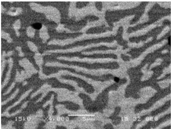
The Cahn-Hilliard equations were first derived at the end of the 50s to model spinodal decom-position and coarsening of metallic alloys during quenching (seeCahn and Hilliard(1958);Cahn (1961)). During cooling of a metallic alloy, the originally stable uniform composition becomes unstable. This leads to phase separation and to the appearance of complex patterns in which domains having different chemical composition can be recognised (see Figure1.1).

The spinodal decomposition differs significantly from phase transitions involving nucleation and growth of one phase in another one (e.g., during the cooling and solidification of water into ice). In the latter case, a thermodynamical barrier between the two phases of the continuum involved in the transition has to be overcome. This leads to phase transitions starting in a

1.1. MOTIVATION—THE MODEL H 7

Figure 1.1: The microstructure of a steel alloy after quenching.

very localised portion of the material (selected by stochastic fluctuations) and then invading all the domain. Pertinent models for these phenomena can be found in the literature devoted to free-boundary problems (seeMeirmanov(1992);Visintin(1996)).

On the other hand, spinodal decomposition is not associated with nucleation phenomena, but to a transition happening throughout the domain as soon as the homogeneous composition state becomes thermodynamically unstable. This instability is seen to occour as soon as the temperature of the mixture θ falls below a critical temperature θc. The microscopic explanation

of the phase separation phenomena observed during spinodal decomposition is to be found in diffusion mechanisms of the different constituents of the mixture, which fails to lead to a stable uniform composition for temperatures below the critical one.

In the mathematical model proposed by Cahn and Hilliard, spinodal decomposition of a binary allow is modeled through a single order parameter field ψ representing the difference of the relative concentrations of the two chemical species involved in the phase separation. Physically relevant values for ψ thus belong to the intervalr´1, 1s. A temperature dependent potential energy F pψq can then be introduced. In order to consistently describe the physical situation just introduced, F is assumed to be a temperature-dependent quadratic perturbation of a super-quadratic convex function F0 so that for θă θc global convexity is lost:

Fpψq “ F0pψq `

θ´ θc

2 ψ

2

Moreover, an energy functional is associated to the configuration of the order parameter field accounting for both the phase separation and the “energetic cost” of the mixing regions. This

8 CHAPTER 1. TWO PHASE FLUID FLOWS

leads to the following assumption

EPpψq “ ε 2 ż Ω |∇ψpxq|2_dx`1 ε ż Ω Fpψpxqq dx. (1.1.1)

Here, the first term penalises the size of the transition areas between the different domains of (almost) pure composition, while, for under-critical temperatures, the second favours the phase separation between the two constituents. The parameter ε appearing in this last expression is seen to be related with the thickness (9?ε) of the transition region between different phases.

Having introduced an energy for the order parameter field, the next step consists in the derivation of an associated evolution equation describing spinodal decomposition. This goal can be achieved by considering a gradient flow approach in a suitable Hilbert space. Choosing as ambient spacepH1_pΩqq˚ _{(see Section 1.4below for the notation generally used in this part), the}

resulting system of partial differential equations is $ ’ & ’ % Btψ“ ´∇ · pM∇µq µ_{“ ´ε∆ψ `} 1 εf1pψq. (1.1.2)

Here, the variable µ is usually called chemical potential, while the quantity M is known as mobility and will be kept positive and constant for all the extent of this work (see Cahn et al.(1996); Elliott and Garcke(1996) for an account of the physical relevance of degenerate mobilities). This system is usually supplemented with homogeneous Neumann boundary conditions both on the order parameter field ψ and on the chemical potential µ.

Bnψ“ Bnµ“ 0.

The boundary condition on ψ corresponds to the physically relevant case of no-flux boundary conditions leading to the conservation of the mean composition of the mixture

ż Ω ψptq, dx “ ż Ω ψpt0q dx,

while the assumption on the chemical potential is consistent with the observation that isolines of equilibrium solutions are orthogonal to domain boundaries.

One of the major challenges associated with the Cahn-Hilliard equation is given by the an-alytical form of the potential F . The derivation of the model from thermodynamical principles leads to a singular expression for the potential Fpψq, being bounded, but defined only on the intervalr´1, 1s (seeCahn(1961)):

Fpψq “ θ

2pp1 ` ψq lnp1 ` ψq ` p1 ´ ψq lnp1 ´ ψqq ´ θc

2ψ

2_{. (1.1.3)}

However, the associated potential term fpψq appearing in (1.1.2) is not bounded thus leading to some difficulties in the theory of the well-posedness and asymptotic behaviour of the Cahn-Hilliard

1.1. MOTIVATION—THE MODEL H 9

system. A popular alternative to (1.1.3) is given by regular potentials of the form

F_{pψq “ ψ}p_{´ ψ}2, with pą 2 (and often p “ 4).

These double-well smooth potentials are qualitatively similar to the theoretically relevant singular potential introduced above featuring two symmetric minima separated by an energy barrier. However, they lead to a much simpler well-posedness theory based exclusively on compactness methods (see, e.g.,Lions(1969) for a general introduction to these techniques). Moreover, smooth potentials are much easier to implement in numerical simulations (see the seminal paperElliott and French(1987) as well as the references in Cherfils et al.(2011)). However, being the Cahn-Hilliard equation a fourth order evolution equation, no comparison principle is available and hence, when using smooth potentials, no guarantee is given that the solution will remain in the physically significant interval r´1, 1s. Indeed, in simulations it is observed that this is not the case. This justifies the interest in precise information on the behaviour of solution for smooth potentials approximating the regular ones. This issue will be partially addressed in Chapter 3

(see alsoFrigeri and Grasselli(2012b,a)).

Finally, another important open problem associated with the singular potential F is the so called “separation from pure phases property”. Indeed, for solutions of the Cahn-Hilliard equation on bounded domains in R2_{, it can be seen that after a sufficiently long time (which is however}

uniform with respect to the norm of the initial data) the order parameter field ψ is uniformly separated from the pure phases 1 and´1 (seeMiranville and Zelik(2004)). This property is still unknown in the three-dimensional case and the techniques used in its proof do not seem to be carried over in a physically significant way to the full model H. We refer the interested reader toCherfils et al.(2011) for a recent thorough review of the mathematical theory associate to the Cahn-Hilliard equation.

1.1.2

On the Navier-Stokes equations

In order to describe the flow of an incompressible fluid, one of the best known models is given by Navier-Stokes equations. These model linear viscous fluids where the stress tensor σ linearly depends on the (symmetric part of) velocity gradient Du through a relation of the form

τ “ ´πI ` 2νDu. (1.1.4)

Here and in the following, the velocity of the fluid will be denoted by u, while π will be the isotropic component of the stress (pressure) and ν the viscosity coefficient. This gives rise to the

10 CHAPTER 1. TWO PHASE FLUID FLOWS

following system of partial differential equations $ ’ & ’ % Btu` pu · ∇qu ´ ν∆u “ ∇π ` g ∇_{· u“ 0.} (1.1.5)

Natural boundary conditions are given by the no-slip boundary conditions

u_{“ 0}

Although the Navier-Stokes equations are among the most studied equations of mathematical physics (seeTemam(1984) for an thorough introduction), very little has been discovered on their well-posedness after the seminal work of Leray in the 30’s (seeLeray(1934)). The situation, as known today for bounded domains, is as follows

2D case In this case, the Navier-Stokes equations are well posed in the Hadamard sense. By this we mean that for square integrable initial data and forcig term g, there exists a unique weak solution, which depends continuously on these data. Moreover, for more regular initial conditions, also strong solutions can be constructed and these are unique as well.

3D case On bounded domains in R3_{, equation (1.1.5) admits a weak solution starting from}

square-integrable initial data. However, this solution is not known to be unique. Nonethe-less, one can show the following “strong-weak” uniqueness property: if a strong solution exists (i.e., a solution belonging to L2_{p0, T ; H}2_{pΩqq X Cpr0, T s; H}1_{pΩqq—see Section1.4for}

the notation), then it is unique in the class of weak solutions. The question whether strong solutions exist for any regular (i.e. H1_{pΩq) initial datum remains still unanswered.}

For a thorough introduction to the mathematical theory of Navier Stokes equations, we refer the interested reader to the monographsTemam(1984,1995).

1.1.3

Coupling Cahn-Hilliard and Navier-Stokes models

Having briefly reviewed the Cahn-Hilliard and the Navier-Stokes equations, we can now introduce the system of partial differential equations resulting from the physical description of a binary fluid. As stated before, we will discuss the so called model H, which can also be seen as arising from the coupling of the two models just discussed. This model has been rigourously derived in the works by Gurtin et al. Gurtin et al.(1996), by Hohenberg and HalperinHohenberg and Halperin (1977) and, more recently, in the works by MorroMorro(2010) and HeidaHeida et al. (2012). One of the fundamental assumptions in its derivation is that both constituents have the same density (seeAbels (2009b) for the “unmatched densities” case).

1.1. MOTIVATION—THE MODEL H 11

The resulting system, which will be the object of investigation in the next four chapters is $ ’ ’ ’ ’ ’ ’ ’ ’ & ’ ’ ’ ’ ’ ’ ’ ’ % Btu` pu · ∇qu “ ´∇π ` ∇ · pτ pDu, ψqq ´ ε∇ · p∇ψ b ∇ψq ` gptq ∇<sub>· u“ 0</sub> Btψ` pu · ∇qψ “ ∇ · pM∇µq µ“ ε´1_f1_{pψq ´ ε∆ψ.} (1.1.6)

We use here a notation consistent to the one described for the Cahn-Hilliard and the Navier-Stokes equation earlier in this section. However, we emphasise the exact meaning, which has to be given to the velocity u in this setting. In principle, one can assume that a velocity can be assigned to each fluid constituting the mixture (and, indeed, this can be done in the derivation of the model from basic principles of continuum mechanics). In the case of “matched densities” fluids considered here, u is the averaged velocity of the two constituents of the mixture. We also observe that in system (1.1.6) the coupling between the Navier-Stokes equations and the Cahn-Hilliard equation occours in three places:

• in the additional convective termpu · ∇qψ appearing in the evolution equation for the order parameter field (cf. equation (1.1.2));

• in the Korteweg force ∇ ·p∇ψ b ∇ψq giving rise to an additional bulk force in the Navier Stokes equations. We note that, up to a gradient term (which can however be easily reab-sorbed in the pressure π), this term can also be conveniently written as µ∇ψ or as ´ψ∇µ; • in the viscous term of the momentum equation in the form of an order-parameter-dependent

viscosity τ “ νpψq∇u (cf. equation (1.1.5)).

Finally, system (1.1.6) is usually supplemented by no-slip boundary conditions on the velocity field and by no-flux boundary conditions on the order-parameter field and chemical potential:

u_{“ 0, B}nψ“ 0, Bnµ“ 0, onBΩ. (1.1.7)

and by a given initial datum

u_{p0q “ u}0, ψp0q “ ψ0, in Ω.

In the case of Newtonian fluids (i.e. for τpDuq“ 2νDu), the well-posedness of the model H. (also referred to as Cahn-Hilliar-Navier-Stokes system—CHNS—in the following) has been widely investigated in the literature (see also Liu and Shen (2003) for contributions to a very similar model). As can be easily expected from our preliminary discussion of the Cahn-Hilliard and Navier-Stokes equations, when discussing existence results for the model H, the space dimension

12 CHAPTER 1. TWO PHASE FLUID FLOWS

and the hypothesis on the double-well potential play a crucial role. System (1.1.6)–(1.1.7) has been firstly studied inStarovoitov (1997) for Ω“ R2 _{and regular potential. Then, in the case}

of bounded domains in R2 _{and for non-constant viscosity ν “ νpψq, global existence results for}

both weak and strong solutions were obtained in Boyer (1999) (see also Boyer (2001) as well as Abels and Feireisl (2008) for the compressible case). More recently, the case of logarithmic potentials has been considered inAbels (2009b) (see also Abels (2009a)), where, in the absence of non-gradient external forces, the convergence of solutions to a single equilibrium has been established. This issue has also been investigated inZhao et al.(2009) for smooth potentials. A further related contribution (seeAbels(2009b)) proves the existence of a (weak) global attractor (which is strong in dimension two—see Section1.3for pertinent definitions). A rather complete picture of the longtime behavior in the case of bounded domain in R2 _{can be found in Gal and} Grasselli (2010a). Finally, in the case of 3D bounded domains and assuming time-dependent external forces, existence of trajectory attractors has been demonstrated in Gal and Grasselli (2010b).

Essentially, in all the above contributions to this field, the well-posedness results obtained for the model H are equivalent to those known for the uncoupled Navier-Stokes equations. In particular well-posedness in the Hadamard sense is obtained in the case of bounded domains in R2_{, while only partial information as described in Section1.1.2above is available in the case of}

bounded domain in R3_.

The effectiveness of model H for numerical simulations has also been widely assessed. We refer the interested reader to, among others,Badalassi et al.(2003);Kay et al.(2008);Kim et al. (2004);Shen and Yang(2010) and references therein.

1.2

Some generalisations of the model H

Having reviewed the standard model H, we now introduce some of its generalisations that will be discussed in the present work. These essentially involve two terms appearing in (1.1.6): mod-ifications in the viscosity term ∇ · τ with respect to the linear assumption (1.1.4) lead to the so called non-Newtonian fluid models; changes in the description of the interaction between the constituents of the mixture, may lead to chemically reacting and/or non-local interactions. We will briefly discuss these phenomena in this section.

1.2.1

Non-newtonian fluids

The so-called Ladyzhenskaya model for non-Newtonian fluids was proposed in the 60’s (see La-dyzhenskaya(1967)) both on physical and mathematical grounds. Through the introduction of

1.2. SOME GENERALISATIONS OF THE MODEL H 13

a suitable non-linearity in the stress-velocity gradient relation, both shear-thinning (as lava or blood) and shear-thickening fluids (like cornstarch–water mixtures or soaked sand) can be effec-tively modeled. These materials exhibit smaller and smaller (respeceffec-tively greater and greater) resistance to motion as the gradient of the deformation rate becomes larger. In particular, for binary fluid flows, the following non-linear constitutive relation for the fluid may be assumed

τpDu, ψq“. `ν1pψq ` ν2pψq|Du|p´2

˘

Du (1.2.1)

where ν1and ν2are suitable positive and sufficiently smooth functions and where the exponent p

is assumed to be larger than 1. The case pă 2 corresponds to a concave relation between stress and velocity gradient and can model shear thinning fluids. On the contrary, for p ą 2, τ is a convex function of Du and therefore, shear-thickening fluids are described. In the case p“ 2 the standard Navier-Stokes equations are recovered.

Concerning the mathematical theory of single component Ladyzhenskaya fluids, many inter-esting results have been obtained in recent years (see Feireisl and Pražák (2010) for a recent review on the subject). In particular, focusing on the case of bounded domains of R3 _{and for}

shear-thickening fluids, it has been shown that full well-posedness in the Hadamard sense can be recovered. This is in contrast to what happens for the standard Navier-Stokes equations. Indeed, in the regime pą 11

5, existence and uniqueness of weak solutions can be proven for the system

$ ’ & ’ % Btu` pu · ∇qu “ ´∇π ` ∇ · pτ pDuqq ` g ∇· u“ 0

with homogeneous Dirichlet boundary conditions u“ 0 (seeLadyzhenskaya(1967);Lions(1969). The key point for obtaining these enhanced well-posedness results lies in a change of the functional setting where solutions are searched: instead of the usual weak regularity L2_pH1

0,divpΩqq, one

can now look for weak solutions belonging to Lp_pW1,p

0,divpΩqq (see Section 1.4 for the notation

used here). This allows testing the equation against a solution obtained through any suitable approximation method (or through monotonicity arguments, like inLions(1969)) thus deducing energy identities for the solution as well as suitable continuous dependence estimates.

Concerning the system arising from (1.1.6) with (1.2.1) (which may be called Ladyzhenskaya-Cahn-Hilliard—or LCH—system), some results are already available in the literature. In par-ticular, the case of a regular double well potential F has been studied in Kim et al.(2006) and well-posedness results obtained, that are analogous to those just discussed in the case of a single fluid. A complete overview of the regular case can be found in Grasselli and Pražák (2011), where also the large-time behaviour of the system is studied and the existence of global as well as exponential attractors proven (see Section1.3below).

14 CHAPTER 1. TWO PHASE FLUID FLOWS

One could expect the situation to be similar also in the case of singular potentials. However, as we shall see in Chapter2, for the LCH system with singular (i.e., logarithmic) potential a complete well-posedness theory seems to be out-of-reach. This is due to the worsening in the time regularity of the velocity field when p becomes larger (see the Remark2.5.1). In particular we will discuss existence results as well as a characterisation of the large-time behaviour of solutions through trajectory attractors (see Section1.3below).

1.2.2

Oono reaction term

The model H can also be suitably modified to account for possible transitions between the two components of the mixture. This is particularly relevant in the case of chemically reacting fluid flows (seeHuo et al.(2003,2004);Teramoto and Nishiura(2002);Villain-Guillot(2010)). Usually, the corresponding modified Cahn-Hilliard equation for describing the phase separation process in the presence of chemical reaction is known as the Cahn-Hilliard-Oono equation—CHO—seeOono and Puri(1987). Moreover, such an equation also arises in slightly different contexts (e.g., phase separation in diblock polymers) with other names (see, for instance, Aristotelous et al.(2012); Choksi et al.(2011) and references therein). In particular, the resulting CHO system is

$ ’ & ’ % Btψ` ǫpψ ´ c0q “ ´∇ · pM∇µq µ“ ´ε∆ψ `1 εf1pψq. (1.2.2)

where ǫ is proportional to the reaction rate and c0is the thermodynamical equilibrium composition

of the mixture considered. As for the boundary conditions, the usual no-flux boundary conditions used in the Cahn-Hilliard equation can be retained also in this case.

Several features distinguish the solutions of the usual Cahn-Hilliard equation from those of the CHO system. First, the equilibria of the CHO equation display some clear periodic patter, such as dots or lamellæ according to the relative equilibrium concentration of the constituents (see Figure1.2). Secondly, the mean composition of the mixture is not fixed by the initial condition (as happens, e.g., for an alloy), but changes with time converging to the prescribed thermodynamical equilibrium c0 (see equation (1.2.4) for the analogous result for the full variation on the model H

below).

Coupling the CHO system with the Navier-Stokes equations and proceeding exactly as in the derivation of the model H, one obtains the following system of Partial differential equations

1.2. SOME GENERALISATIONS OF THE MODEL H 15

Figure 1.2: Pattern formation in a mixture of diblock copolimers. Observe the regular dotted regions and the lamellæ appearing as a consequence of small local fluctuations of the mean composition of the mixture. Compare with the pattern arising in alloys (see Figure1.1).

usually called the Navier-Stokes-Cahn-Hilliard-Oono system (or NSCHO system, for short) $ ’ ’ ’ ’ ’ ’ ’ ’ & ’ ’ ’ ’ ’ ’ ’ ’ % Btu` pu · ∇qu ´ ∇ · pνpψqDuq “ ∇π ` µ∇ψ ∇· u“ 0 Btψ` pu · ∇qψ ` ǫpψ ´ c0q “ ∆µ µ_{“ ´∆ψ ` fpψq.} (1.2.3)

This system can be supplemented by the same boundary conditions used for the model H itself (see (1.1.7)).

As anticipated above for the simpler CHO system, an important feature of the NSCHO model concerns the evolution of the mean composition of the mixture. Indeed, integrating the third equation in (1.2.3) over the domain Ω and taking (1.1.7) into account, we obtain the following evolution equation for the (spatial) averagexψy

Btxψy ` ǫpxψy ´ c0q “ 0,

from which we deduce

xψy ptq “ c0` e´ǫtpxψ0y ´ c0q. (1.2.4)

Hence, ifxψ0y “ c0, then the total mass is conserved as in the classical Cahn-Hilliard equation.

Otherwise, we are in the off-critical mixture case, i.e. the order parameter average at steady state differs fromxψ0y (cf. Huo et al.(2003) where numerical simulations are performed in 2D by taking

16 CHAPTER 1. TWO PHASE FLUID FLOWS

periodic boundary conditions). This feature leads to interesting problems for the description of the long-term behaviour of solutions.

In Chapter 4, we will study the well-posedness as well as robustness of the asymptotic be-haviour of solution with respect to the parameter ǫ.

1.2.3

Non-local models

The Cahn-Hilliard equation derived from the potential energy (1.1.1) implicitly assumes that the interactions between the components of the mixture are short-ranged (i.e., local). However, we may also assume that the interaction energy between two particle of the mixture at points x and yis given by a Kac potential of the form

γnK_{pγ|x ´ y|q} with γą 0.

In this case, a statistical mechanical derivation of the model leads to the following non-local total energy for the system (seeGiacomin and Lebowitz(1997,1998))

EPpψq “ ε 2 ż Ω ż Ω

K_{p|x ´ y|q|ψpxq ´ ψpyq|}2_dxdy

` ε ż Ω ż Ω K<sub>p|x ´ y|qψpxqp1 ´ ψpxqq dxdy `</sub> 1 ε ż Ω F_{pψpxqq dx.} The resulting Cahn-Hilliard equation is then given by

$ ’ & ’ % Btψ“ ´∇ · pM∇µq µ“ εaψ ´ εK ˚ ψ `1 εf1pψq. where apxq is defined by apxq“. ż Ω Kp|x ´ y|q dy

and where ˚ denotes the convolution operator. In the case of smooth interaction kernels K, this system has been studied inGajewski and Zacharias(2003);Bates and Han(2005). We also note that the non-local model can be reduced to the classical local one by suitably rescaling the interaction kernel K so that its mass is concentrated around the origin.

An interesting problem related to this non-local formulation of the Cahn-Hilliard equations is given by its effects on the properties of the full model H when it is substituted to the local Cahn-Hilliard one. In the case of regular interaction kernels, this issue has recently been addressed in a series of research papers (seeColli et al.(2012);Frigeri and Grasselli(2012a,b)). In particular, in these papers, well-posedness results have been obtained and a description of the asymptotic behaviour of the system has been given.

1.3. LARGE-TIME BEHAVIOUR FOR SOLUTIONS OF PARABOLIC SYSTEMS 17

However, not only regular kernels can be studied, but also singular ones are of great interest for applications. This choice leads to operators somehow similar to the so-called s-Laplacian, although defined on bounded domains (seeSilvestre(2007) for an introduction to these operators on the whole space). We will give some preliminary results on the well-posedness of the Cahn-Hilliard equation with non-local interactions described by a singular kernel in Chapter5. These have to be considered a preliminar work towards the study of the full nonlocal model H with singular kernels.

1.3

Large-time behaviour for solutions of parabolic systems

We now wish to review some of the theory of (infinite dimensional) dynamical system introducing the tools that will be used to describe the large-time behaviour of solutions to evolution equations. We refer the interested reader to the monographs Temam (1997);Robinson (2001) for a more comprehensive introduction to the subject (see also the reviewMiranville and Zelik(2008)). After briefly recalling the basic theory of global attractors we shortly discuss some of its generalisations, which are needed to study the behaviour exhibited by evolution equations arising in examples of practical interest. In order not to break the exposition into pieces, we refer to Section 1.4for a detailed description of the notation used in this section and in the remaining of this part of the present manuscript.

1.3.1

Short overview of the classical theory of attractors

The theory of attractors for infinite-dimensional dynamical systems was originally developed by Ladyzhenskaya, Vishik and collaborators in the 70s (see Babin and Vishik (1992) for an early account on the subject). For the sake of clarity, we will briefly discuss here only the case of autonomous systems referring to Section1.3.4for the discussion of the pertinent setting for the non-autonomous case (see also Section 3.2 as well as Carvalho et al.(2013) and the references therein).

The starting point of the theory of (global) attractors is an abstract reinterpretation of the structure of the solutions of an evolution equations through the notion of (possibly non-linear) semigroup.

Definition 1.3.1. Let H be a metric. A family of operatorstSptqutPR` s.t. Sptq: H Ñ H for all

tě 0 is called semigroup if the following properties hold • Sp0q “ I

18 CHAPTER 1. TWO PHASE FLUID FLOWS

The variable t is usually calledtime.

Remark 1.3.1. For the purposes of this work we will always assume that H is an Hilbert or a Banach space.

One of the main goals of the contemporary theory of dynamical systems is to prove significant properties on the solutions of an evolution equation after large time. Among many others, natural question are whether the solutions eventually regularise (this may also happen after a finite time, e.g., in the case of parabolic systems as those which will be studied in the present work), how complex the asymptotic behaviour of the system can be and how fast this significant regime can be reached (at least from a practical point of view). The theory of (global) attractors for evolution PDEs tries to give an answer to these question by constructing “small” sets in thephase space H, which contain the eventual evolution of the system. Moreover, precious quantitative information may be deduced from the fractal dimension of these sets and from the rate at which they attract all other physically possible initial data.

From the abstract semigroup description just introduced, the answers to the above questions can be translated in simple properties of the semigroup in the phase space. In particular, reg-ularising properties are epitomised in the requirement that there exists a compact subset of H which absorbs all solutions in the sense made precise by the following definition.

Definition 1.3.2. LettSptqutPR` be a semigroup on a metric space H. A subset B isabsorbing

for the semigroup tSptqutPR` if for all bounded sets U Ă H, there exists a time t “ tpBq such

that

SptqU Ă B @t ě t.

In order to describe more precisely (and quantitatively) the behaviour of solutions we will also need to use the metric structure of the phase space H. In particular, we introduce the Hausdorff semi-distance between sets

Definition 1.3.3. Let H be a metric space with distance d : Hˆ H Ñ R. Given two sets A and B theHausdorff semi-distance between A and B is given by

distHpA, Bq“ sup. xPA

inf

yPB

dpx, yq. We can now introduce the main object of interest of this section.

Definition 1.3.4. LettSptqutPR` be a semigroup on a metric space H. The global attractor for

tSptqutPR` is a set AĂ H such that

1.3. LARGE-TIME BEHAVIOUR FOR SOLUTIONS OF PARABOLIC SYSTEMS 19

• A is invariant (i.e. SptqA “ A, for all t ě 0);

• A attracts all bounded subsets BĂ H. By this we mean that lim

tÑ8distHpSptqB, Aq “ 0 for all B Ă H with B bounded.

It is easy to see that, if the (global) attractor exists, then, by invariance, it has to be unique. Loosely speaking, the attractor contains all the “relevant” information for understanding the persistent dynamics of the evolution equation (or semigroup) of interest. To give examples re-lated to the questions introduced before, the complexity of the asymptotic dynamics can be measured through the evaluation of the fractal dimension of the (global) attractor. Moreover, the rate at which solutions approach the asymptotic regime(s) corresponds to the rate at which distHpSptqB, Aq goes to 0.

We only recall the following fundamental existence result for (global) attractors (cf. (Temam, 1997, Theorem 1.1))

Theorem 1.3.1. _{Let tSptqutPR}`be a (non-linear) semigroup acting on a metric space H. Assume

that Sptq is continuous for any t ě 0 and that there exists a compact absorbing set B Ă H. Then, tSptqutPR` has a (compact) global attractor A. Moreover

A_“ č sě0 ď těs SptqBH holds.

1.3.2

Trajectory attractors

The simple picture of global attractors just introduced, although appealing, cannot in general be used as it is to deal with the solution semigroups arising from applications. Without any attempt of completeness, we would now like to bring to the attention of the reader some of its possible extensions and the subjacent reasons for their development. In particular, we will focus on possible cures to the lack of uniqueness (also related to possible issues with the continuity of the semigroup), on the problems related with the rate of decay of solutions towards the attractor itself and on a possible extension of the theory of global attractors to the non-autonomous case. We start here by addressing the issue related to non-uniqueness.

In the case when uniqueness of solutions is not known, a possible approach to the description of the asymptotic behaviour is given by the theory of trajectory attractors developed by Chepyzhov and Vishik (see Chepyzhov and Vishik (2002, 1997)). This theory was introduced to address, among others, the issues related to the lack of information concerning uniqueness of solutions for the Navier-Stokes equations on 3D domains. The key ingredient of this approach is a different