Doppler spectrum segmentation of radar sea clutter by mean-shift and information geometry metric

HAL Id: hal-01536373

https://hal-mines-paristech.archives-ouvertes.fr/hal-01536373

Submitted on 11 Jun 2017

HAL is a multi-disciplinary open access archive for the deposit and dissemination of sci-entific research documents, whether they are pub-lished or not. The documents may come from teaching and research institutions in France or abroad, or from public or private research centers.

L’archive ouverte pluridisciplinaire HAL, est destinée au dépôt et à la diffusion de documents scientifiques de niveau recherche, publiés ou non, émanant des établissements d’enseignement et de recherche français ou étrangers, des laboratoires publics ou privés.

Doppler spectrum segmentation of radar sea clutter by

mean-shift and information geometry metric

Frédéric Barbaresco, Thibault Forget, Emmanuel Chevallier, Jesus Angulo

To cite this version:

Frédéric Barbaresco, Thibault Forget, Emmanuel Chevallier, Jesus Angulo. Doppler spectrum seg-mentation of radar sea clutter by mean-shift and information geometry metric. 17th International Radar Symposium (IRS’16) , May 2016, Krakow, Poland. pp.1 - 6, �10.1109/IRS.2016.7497314�. �hal-01536373�

Doppler Spectrum Segmentation of Radar Sea Clutter

by Mean-Shift and Information Geometry Metric

Frédéric Barbaresco, Thibault Forget Advanced Radar Concepts Business Unit

Thales Air Systems

Voie Pierre-Gilles de Gennes, F91470 Limours, France {frederic.barbaresco,thibault.forget}@thalesgroup.com

Emmanuel Chevallier, Jesus Angulo Department of Mathematics and Systems

Mines ParisTech

35 Rue Saint-Honoré, 77300 Fontainebleau, France {emmanuel.chevallier,jesus.angulo}@mines-paritech.fr Abstract— Radar sea clutter inhomogeneity in range is

characterized by Doppler mean and spectrum width variations. We propose a new approach for robust statistical density estimation and segmentation of sea clutter Doppler spectrum. In each range cell, Doppler is characterized by a Toeplitz Hermitian Positive Definite covariance matrix that is coded in Poincaré’s unit poly-disk and we use adaptation of standard kernel methods to density estimation on this specific Riemannian manifold. Based on this non-parametric approach to estimate statistical density of Doppler Spectrum, we address the problem of sea clutter data mapping and segmentation by extending “Mean-Shift” tool for these densities on Poincaré’s unit poly-disk. This statistical segmentation is requested for robust detection of targets in sea clutter, especially in case of high sea state.

Index Terms—Sea Clutter; Fisher Metric; Information

Geometry; Kernel Density Estimation; Mean-Shift Algorithm

I. INHOMOGENEOUS DOPPLER SPECTRUM OF SEA CLUTTER

We are studying highly variable Doppler spectrum characteristics that occur in the littoral sea clutter environment, to improve robustness of adaptive coherent CFAR detector.

Doppler that is observed varies from 0 to 5 m/s and peaks at more than 10 m/s induced by breaking waves. The coastal circulation has local characteristics and is very variable depending on weather conditions. Close to the shore, we have to take into account drift currents. The permanent and seasonal components constitute the so-called general currents. These are generally low. The wind generates the drive current drift of the surface layers, which is transmitted by viscosity to the deeper layers. According to the theory, for a wind that had blown in the same direction for several days at any point of a body of water and indefinite water depth (over 200 m), the surface drift current is directed at 45 ° of the wind direction. The decrease of these parameters (duration, extent, depth) has the effect of reducing the deviation. So, near the coast and variable wind, the surface drift current is substantially oriented in the direction of the wind.

The coast is an obstacle for the drift current, causing an accumulation or conversely a water withdrawal, according to the relative orientation of the wind and of the coastline. Tidal currents are often distinguished by their very high speed. They can indeed be greater than 10 knots (5 m/s). Usually the directions of the tide vary very quickly. The variation of the current amplitude with the amplitude of the wave is not equal if

the tide behaves like a wave, a standing wave or an hydraulic phenomenon of filling/emptying a basin. In figure 1, we give the surface currents in knots from the SHOM close to Ouessant Island. Variations can therefore be seen from 0 to 4 m/s.

Figure 1. Maximum current in knots in French Brittany close to the Shore

IFREMER has developed the accurate Mars model (coastal hydrodynamic model) as illustrated in the figure 2:

Figure 2. Residual streams in m2_{/s (speed x water level) for different}

exposure to winds, illustrating the spatial variability of the current.

As consequence, Doppler mean is not zero and varies along the range axis, induced by means of Doppler surface current (which may vary depending on the distance to the coast and wind exposure). These variations may be important and equal to several meters per second (tidal current and the case of variable wind exposure in the presence of island or local phenomena depending on the water depth). The spectral width of the sea clutter may also vary along the distance axis based on the variable swell after exposure to wind. Simulation of coherent radar sea clutter has been described in [20,21,22,23]. For the Ground Clutter of the Shore, the Doppler spectrum width could vary with vegetation and wind exposure.

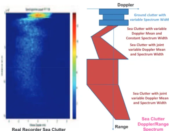
We illustrate in the figure 3, Doppler variations of clutter in littoral environment.

Doppler

Range Real Recorder Sea Clutter

Sea Clutter Doppler/Range

Spectrum

Sea Clutter with variable Doppler Mean and Constant Spectrum Width

Sea Clutter with joint variable Doppler Mean and Spectrum Width

Sea Clutter with joint variable Doppler Mean and Spectrum Width Ground clutter with variable Spectrum Width

Figure 3. (left) Recorded Doppler/Range Spectrum in coastal environment,

(right) synthetic model of Doppler Mean/Width variations

On real sea clutter recorded in the figure 4, we can observe evolution of Doppler/Range Spectrum for different Sea states 1, 3 and 5.

Figure 4. Recorded Doppler/Range Spectrum in coastal environment for different Sea states: 1 (left), 3 (middle), and 5 (right)

II. ROBUST STATISTICAL DENSITY ESTIMATION OF SEA

CLUTTER DOPPLER SPECTRUM

A. Median Estimation of Doppler Spectrum Statistics based on Fréchet Barycenter and Information Geometry

Classical methods for estimation of Mean Clutter Doppler spectrum are based on Multi-segment Burg or “Fixed Point” algorithms using a sliding window along range axis. Unfortunately, these approaches suffer of many drawbacks in case of non-stationary clutter.

Doppler Doppler

Range

Multisegment Burg or Fixed Point Algorithms

Median Burg Spectrum (Geometric geodesic

barycenter)

Doppler Doppler

Range

Figure 5. Comparison of classical methods (Multi-segment Burg or Fixed Point) with geodesic median L1-barycenter in case of (left) Doppler Mean

variation, (right) Doppler spectrum width variation

Both methods will estimate the covariance matrix that will optimize the whitening for all cells of the learning window. If the Doppler mean or spectrum width varies in range along radar cells of the learning window, the estimated spectrum will be widened and will be no longer representative of the local spectrum. As first approach to mitigate this drawback, we propose to compute “Median” Doppler spectrum as L1 geometric barycenter. The covariance matrix will be estimated to minimize the sum of geodesic distance to each covariance matrix of learning window radar cells. This robust approach will interpolate a Doppler spectrum as illustrated in the 2 cases of Doppler variations in the figure 5.

In the figure 6, we illustrate the good property of geodesic median L1-barycenter method to estimate Doppler Spectrum in case of non-stationary for clutter Doppler mean.

Figure 6. Doppler Mean variation: (left) Estimation by classical methods, (right) Estimation by geodesic median L1-barycenter method

As illustrated in the figure 6, as “Fixed Point” and Multi-segment Burg algorithms take into account all neighbor cases with the same weights, the resulting spectrum is artificially widened. On the contrary, the median-based estimator only depends on the considered Riemannian geometry in the space of covariance matrices, and is able to “interpolate” Doppler spectrum to provide a good estimator of “centrality”.

For the robust metric and distance requested to define geodesic median L1-barycenter, we propose to use Fisher metric. As the signal is assumed to be stationary in each burst of radar cells, we can apply the Trench theorem proving that THPD (Toeplitz Hermitian Positive Definite) Covariance matrix could be parameterized by Complex Auto-Regressive

(CAR) model. All THPD matrices are diffeomorphic to (P0,

μ1,…, μn)∈R+xDn (P0 is a real “scale” parameter, μk are called reflection/Verblunsky coefficients of CAR model in D the complex unit Poincare disk, and are “shape” parameters). This Trench theorem is based on the Block Structure of THPD matrices given by:

» ¼ º « ¬ ª + = ₊ − − − − − − − + − − − − 1 1 1 1 1 1 1 1 1 1 1 n n n n n n n n n n _{A R A A} A R α α α α (1) with

( )

T V V * = + _, 1 0 0=α− P ,

[

]

1 1 2 1 ₁ − − − _{= −} n n n μ α α and

» ¼ º « ¬ ª + » ¼ º « ¬ ª = − −− 1 0 ) ( 1 1 n n n n A A A _μ with V(−)=J.V*and » » » » ¼ º « « « « ¬ ª = 0 0 1 1 0 0 1 0 0 " # $ $ $ # " J (2)

This block structure also provides iteratively André-Louis

Cholesky decomposition of −1 n R :

(

)

− _{=Ω Ω} + = Ω 1 1/2_. 1/2 n n n n n α R with » ¼ º « ¬ ª Ω − = Ω − − + − 2 / 1 1 1 1 2 2 / 1 ₁ 1 0 n n n n n A μ (3)

Complex autoregressive parameters

[

n

]

T

n n n a a A () () 1 " = and reflections coefficients

_{{ }}

1 1 − = N i i

μ are computed by Regularized

Burg algorithm from pulses

_{{ }}

N

k

k

z( ) =1of each radar burst:

1 and ) ( . 1 , 1 , ) ( ) ( ) ( f (0) 0 1 2 0 0 0 = = =

¦

= = a k z N P ,...,N k= k z k b k N k (4) ¯ ® ­ + − = − + = ° ¯ ° ® ­ = + = = − = + − + − + − − − = = − − − − − − − + = − = − − − + = − = − − − − −

¦

¦

¦

¦

) ( . ) 1 ( ) ( ) 1 ( . ) ( ) ( , . 1 1 1 ) ( ) 2 ( with . . 2 ) 1 ( ) ( 1 . . . 2 ) 1 ( ). ( 2 1 1 1 * 1 1 1 ) ( * ) 1 ( ) 1 ( ) ( ) ( 0 2 2 ) ( 1 1 0 2 ) 1 ( ) ( 2 1 2 1 1 1 1 ) 1 ( ) 1 ( ) ( * 1 1 k f k b k b k b k f k f a a a a a to n-For k= n k a k b k f n N a a k b k f n N to N-For n n n n n n n n n n n n n k n n n k n k n n k N n k n k n k n k n n N n k n k n k n n k n k n n n μ μ μ μ π γ β β β μ (5)

In the framework of Information Geometry, we can consider this covariance matrix as a parameter for a probability density

of a multivariate random process of zero mean p(./θ). The

fisher metric I(_{θ) defines a Riemannian metric in the space of}

parameters:

(

) (

)

[

+

]

= =

¦

= + j i ij i j d d g d I d d Z p Z p KL ds , * 2 _{/θ, /θ θ θ (θ) θ θ θ} (6) With

_{[ ]}

» » ¼ º « « ¬ ª ∂ ∂ ∂ − = = * 2 , ) / ( log ) ( j i j i ij Z p E I g θ θ θ θ (7)

For Exponential families, the Entropy is given by ) ( , ) (θ = θ θ −Φθ S withlogp_θ(_ξ)=−_θ,_ξ +Φ(_θ), _θ =E(_θ) ,

[ ]

* 2 , ) ( ) ( j i j i I θ θ θ θ ∂ ∂ Φ ∂ − = and 1 * 2 * 2 _{( ) ( )} − » » ¼ º « « ¬ ª ∂ ∂ Φ ∂ = » » ¼ º « « ¬ ª ∂ ∂ ∂ j i j i S θ θ θ θ θ θ (8)

We can then define a metric in dual space of θ =E(θ):

* 2 , * 2 _with ( ) j i dual ij j i j i dual ij dual S g d d g ds θ θ θ θ θ ∂ ∂ ∂ = =

¦

(9)

For Multivariate Gaussian Process of zero mean, Entropy is

(

det

)

log( . ) log ) (_{R R} 1 _e S n = n− − π , developed by use of (1):

[

]

[

0

]

1 1 2 . . log 1 log ) ( ) (R n k n eP S n k k n =−

¦

− −μ − π − = (10)

If we use the canonical vector of parameters:

[

]

[

[

]

T

]

n T n n _{P E P} 1 1 0 1 1 0 ) ( − − = = μ μ μ μ θ " ! (11)

The dual metric of Information Geometry is finally given by:

(

)

¦

¦

− = − − + ¸¸ ¹ · ¨¨ © § = = 1 1 2 2 2 0 0 , * ) ( ) ( 2 1 ) ( . n i _i i j i n j n i dual ij dual d i n P P d n d d g ds μ μ θ θ (12)

The robust “Information Geometry” distance can be computed

by integration in product space R+_xDn _:

{ }

(

)

(

{ }

)

[

]

¦

−

(

)

= − = − = ¸¸ ¹ · ¨ ¨ © § ¸¸ ¹ · ¨¨ © § − + − + ¸ ¸ ¹ · ¨ ¨ © § = 1 1 2 1 , 0 2 , 0 2 1 1 2 , 2 , 0 1 1 1 , 1 , 0 2 1 1 log 2 1 log , , , N i i i N i i N i i _P N i P N P P d δ δ μ μ with * 2 , 1 , 2 , 1 , 1 _{i i} i i i μ μ μ μ δ − − = (13)

The Lp-barycenter on M cells is given by [14, 10, 15,16]:

{

}

(

)

{ }

¦

=

[

(

{

}

)

(

{ }

)

]

− = − = − = − = = M k N i k i k N i barycenter i barycenter p P N i barycenter i barycenter P P d ArgMin P N i median i median 1 1 1 , , 0 1 1 , , 0 , 1 1 , , 0 , , , , 1 1 , , 0 μ μ μ μ (14)

B. Kernel Density Estimation of Doppler Spectrum Statistics In this section, we introduce a kernel density estimation on the elements of the product (P0, _μ1,…, μn)∈R+xDn, to estimate density for Doppler Spectrum. The specificity of the hyperbolic space enables to adapt the different density estimation methods at a reasonable cost. Recently convergence rates for the kernel density estimation without the compact assumption have been introduced, which enables the use of Gaussian-type kernels.

Let _{K :R}+_{→ R}+ _{be a map which verifies the following}

properties:

( )

. =1 ,

_³

.

( )

. =0 , ( >1)=0 ,

(

)

=0

³

K x dx xK x dx K x Sup K(x) n n _R R (15)

Given a point p∈H_n(the hyperbolic space of dimension n;

H2=D), the exponential map exp_pdefines a new injective

parametrization of H_n. The Lebesgue measure of the tangent

space is noted Leb_p. The function _{H → R}+

n p: θ defined by: ) ( ) ( exp ) ( : _* q Leb d dvol q q p p p p →θ = θ (16)

is the density of the Riemannian measure with respect to the

image of the Lebesgue measure of T_pH_n by expp. Given K and

a scaling parameter Ȝ, the estimator of f proposed by Pelletier

[3] is defined by:

_¦

_¸ ¹ · ¨ © § = i i x n k x x d K x k f i λ θ λ ) , ( ) ( 1 1 1 ˆ (17)

Given _pref∈Hn, _μk the empirical measure and “*” the natural

convolution on homogeneous spaces [26], let: ¸¸ ¹ · ¨¨ © § = λ θ λ ) , ( ) ( 1 1 ) ( ~ d p q K q k q K ref p n ref then fk k K ~ * ˆ _=μ (18)

One still needs to obtain an explicit expression of _θp. Given a reference point p, the point of polar coordinates (r, Į) of the

hyperbolic space H_nis defined as the point at distance r of p on

the geodesic with initial direction _α∈Sn−1_{. Since}

n

H is isotropic

the expression the length element in polar coordinates depends only on r. Expressed in polar coordinates the hyperbolic metric

expression is: sinh( ) . 1

2 2 − + = n n S H dr r g g (19)

The polar coordinates are a polar expression of the exponential map at p. In an adapted orthonormal basis of the tangent plane the metric takes the following form:

¸ ¸ ¹ · ¨ ¨ © § = −1 2 2 1 ) sinh( 0 0 1 n I r r G (20)

where G is the matrix of the metric and I_n−1is the identity

matrix of size ní1. The volume volume dvol is given by:

) ( exp ) sinh( 1 ) ( exp . * 1 * p p n p p Leb _r r d Leb d G dvol − ¸ ¹ · ¨ © § = = (21)

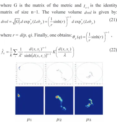
where r = d(p, q). Finally, one obtains: 1_{sinh( )} 1

) ( − ¸ ¹ · ¨ © § = n p r r q θ ,

(

)

¦

¸ ¹ · ¨ © § = − ₋ i i n i n i n k x x d K x x d x x d k f λ λ ) , ( ) , ( sinh ) , ( 1 1 ˆ 1 1 (22)

Figure 7. Estimation of the density for the 3 first reflexion coefficients

III. SEA CLUTTER DOPPLER SPECTRUM MAPPING BASED ON

MEAN-SHIFT ALGORITHM

The original mean shift algorithm is widely applied for nonparametric clustering of data in vector spaces. In this section, we will generalize it to data points lying on Riemannian manifolds of reflection coefficients. This allows us to extend mean shift based clustering to Sea Clutter data mapping for segmentation of area with homogeneous Doppler content. Mean shift is provided by following gradient equation where the _logy(xi) terms lie in the tangent space, and the kernel terms K are scalars. The mean shift vector is a weighted sum of tangent vectors, and is itself a tangent vector. The mean shift iteration is:y_j+₁exp_yj

(

m_λ(y_j)

)

withg(.)=−K'(.) :

) ( log ) , ( ) , ( ) ( 1 1 1 i y n i i n i i _g d y x _x x y d g y m

¦

¦

= − = ¸ ¹ · ¨ © § » ¼ º « ¬ ª ¸ ¹ · ¨ © § = λ λ λ (23)

IV. RESULTS OF MEAN-SHIFT ALGORITHMS ON REAL SEA

CLUTTER DATA

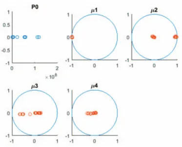
Figure 8 and 9 represent respectively the Doppler spectrum of the radar signal on one burst and its associated reflection coefficients. Figure 10, 11 and 12 show the results obtained after running the Mean-Shift algorithm on the product space

RxD4 _{using different kernel shapes – uniform, quartic and}

Gaussian. The number of samples is 270 along the direction of the radar burst (range axis). It can be seen that the samples tend to converge towards limit points, which represent maxima of the probability density function. There doesn’t seem to be a significant difference coming from the choice of the kernel shape according to the plots obtained.

We can define clusters by specifying a distance threshold to group close points together. The reader must bear in mind that we are reasoning in a product space so this threshold cannot be directly read from the plots.

One solution is to use the convergence criterion used in the

Mean-Shift algorithm (in our case 10-4_{). Then for each point in}

the product space, calculate its distance to the other points and

test whether this distance is lesser than 10-4_{. This way, we can}

define clusters as sets of points which are less than 10-4 _distant

from each other. It is interesting to note that there are less non-convergent point when using the uniform mean-shift (about 2 points) than with the two other kernels (10 to 20 points). Figure 13, 14 and 15 represent the clusters obtained along the range axis. Each color corresponds to one cluster. The x axis does not represent anything. We can see that there are a lot of clusters (35 to 138) with some singletons. It is extremely difficult to interpret these plots in terms of number and width of homogeneous zones due to the lack of smoothness of certain clusters. Next steps would be to investigate different shapes of kernels, using intrinsic smoothing methods such as persistence.

Figure 9. Reflexion coefficients of Sea clutter

Figure 10. Uniform Mean-Shift algorithm run on the product space RxD4

Figure 11. Mean-Shift run with kernel based density estimation (quartic kernels) on the product space RxD4

Figure 12. Mean-Shift run with kernel based density estimation (Gaussian kernels) on the product space RxD4

Figure 14. Clusters obtained from Quartic Mean-Shift (35 clusters)

Figure 15. Clusters obtained from Gaussian Mean Shift (39 clusters)

V. CONCLUSION

We will deepen this non-supervised segmentation method to reduce the number of clusters by using “persistence” approach. This method will be mixed with robust detection algorithm as in [10]. Approach will be also extended for STAP [27].

REFERENCES

[1] E. Arias-Castro, D. Masony and B. Pelletier, On the estimation of the gradient lines of a density and the consistency of the mean-shift algorithm, Journal of Machine Learning Research, 2015

[2] I.M. Loubes and B. Pelletier, A kernel-based classifier on a Riemannian manifold. Statistics and Decisions, Vol. 26, No. 1, pp. 35-51.,2008 [3] B. Pelletier. Kernel density estimation on Riemannian manifolds.

Statistics and Probability letters, Vol. 73, n°3, pp.297-304, 2005

[4] R. Subbarao, P. Meer, Nonlinear Mean Shift over Riemannian Manifolds, Int. Journal of Computer Vision, vol.84, pp. 1–20, 2009 [5] Y. Wanga, X. Huang, L. Wua, Clustering via geometric median shift

over Riemannian manifolds, Information Sciences, Vol. 220, pp.292– 305, Elsevier, 2013

[6] Y.H. Wang, C.Z. Han, PolSAR Image Segmentation by Mean Shift Clustering in the Tensor Space, Acta Aut. Sinica, Vol. 36, No. 6, pp.798-806, June 2010

[7] E. Chevallier, F. Barbaresco and J.Angulo, Probability Density Estimation on the Hyperbolic Space Applied to Radar Processing, GSI’15, Vol. 9389, Springer LCNS, pp 753-761, October 2015

[8] D. M. Asta. Kernel Density Estimation on Symmetric Spaces, Vol. 9389 , GSI’15, Springer LCNS, pp. 779-787, October 2015

[9] J.-Ph. Anker, P. Ostellari. The heat kernel on noncompact symmetric spaces. In Lie groups and symmetric spaces, AMS Trans. Ser. 2, 210, pp.27-46, 2003

[10] A. Decurninge, F. Barbaresco, Robust Burg Estimation of Radar Scatter Matrix for Mixtures of Gaussian Stationary Autoregressive Vectors, submitted to IET UK, http://arxiv.org/abs/1601.02804

[11] A. Decurninge, Univariate and multivariate quantiles, probabilistic and statistical approaches; radar applications, UPMC PhD, March 2015 [12] J.F. Degurse, L. Savy, J.P. Molinie, S. Marcos, A Riemannian Approach

for Training Data Selection in Space-Time Adaptive Processing Applications, Radar Symposium (IRS), Vol. 1, pp.319-324, 2013 [13] E. Chevallier, Morphology, Geometry and Statistics in non-standard

imaging, Mines ParisTech PhD, December 2015

[14] Le Yang, Medians of probability measures in Riemannian manifolds and applications to radar target detection, PhD Thesis, January 2012 [15] M. Arnaudon, F. Barbaresco, Le Yang, Riemannian medians and means

with applications to radar signal processing, IEEE Journal of Selected Topics in Signal Processing, vol.7, n°4, pp. 595-604, 2013

[16] F. Barbaresco, Information Geometry of Covariance Matrix: Cartan-Siegel Homogeneous Bounded Domains, Mostow/Berger Fibration and Fréchet Median, MIG Workshop, Springer, pp. 199–256, 2012 [17] F. Barbaresco F., Koszul Information Geometry and Souriau Geometric,

Temperature / Capacity of Lie Group Thermodynamics, MDPI Entropy, n°16, pp. 4521-4565, August 2014.

[18] F. Barbaresco, Symplectic Structure of Information Geometry: Fisher Metric and Euler-Poincaré Equation of Souriau Lie Group Thermodynamics, GSI’15,Vol.9389, Springer LCNS, pp. 529-540, 2015 [19] A. Aubry & al, Median matrices and their application to radar training

data selection, IET RSN, 2014, Vol. 8, Iss. 4, pp. 265–274

[20] S. Watts, Modelling of coherent detectors in sea clutter, Radar Conference (RadarCon), pp.105-110, May 2015

[21] S. Watts, Modeling and simulation of coherent sea clutter, IEEE Trans AES Vol. 48, No.4, pp. 3033-3317, October 2012,

[22] S. Watts, A new method for the simulation of coherent radar sea clutter, 2011 IEEE Radar Conference RadarCon ‘11, Kansas City, May 2011 [23] V. Corretja, J. Petitjean, J.-M. Quellec, S. Kemkemian, H. Thuilliez, S.

Watts, Sea-spike analysis in high range and Doppler resolution radar data, Radar Conference (Radar), vol., no., pp.1-6, 13-17 Oct. 2014 [24] F. Barbaresco, Super-resolution spectrum analysis regularization: Burg,

Capon & AGO-antagonistic algorithms, EUSIPCO’96, Sept 1996 [25] M. Calvo, J-M.Oller, A distance between elliptical distributions based in

an embedding into the Siegel group, Journal of Computational and Applied Mathematics, n°145, pp. 319-334, 2002

[26] Helgason S. – Geometric Analysis on Symmetric Spaces, Math. Surveys and Monographs, vol. 39,Amer. Math. Soc., Providence, RI, 1994 [27] B. Jeuris, Ben, R. Vandebril, The Kähler mean of block-Toeplitz

matrices with Toeplitz structured blocks, SIAM Journal on Matrix Analysis and Applications, 2nd _{March 2016,}

https://lirias.kuleuven.be/handle/123456789/533797

[28] Information, Entropy and Their Geometric Structures, MDPI Entropy, MDPI AG Basel, Switzerland, A.M. Djafari & F. Barbaresco Editors, 2015, http://books.mdpi.com/pdfview/book/127