HAL Id: hal-01135651
https://hal.archives-ouvertes.fr/hal-01135651
Submitted on 25 Mar 2015
HAL is a multi-disciplinary open access
archive for the deposit and dissemination of
sci-entific research documents, whether they are
pub-lished or not. The documents may come from
teaching and research institutions in France or
abroad, or from public or private research centers.
L’archive ouverte pluridisciplinaire HAL, est
destinée au dépôt et à la diffusion de documents
scientifiques de niveau recherche, publiés ou non,
émanant des établissements d’enseignement et de
recherche français ou étrangers, des laboratoires
publics ou privés.
Distributed under a Creative Commons Attribution| 4.0 International License
Lagrangian concordance is not a symmetric relation
Baptiste Chantraine
To cite this version:
Baptiste Chantraine. Lagrangian concordance is not a symmetric relation. Quantum Topology, 2015,
6 (3), pp.451-474. �hal-01135651�
relation.
Baptiste Chantraine
Abstract. We provide an explicit example of a non trivial Legendrian knot Λ such that there exists a Lagrangian concordance from Λ0 to Λ where Λ0 is the trivial
Legen-drian knot with maximal Thurston-Bennequin number. We then use the map induced in Legendrian contact homology by a concordance and the augmentation category of Λ to show that no Lagrangian concordance exists in the other direction. This proves that the relation of Lagrangian concordance is not symmetric.
Mathematics Subject Classification (2010). 57R17, 53D42, 57M50. Keywords. Lagrangian, Legendrian, Cobordism, Contact Homology.
1. Introduction.
In this paper we will only consider the standard contact R3 with the contact
structure ξ = ker α with α = dz − ydx. A Legendrian knot is an embedding i: S1 ֒→ R3 such that i∗
α= 0. The symplectisation of (R3, ξ) is the symplectic
manifold (R × R3, d(etα)).
In [3] we introduced the notion of Lagrangian concordances and cobordisms be-tween Legendrian knots and proved the basic properties of those relations. Roughly speaking a Lagrangian cobordism Σ from a knot Λ− to a knot Λ+is a Lagrangian
submanifold of the symplectisation which coincides at −∞ with Λ− and at +∞
with Λ+. When Σ is topologically a cylinder we say that Λ− is Lagrangian
con-cordant to Λ+ (a relation we denote by Λ−≺ Λ+). Among the basic properties of
oriented Lagrangian cobordisms we proved that tb(Λ+) − tb(Λ−
) = 2g(Σ) where tb(Λ) is the Thurston-Bennequin number of Λ. This immediately implies that when a Lagrangian cobordism is not a cylinder then such a cobordism cannot be reversed. However we cannot apply such an argument to explicitly prove that the relation of concordance is not symmetric. In this paper we use more involved techniques, in particular recent results of T. Ekholm, K. Honda and T. K´alm´an in
[9] using pseudo-holomorphic curves and Legendrian contact homology, to give an example of a non reversible Lagrangian concordance. Namely we prove that: Theorem 1.1. Let Λ0 be the Legendrian unknot with −1 Thurston-Bennequin
invariant. There exists a Legendrian representative Λ of the knot m(946) of Rolfsen
table of knots (see [17]) such that:
• Λ 0≺ Λ • Λ 6≺ Λ
0.
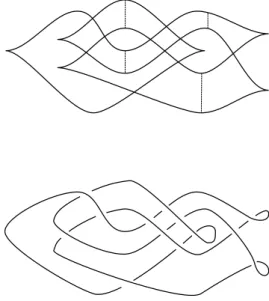
The front and Lagrangian projections of Λ in the previous theorem are shown on Figure 1 (note that this Legendrian knot also appears in the end of [18] as an example of Lagrangian slice knot).
Figure 1. Front and Lagrangian projections of a Legendrian representative of m(946).
This example confirms the analogy of this relation with a partial order. Whether or not it is a genuine partial order (meaning that Λ ≺ Λ′ and Λ′≺ Λ would imply
that Λ is Legendrian isotopic to Λ′) is neither proved nor disproved; the author
is unaware of any conjecture on how different the equivalence relation given by Λ ≺ Λ′
and Λ′
≺ Λ is from the Legendrian isotopy relation.
The knot Λ is the “smallest” Lagrangianly slice Legendrian knot (as it is clear from the Legendrian knot atlas of [6]); it is therefore the first natural candidate fo an example a non-reversible concordance. Using connected sums it is possible to construct more examples of this kind. Another class of examples in dimension 3 will appear in forthcoming work by J. Baldwin and S. Sivek in [1] where they construct concordances where the negative ends are stabilisations and the positive ones have non-vanishing Legendrian contact homology. In higher dimensions recent
results of Y. Eliashberg and E. Murphy [11] imply that if the negative end is loose (in the sense of [15]) then the Lagrangian concordance problem satisfies the h-principle. This can be used to prove further non reversible examples of Lagrangian concordances. Note that in both of those cases we still need pseudo-holomorphic curves techniques and the existence of maps in Legendrian contact homology to prove that the involved Lagrangian concordances cannot be reversed.
In order to prove the existence of the Lagrangian concordance claimed in The-orem 1.1 we use elementary Lagrangian cobordisms from [4] which we recall in Section 3. We also describe those elementary cobordisms in terms of Lagrangian projections as we will use those in Section 5 to compute maps between Legendrian contact homology algebras (LCH for short). As the negative end of the concor-dance is Λ0 which has non-vanishing LCH the actual argument not only relies on
the functoriality of Legendrian contact homology (as it is the case for the example of [11] and [1]) but also on a unknottedness result of Lagrangian concordances from Λ0to itself which follows from work of Y. Eliashberg and L. Polterovitch in
[12] which we state in the following:
Theorem 1.2. Consider the standard contact S3 (seen as the compactification
of the standard contact R3) and denote by K
0 the Legendrian unknot with −1
Thurston-Bennequin invariant (which corresponds to Λ0 in R3).
Let C be an oriented Lagrangian cobordism from K0 to itself. Then there is a
compactly supported symplectomorphism of R × S3 such that φ(C) = R × K 0.
Theorem 1.2 is proven in Section 6. Assuming then that a concordance C′
from Λ to Λ0 exists we could glue C to C′ to get a concordance from Λ0 to
Λ0 and applying Theorem 1.2 we deduce that the map induced in Legendrian
contact homology is the identity (as stated in Theorem 6.1). We conclude the proof of Theorem 1.1 in Section 7. In order to do so, we use the augmentation categories of Λ and Λ0 as defined in [2] and the functor between them induced by
the concordance to find a contradiction to the existence of a concordance from Λ to Λ0.
Remark 1.3. The main result was announced in the addendum in the introduction of [3]. When it was written bilinearised LCH was not known to the author. The original proof of the non-symmetry followed however similar lines. The idea is to construct several other concordances Ci from Λ0 to Λ (every dashed line in
Figure 1 is a chord where we can apply move number 4 of Figure 2 to get such a concordance). For each of those we computed the associated map similarly to what is done in Section 5. We then used Theorem 6.1 to prove that for each of them the composite map in Legendrian contact homology is the identity and deduce after some effort a contradiction. The existence of the augmentation category allows us to give a more direct final argument and use only one explicit concordance from Λ0 to Λ.
Acknowledgements. Most of this work was done while the author was supported first by a post-doctoral fellowship and after by a Mandat Charg´e de Recherche from the Fonds de la Recherche Scientifique (FRS-FNRS), Belgium. I
wish to thank both the FNRS and the mathematics department of the Universit´e Libre de Bruxelles for the wonderful work environment they provided. I also thank two anonymous referees whose comments and suggestions improved the exposition of the paper.
2. Lagrangian concordances and Legendrian contact
homology.
We recall in this section the main definition from [3].
Definition 2.1. Let Λ− : S1 ֒→ R3 and Λ+: S1 ֒→ R3 be two Legendrian knots
in R3. We say that Λ−is Lagrangian concordant to Λ+if there exists a Lagrangian
embedding C : R × Λ ֒→ R × R3such that
(1) C|(−∞,−T )×Λ= Id × Λ−.
(2) C|(T,∞)×Λ = Id × Λ+.
In this situation C is called a Lagrangian concordance from Λ−
to Λ+.
It was proven in [10] that two Legendrian isotopic Legendrian knots are indeed Lagrangian concordant. Another proof is given in [3] where we also proved that under Lagrangian concordances the classical invariants tb and r are preserved.
A Lagrangian concordance C is always an exact Lagrangian submanifold of R× R3in the sense of [9] and thus following [9] it defines a DGA-map
ϕC: A(Λ+) → A(Λ−)
where A(Λ±) denote the Chekanov algebras of the Legendrian submanifolds Λ±.
The homology of A(Λ) (denoted by LCH(Λ)) is called the Legendrian contact ho-mology of Λ (see [5] and [8]). This map is defined by a count of pseudo-holomorphic curves with boundary on C.
If C1 is a Lagrangian concordance from Λ0to Λ1 and C2 a Lagrangian
concor-dance from Λ1 to Λ2. We denote by C1#TC2 the Lagrangian concordance from
Λ0 to Λ2which is equal to a translation of C1 for t < −T and a translation of C2
for t > T . Then [9, Theorem 1.2] implies that there exists a sufficiently big T such that ϕC1#TC2 = ϕC1◦ ϕC2, in particular the association C → ϕC is functorial on
LCH.
3. Elementary Lagrangian cobordisms and their Lagrangian
projections.
For a Legendrian knot Λ in R3 we call the projection of Λ on the xz-plane along
the y direction the front projection of Λ. The projection on the xy plane along the zdirection is called the Lagrangian projection of Λ.
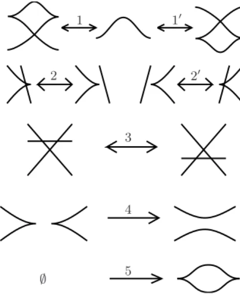
In order to produce an example of a non-trivial Lagrangian concordance we will use a sequence of elementary cobordisms as defined in [4] and [9]. A combination of results from [3], [4] and [9] implies that the local moves of Figure 2 can be realised by Lagrangian cobordisms (the arrows indicate the increasing R direction in R × R3). 1 1′ 2 2′ 3 4 5 ∅
Figure 2. Local bifurcations of fronts along elementary Lagrangian cobordisms.
The first three moves are Legendrian Reidemeister moves arising along generic Legendrian isotopies, in each case the associated cobordism is a concordance. The fourth move is a saddle cobordism which corresponds to a 1-handle attachment. The cobordism corresponding to the fifth move is a disk.
In Section 5 we will compute the induced map in Legendrian contact homol-ogy by a concordance. It will then be convenient to have a description of this concordance in terms of the Lagrangian projection. As it is easier in general to draw isotopy of front projections, we will use procedure of [16] to draw Lagrangian projections from front projections.
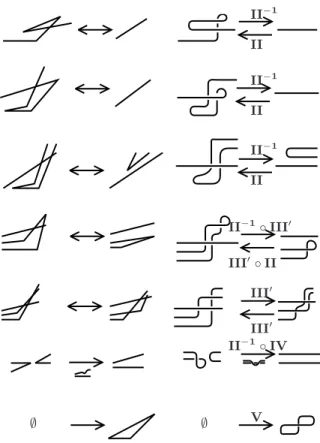
The idea is to write front projections in piecewise linear forms where the slope of a strand is always bigger than the one under it except before a crossing or a cusp. Such front diagrams are then easily translated into Lagrangian projections. In Figure 3 we provide, on the left, the elementary moves in front diagrams of this form associated to elementary cobordisms which we translate then, on the right, in terms of Lagrangian projections. As in Figure 2 the arrows represent the increasing time direction.
We label an arrow according to the corresponding bifurcation of the Lagrangian projection where II, III and III′
II−1 II II−1 II II−1 II II−1◦ III′ III′◦ II III′ III′ II−1◦ IV V ∅ ∅
Figure 3. Lagrangian projections of elementary cobordisms.
a cobordism from Λ−
to Λ+ induce a map from A(Λ+) to A(Λ−
) (i.e. following the decreasing time direction) we labelled a move in Figure 3 by the corresponding move from [14] following the arrow backward. As an example, if Λ−
differs from Λ+ by a move number II from [14] we will label the arrow by a II−1 as it is this
move we will use to compute the map from A(Λ+) to A(Λ−
). We denote by IV the saddle cobordism denoted Lsain [9] and by V the Lagrangian filling of Λ0denoted
by Lmi in [9]. In move number 4, we also provide an intermediate step which
corresponds to the creation of two Reeb chords one of which being then resolved by the cobordism (this procedure guaranties that the smallest newly created chord is contractible).
This language being understood we will be able to translate any bifurcation of fronts as a bifurcation of Lagrangian projections and we will keep drawing qualitative Lagrangian projections.
4. Example of a non-trivial concordance.
Using the moves of Figure 2 we are able to provide a non trivial Lagrangian con-cordance from Λ0to Λ. Note that the knot m(946) is the first Legendrian knot in
the Legendrian knot atlas of [6] with
gs(K) = 0 and max{tb(Λ)|Λ Legendrian representative of K} = −1,
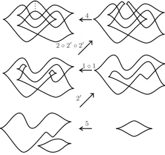
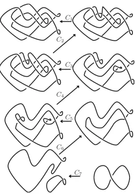
thus, following [3, Theorem 1.4], it is the simplest candidate for such an example. The bifurcations of the fronts along the non trivial concordance is given on Figure 4. 4 2 ◦ 2′◦ 2′ 1 ◦ 1 2′ 5
Figure 4. A non trivial Lagrangian concordance.
One can see that it is indeed a concordance either by using [3, Theorem 1.3] and deduce from tb(Λ) − tb(Λ0) = 0 that the genus of the cobordism is 0 or by
explictly seeing that the projection to R of C has only two critical points, one of index 1 and one of index 0 which implies that C is a cylinder.
5. Legendrian contact homology of Λ and some geometrical
maps.
We compute now the boundary operator on the Chekanov algebra of Λ (see [5]). As r(Λ) = 0 it is a differential Z-graded algebra over Z2freely generated by the double
points of the Lagrangian projection of Λ. The generators of A(Λ) are represented on Figure 5 where each ai has degree 1, each bi degree 0 and each ci degree −1.
a1 a2 a3 b6 a4 b5 b3 b4 c1 c2 a5 b1 b2
Figure 5. Generators of A(Λ).
The boundary operator on generators counts degree one immersed polygons with one positive corner and several negative corners and in our situation gives:
∂a1= 1 + a5c2b2+ b1b6+ b2 ∂a2= 1 + b2c2a4b2+ b2c2b3a5+ b6b4b2+ b6c1a5+ b6+ b2 ∂a3= 1 + a4b2c2+ b3a5c2+ b3+ b2b5 ∂a4= 1 + b3b1+ b2b4 ∂a5= b1b2 ∂b1= ∂b2= 0 ∂b3= b2c1 ∂b4= c1b1 ∂b5= b4b2c2+ c1a5c2+ c2+ c1 ∂b6= b2c2b2 ∂c1= ∂c2= 0.
It is then extended to the whole algebra by Leibniz’ rule: ∂(ab) = ∂(a)b+a∂(b). We will now compute the map between Chekanov algebras associated to the concordance C of Figure 4. At each step we use the results of [9] which give a combinatorial description of the map associated to each elementary cobordism.
On Figure 6 we see the bifurcations of the Lagrangian projections along C using the correspondence between front moves and Lagrangian moves of Figure 3, for convenience we split the first two steps in two steps each. For a cobordism Ciwe
denote the differential of the DGA associated to the upper level by ∂C+i and the one
corresponding to the lower level by ∂−
Ci (of course ∂ + Ci+1 = ∂
−
Ci). At each step we
compute the map associated to these moves between the corresponding Chekanov algebras heavily using the results of [9, Section 6]. We provide the precise section of this paper we use for each of the corresponding move. We decorate the labels of the bifurcations of the Lagrangian projections with subscripts precising the chords involved by each move.
C1 C2 C3 C4 C5 C6 C7
5.1. Map associated to C1.. The bifurcation associated to the cobordism C1
is IIab as in Figure 7. The computation of the map associated to this move is the
most involved of all the DGA maps described in [14] and [9].
b5 b4 a1 a2 b6 a3 a4 b3 c1 a5 c2 b1 b2 b5 b4 a1 a2 b6 a3 a4 b3 c1 a5 c2 b1 b2 a b Figure 7. IIab.
Following [9, Section 6.3.4], in order to compute ϕC1 we need first to know ∂ − C1. We have: ∂C1−a1= 1 + a5c2b+ b1b6+ b ∂C1−a2= 1 + b2c2a4b2+ b2c2b3a5+ b6b4b2+ b6c1a5+ b6c2a+ b6+ b2 ∂C1−a3= 1 + a4b2c2+ b3a5c2+ b3+ bb5+ ac2 ∂C1−a4= 1 + b3b1+ bb4 ∂C1−a5= b1b2 ∂C1−b1= ∂−C1b2= 0 ∂−C1b3= bc1 ∂−C1b4= c1b1 ∂−C1b5= b4b2c2+ c1a5c2+ c2+ c1 ∂−C1b6= b2c2b ∂C1−c1= ∂C1− c2= 0 ∂C1−a= b + b2 ∂C1−b= 0.
Which we compare to ∂+C1 computed above which gave ∂C1+a1= 1 + a5c2b2+ b1b6+ b2 ∂C1+a2= 1 + b2c2a4b2+ b2c2b3a5+ b6b4b2+ b6c1a5+ b6+ b2 ∂C1+a3= 1 + a4b2c2+ b3a5c2+ b3+ b2b5 ∂C1+a4= 1 + b3b1+ b2b4 ∂C1+a5= b1b2 ∂C1+b1= ∂+C1b2= 0 ∂+C1b3= b2c1 ∂+C1b4= c1b1 ∂+C1b5= b4b2c2+ c1a5c2+ c2+ c1 ∂+C1b6= b2c2b2 ∂C1+ c1= ∂+C1c2= 0.
A priori, in order to compute the associated map ϕC1 we need to order the
Reeb chord according to the length filtration (see [14, Section 3.1] and [9, Section 6.3.4]). This ensure that when computing ϕC1(a) we already know the image by
ϕC1 of any letter appearing in ∂ −
C1(a). But we actually do not need to understand
the whole filtration in a concrete example. For this note that for any generator d of A(Λ+) if b is not a letter appearing in ∂−
C1(d) then ϕC1(d) = d regardless of its
action. Thus in the end we need to understand the filtration on a1, a3, a4, b3and
b6. One easily see that the action of a1 can be made as big as we want without
changing any other action. Then from the fact that ∂±
decreases the action one get that h(a1) > h(a3) > h(a4) > h(b3) and that h(a1) > h(b6). This is enough to
proceed with inductive process (as b6 only appears in ∂(a1) we treat it as having
action greater than a3).
Also note that ∂C1−(a) = b = b + 0 which give v = 0 (following the notation
from [9]).
We start with b3 following the notation of [9, Section 6.3.4] we need to write
∂C1−b3=PB1bB2b . . . BkbAwhere all B′sare words with letters in the generator
of A(Λ+) (with lower action than b
3) and where every occurence of b in A follows
an occurence of a. In our situation we have ∂−
C1b3 = bc1= bA with A = c1 (and
we have no word of type Bi). Thus b3 is mapped to b3+ aA = b3+ ac1.
We then proceed for a4, we get ∂C1−a4 = 1 + b3b1+ bb4 = A1+ A2+ bA3 with
A1= 1, A2= b3b1 and A3 = b4(again no B’s). Only A3 is of interest here (as it
belongs to a monomial containing b) and implies that a4 is mapped to a4+ ab4.
For a3we have ∂ −
C1a3= 1 + a4b2c2+ b3a5c2+ b3+ bb5+ ac2. The only relevant
monomial is bb5implying that a3 is mapped to a3+ ab5.
As for b6 we have ∂−C1b6 = b2c2b = Bb. This implies that b6 is mapped to
Finally for a1 we have ∂C1−a1 = 1 + a5c2b+ b1b6+ b = A1+ A2b+ A3+ A4b
with the only relevant Ai being A2 = a5c2 and A4= 1 giving that a1 is mapped
to a1+ a5c2a+ a.
In summary we have that ϕC1 does the following:
a1→ a1+ a + a5c2a
a3→ a3+ ab5
a4→ a4+ ab4
b3→ b3+ ac1
b6→ b6+ b2c2a
and all other generators are mapped to themselves.
5.2. Map associated to C2.. The bifurcation associated to C2 is of type IVb
using the notations of Figure 8.
b5 b4 a1 a2 b6 a3 a4 b3 c1 a5 c2 b1 b2 a b b5 b4 a1 a2 b6 a3 a4 b3 c1 a5 c2 b1 b2 a
Figure 8. Saddle cobordism IVb.
An easy verification shows that the contractible Reeb chord b is simple (in the sense of [9]). We can thus apply [9, Proposition 6.17] and count immersed polygons with two positive corners (one on b). We get only three of those (the ± superscripts design postive and negative corners of the polygons):
a+2b−6b+a− b+4b+ b+5b+a−c−2.
Which gives that the map ϕC2 does the following:
a2→ a2+ b6a
b4→ b4+ 1
b5→ b5+ ac2
all other generators being mapped to themselves. This changes the differential as follows:
∂C2−a1= a5c2+ b1b6 ∂C2−a2= 1 + b2c2a4b2+ b2c2b3a5+ b6b4b2+ b6c1a5+ b2 ∂C2−a3= 1 + a4b2c2+ b3a5c2+ b3+ b5 ∂C2−a4= b3b1+ b4 ∂C2−a5= b1b2 ∂C2−b1= ∂ − C2b2= 0 ∂C2− b3= c1 ∂C2− b4= c1b1 ∂C2− b5= b4b2c2+ c1a5c2+ c1 ∂C2− b6= b2c2 ∂C2−c1= ∂C2−c2= 0 ∂C2−a= 1 + b2 ∂C2−b= 0.
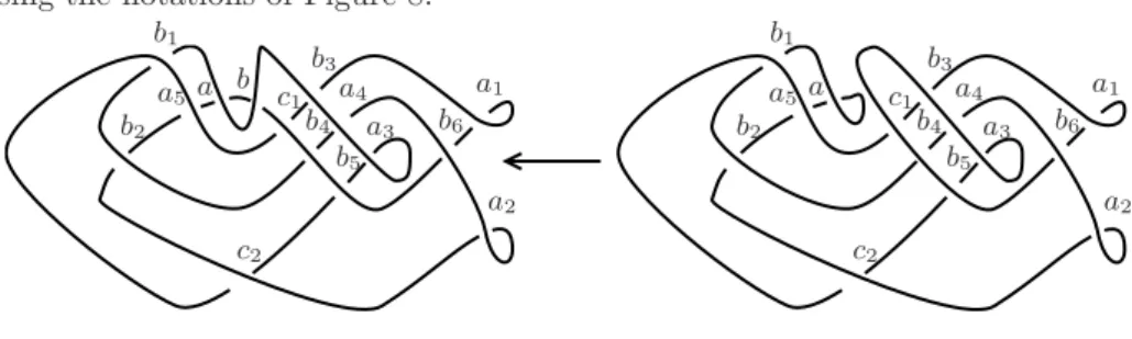
5.3. Map associated to C3.. Using the notation of Figure 9, the bifurcations
associated to C3 are given by first II−1b3c1 then II −1
a4b4 (going in the decreasing t
direction). b5 b4 a1 a2 b6 a3 a4 b3 c1 a5 c2 b1 b2 a a1 a2 b6 a5 c2 b1 b2 a b5 a3 Figure 9. II−1 b3c1◦ II −1 a4b4.
From ∂C3+(b3) = c1= c1+ v with v = 0 we deduce (following [9, Section 6.3.3])
that at the first bifurcation b3maps to 0 and c1maps to v thus to 0. This implies
maps to 0. Thus ϕC3 does the following:
b3→ 0
c1→ 0
a4→ 0
b4→ 0
all other generators being mapped to themselves.
5.4. Map associated to C4.. Following the notation of Figure 10, the
bifurca-tions associated to the cobordism C4are, again following the decreasing t direction,
first III′ b1a5athen II −1 a5b1. a3 b5 a1 a2 b6 a5 c2 b1 b2 a a1 a2 b6 c2 a b2 a3 b5 Figure 10. III′ b1a5a◦ II −1 a5b1.
To compute the map associated to III′
b1a5awe apply [9, Section 6.3.2] and get
that a5 maps to a5+ b1aand all other generators are mapped to themselves.
One computes that in the middle ∂(a5) = ∂C4+(a5) + ∂(b1a) = b1b2+ b1+ b1b2=
b1. Applying again [9, Section 6.3.3] we deduce that the bifurcation II−1a5b1 maps
a5and b1to 0. This implies that ϕC4 does the following:
a5→ 0
b1→ 0
a→ a
The differential at this step is: ∂C4−a1= 0 ∂C4−a2= 1 + b2 ∂C4−a= 1 + b2 ∂−C4b2= 0 ∂−C4b6= b2c2 ∂C4−a3= 1 + b5 ∂−C4b5= 0.
5.5. Map associated toC5.. Using the notation of Figure 11, the bifurcations
corresponding to C5are II−1a3b5 and II −1
ab2 (these are commutative).
a1 a2 b6 c2 a1 a2 a b2 a3 b5 b6 c2 Figure 11. II−1 a3b5◦ II −1 ab2.
One easily see that ϕC5 does the following:
a→ 0 b2→ 1
a3→ 0
b5→ 1
and all other generators are mapped to themselves. The differential becomes:
∂C5−a1= 0
∂C5−a2= 0
∂−C5b6= c2
∂C5− c2= 0.
a1 a2 b6 c2 a1 a2 Figure 12. II−1 b6c2.
We have that ϕC6 does:
a1→ a1
a2→ a2
b6→ 0
c2→ 0.
5.7. Map associated toC7and the compositionϕC.. The last part of C is
filling one of the components of the link on Figure 12 with a Lagrangian disk (lets say the one with Reeb chord a1). This has the effect of mapping the corresponding
chord to 0, thus ϕC7(a1) = 0 and ϕC7(a2) = a0where a0is the unique Reeb chords
of Λ0.
Combining this to the previous paragraphs we get that the map
ϕC= ϕC7◦ ϕC6◦ ϕC5◦ ϕC4◦ ϕC3◦ ϕC2◦ ϕC1
associated to the concordance of Figure 4 is:
a2→ a0
a1, a3, a4, a5, b1, b3, b6, c1, c2→ 0
b2, b4, b5→ 1.
6. Lagrangian concordances from Λ
0to itself.
The aim of this section is to prove the following:
Theorem 6.1. Let C be a Lagrangian concordance from Λ0 to Λ0 then the map
ϕc : A(Λ0) → A(Λ0) induced by C is the identity.
This follows from Theorem 1.2 of which we give a proof now.
Let C ⊂ R × S3 be an oriented Lagrangian cobordism from K
0to itself. First
note that since tb(K0) − tb(K0) = 0 it follows from [3] that C is topologically a
cylinder.
The symplectisation of S3 is symplectomorphic to C2\ 0 with its standard
symplectic form. Under this symplectomorphism the t-direction becomes the radial direction. A parametrisation of K0in S3is given by {(cos(θ), sin(θ))|θ ∈ [0, 2π)} ⊂
C2 i.e. Λ0 = R2∩ S3 ⊂ C2 where R2 = {(x, y)|x, y ∈ R} ⊂ C2. Thus C is a Lagrangian cylinder which coincides near 0 and outside a compact ball with the trivial Lagrangian plane, i.e. C1 = C ∪ {0} is local Lagrangian knot (following
the terminology of [12]). It follows from the main result of [12] that there exist a compactly supported Hamiltonian diffeomorphism φH such that φH(C1) = R2 ⊂
C2.
For ǫ > 0 we denote by Dǫthe ball of radius ǫ in C2. Take ǫ sufficiently small
so that Cǫ:= C1∩ Dǫ= R2∩ Dǫ. Since φH maps C1to R2then φH(Cǫ) ⊂ R2and
there exists a compactly supported diffeomorphism isotopic to the identity f of R2
such that f (φH(Cǫ)) = Cǫ. Using standard construction one can extend f to a
compactly supported Hamiltonian diffeomorphism ef of C2 (which by assumption
preserves R2). Thus φ
1 = ef ◦ φH is a compactly supported Hamiltonian
diffeo-morphism mapping C1 to R2 such that φ1|Cǫ = Id. Now standard application of
Moser’s path method leads to an Hamiltonian diffeomorphism φ′
supported in Dǫ
such that φ′ preserves R2 and φ′◦ φ
1|Dǫ′ = Id for ǫ′ << ǫ. Restricting φ′◦ φ1 to
C2\ {0} proves the theorem.
We are now able to prove Theorem 6.1.
Proof of Theorem 6.1. Take a contact embedding of (R3, ξ
0) → (S3, ξ0) as in [13,
Proposition 2.1.8] such that Λ0 is mapped to K0. This embedding induces a
symplectic embedding of R × R3 in R × S3≃ C2\ {0}. Under this identification
the concordance C maps to a concordance from K0to itself. Theorem 1.2 implies
that there exist a compactly supported symplectomorphism φ mapping C to the trivial cylinder of K0.
Since φ is the identity near ±∞, for any cylindrical almost complex structure J on R × S3admissible (in the sense of [7]) for the trivial concordance we get that
(φ−1)∗
J is admissible for the original concordance C. This implies the induced map by C is the same map as the one induced by R × K0 which is the identity
(because the only degree 0 pseudo-holomorphic curve on the trivial concordance is the trivial one). Since H(A(Λ0)) = A(Λ0) and the induced map in homology by
ϕC do not depends on auxiliary choices, we get that the map do not depend on
the choice of the almost complex structure cylindrical at infinities. This conclude the proof.
7. Non symmetry of Lagrangian concordances.
In order to prove Theorem 1.1 we use the augmentation category of Λ denoted by
Aug(Λ). This is an A∞-category defined in [2] whose objects are augmentations of
the Chekanov algebra and morphisms in the homological category are bilinearised Legendrian contact cohomology groups.
Recall that an augmentation ε of a DGA (A, ∂) over Z2 is simply a DGA map
from (A, ∂) to (Z2,0).
Bilinearised cohomology groups are generalisations of linearised Legendrian contact cohomology groups (as defined in [5]) introduced in [2] using two aug-mentations instead of one and keeping track of the non-commutativity of A(Λ). Basically for two augmentations ε1and ε2and a word b1. . . bkin ∂a the expression
X
j
ε1(b1)ε1(b2) . . . ε1(bj−1) · bj· ε2(bj+1) . . . ε2(bk)
contributes to dε1,ε2a.
Dualising dε1,ε2 leads to bilinearised Legendrian contact cohomology differential
µ1ε1,ε2 : Cε1,ε2(Λ) → Cε1,ε2(Λ) (where Cε1,ε2(Λ) is the vector space generated by
Reeb chords of Λ) whose homology forms morphisms space in the homological category of the augmentation category. Higher order compositions are defined using similar considerations with more than 2 augmentations. For instance the composition of morphisms µ2
ε1,ε2,ε3 is defined as the dual of the map d ε3,ε2,ε1 2 which
to a word b1. . . bk in ∂a associates
X
i,j
ε3(b1) . . . ε3(bi−1) · bi· ε2(bi+1) . . . ε2(bj−1) · bj· ε1(bj+1) . . . ε1(bk).
We are now ready to prove Theorem 1.1.
Proof of Theorem 1.1. The first part on the existence of the concordance has been
proved in Section 4. It remains to prove that no concordance from Λ to Λ0 exists.
Assume that such a concordance C′
exists and denote by ϕC′ : A(Λ0) → A(Λ)
the induced map. Let C be the concordance of Section 5 which induced the map ϕC.
The concatenation of C′
with C leads to a concordance from Λ0 to itself.
Theorem 6.1 implies that the map induced by this concatenation is Id : A(Λ0) →
A(Λ0). Hence by [9, Theorem 1.2] we get that ϕC◦ ϕC′ = Id.
Now following [2, Section 2.4] we get that ϕC′ induces an A∞-functor FC′ :
Aug(Λ) → Aug(Λ0) (obtained by dualising the components of the map ϕC′).
Sim-ilarly ϕC induces an A∞-functor FC : Aug(Λ0) → Aug(Λ). From ϕC◦ ϕC′ = Id
we get that FC′◦ FC= Id.
Note that A(Λ0) has only one augmentation ε0 (which maps a0 to 0). By
definition of FC its action on the object of the augmentation category is given
ϕC ◦ ε0 = ε1 where ε1 is the first augmentation of Table 1. Table 1 also shows
another augmentation of A(Λ) we will use to compute bilinearised cohomology groups.
b1 b2 b3 b4 b5 b6
ε1 0 1 0 1 1 0
ε2 1 0 1 0 0 1
Table 1. Two augmentations of A(Λ).
We will now show that the two augmentation ε1and ε2 are not equivalent.
Table 2 gives the bilinearised differential for all possible pairs out of those two augmentations (as b1and b2are always mapped to 0 we omit them from the table).
a1 a2 a3 a4 a5 b3 b4 b5 b6 dε1,ε1 b 2 b2 b3+ b2+ b5 b2+ b4 b1 c1 0 c1 c2 dε2,ε2 b 1+ b2+ b6 b2+ b6 b3 b3+ b1 b2 0 c1 c2+ c1 0 dε1,ε2 b 1+ b2 b6+ b2 b3+ b5 b3+ b4 0 c1 c1 c1 0 dε2,ε1 b 6+ b2 b6+ b4 b3+ b2 b1+ b2 b1+ b2 0 0 c2+ c1 0
Table 2. Bilinearised differentials for Λ.
Notice that for linearised LCH (the first two lines) there are no non-trivial homology in degree −1 whereas for the mixed augmentation there is always a generator of degree −1. It follows then from [2, Theorem 1.4] that the two aug-mentations ε1and ε2 are not equivalent.
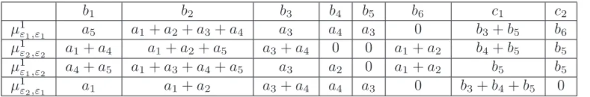
In order to conclude, one must study the compositions in the augmentation category and its homological category, thus we need to consider the bilinearised cohomology groups. From Table 2 we get that the bilinearised differentials in cohomology are those given in Table 3.
b1 b2 b3 b4 b5 b6 c1 c2 µ1ε1,ε1 a5 a1+ a2+ a3+ a4 a3 a4 a3 0 b3+ b5 b6 µ1 ε2,ε2 a1+ a4 a1+ a2+ a5 a3+ a4 0 0 a1+ a2 b4+ b5 b5 µ1 ε1,ε2 a4+ a5 a1+ a3+ a4+ a5 a3 a2 0 a1+ a2 b5 b5 µ1 ε2,ε1 a1 a1+ a2 a3+ a4 a4 a3 0 b3+ b4+ b5 0 Table 3. µ1 εi,εj on Λ.
From Table 3 we can see that LCH1
ε1 has one generator [a1] = [a2] (since
a1+a2= µ1ε1(b2+b3+b4)) and that LCHε10 has dimension 0 (since b6= µ1ε1(c2)). As
FC′◦FCis the identity we get that H(FC1′)◦H(FC1) : LCHε0(Λ0) → LCHε0(Λ0) is
the identity. This implies that in the homological category H(F1
LCHε0(Λ0) is surjective in particular the only generator [a2] of LCHε11(Λ) is
mapped to [a0] the generator LCHε01(Λ0).
In order to understand the compositions in the category, we need to compute ∂2ε1,ε2,ε1 which gives a1→ b1b6 a2→ c2a4+ c2a5+ b6b4 (1) a3→ b2b5 a4→ b3b1+ b2b4 a5→ b1b2 b3→ b2c1 b4→ c1b1 b6→ c2b2+ b2c2.
From Formula (1) we see that µ2
ε1,ε2,ε1(a5, c2) = a2 ∈ Cε1,ε1(Λ). As the
com-position [x] ◦ [y] in the homological category is given by [µ2(x, y)] we get that
[a5] ◦ [c2] = [a2]. Since FC′ is an A∞-functor we get that H(FC′1) preserves this
composition (see [2, Section 2.3]) thus we have that 0 6= [a0] = H(FC1′)([a2]) =
H(F1
C′)([a5]) ◦ H(FC1′)([c2]). However H(FC1′)([c2]) ∈ LCHε0−1(Λ0) ≃ {0}. Thus
[a0] = H(FC1′)([a5]) ◦ 0 = 0, this contradicts the existence of FC′ and hence the
existence of C′
. Thus Λ 6≺ Λ0.
References
[1] J. Baldwin and S. Sivek, Contact invariants in sutured monopole and instanton homology,in preparation. —-.
[2] F. Bourgeois and B. Chantraine, Bilinearised Legendrian contact homology and the augmentation category. ArXiv e-prints, to appear in ”Journal of Symplectic Geom-etry” (2012). 1210.7367
[3] B. Chantraine, Lagrangian concordance of Legendrian knots. Algebr. Geom. Topol. 10 (2010), 63–85. MR 2580429 (2011f:57049)
[4] B. Chantraine, Some non-collarable slices of Lagrangian surfaces. Bull. Lond. Math. Soc. 44 (2012), 981–987.
[5] Y. Chekanov, Differential algebra of Legendrian links. Invent. Math. 150 (2002), 441–483. MR MR1946550 (2003m:53153)
[6] W. Chongchitmate and L. Ng, An atlas of Legendrian knots. Exp. Math. 22 (2013), 26–37. MR 3038780
[7] T. Ekholm, Rational symplectic field theory over Z2 for exact Lagrangian
[8] T. Ekholm, J. Etnyre, and M. Sullivan, The contact homology of Legendrian sub-manifolds in R2n+1. J. Differential Geom. 71 (2005), 177–305. MR MR2197142
[9] T. Ekholm, K. Honda, and T. K´alm´an, Legendrian knots and exact Lagrangian cobordisms. ArXiv e-prints (2012). 1212.1519
[10] Y. Eliashberg and M. Gromov, Lagrangian intersection theory: finite-dimensional approach. In Geometry of differential equations, Amer. Math. Soc. Transl. Ser. 2 186, Amer. Math. Soc., Providence, RI 1998, 27–118. MR 1732407 (2002a:53102) [11] Y. Eliashberg and E. Murphy, Lagrangian caps. Geometric and Functional Analysis
(2013), 1–32.
[12] Y. Eliashberg and L. Polterovich, Local Lagrangian 2-knots are trivial. Ann. of Math. (2) 144 (1996), 61–76. MR MR1405943 (97g:58055)
[13] H. Geiges, An introduction to contact topology. Cambridge Studies in Advanced Mathematics 109, Cambridge University Press, Cambridge 2008. MR 2397738 (2008m:57064)
[14] T. K´alm´an, Contact homology and one parameter families of Legendrian knots. Geom. Topol. 9 (2005), 2013–2078 (electronic). MR MR2209366
[15] E. Murphy, Loose Legendrian Embeddings in High Dimensional Contact Manifolds. ArXiv e-prints (2012). 1201.2245
[16] L. Ng, Computable Legendrian invariants. Topology 42 (2003), 55–82. MR 1928645 (2003h:57038)
[17] D. Rolfsen, Knots and links. Mathematics Lecture Series 7, Publish or Perish Inc., Houston, TX 1990. Corrected reprint of the 1976 original. MR MR1277811 (95c:57018)
[18] S. Sivek, Monopole Floer homology and Legendrian knots. Geom. Topol. 16 (2012), 751–779. MR 2928982
Baptiste Chantraine, Laboratoire de Math´ematiques Jean Leray, Universit´e de Nantes, 2 rue de la Houssini`ere, BP 92208 , F-44322 Nantes Cedex 3, France. E-mail: [email protected]