Diapycnal Advection by Double Diffusion and Turbulence
in the Ocean
by
Louis Christopher St. Laurent
B.S. University of Rhode Island, 1994Submitted in partial fulfillment of the requirements for the degree of Doctor of Philosophy
at the
MASSACHUSETTS INSTITUTE OF TECHNOLOGY and the
WOODS HOLE OCEANOGRAPHIC INSTITUTION September 1999
@1999
Louis C. St. Laurent. All rights reserved.The author hereby grants to MIT and to WHOI permission to reproduce and to distribute copies of this thesis document in whole or in part.
Signature of Author ... ...
Joint Program in Physical Oceanography Massachusetts Institute of Technology Woods Hole Oceanographic Institute Augyst 4, 1999
Certified by ... ...
. ...
Raymond W. Schmitt Senior Scientist Woods Hole Oceanographic Institute
Thesis Supervisor Accepted by ...
W. Brechner Owens Chairman, Joint Committee for Physical Oceanography Massachusetts Institute of Technology Woods Hole Oceanographic Institute
Diapycnal Advection by Double Diffusion and Turbulence in the Ocean
by
Louis C. St. Laurent
Submitted in partial fulfillment of the requirements for the degree of Doctor of Philosophy at the Massachusetts Institute of Technology and the Woods Hole
Oceanographic Institution in August 1999 Abstract
Observations of diapycnal mixing rates are examined and related to diapycnal advection for both double-diffusive and turbulent regimes.
The role of double-diffusive mixing at the site of the North Atlantic Tracer Release Experiment is considered. The strength of salt-finger mixing is analyzed in terms of the stability parameters for shear and double-diffusive convection, and a nondi-mensional ratio of the thermal and energy dissipation rates. While the model for turbulence describes most dissipation occurring in high shear, dissipation in low shear is better described by the salt-finger model, and a method for estimating the salt-finger enhancement of the diapycnal haline diffusivity over the thermal diffusivity is proposed. Best agreement between tracer-inferred mixing rates and microstructure based estimates is achieved when the salt-finger enhancement of haline flux is taken into account.
The role of turbulence occurring above rough bathymetry in the abyssal Brazil Basin is also considered. The mixing levels along sloping bathymetry exceed the levels observed on ridge crests and canyon floors. Additionally, mixing levels modulate in phase with the spring-neap tidal cycle. A model of the dissipation rate is derived and used to specify the turbulent mixing rate and constrain the diapycnal advection in an inverse model for the steady circulation. The inverse model solution reveals the presence of a secondary circulation with zonal character. These results suggest that mixing in abyssal canyons plays an important role in the mass budget of Antarctic Bottom Water.
Thesis Supervisor: Raymond W. Schmitt
Acknowledgments
In my final year as an undergraduate at the University of Rhode Island, I spoke with an adjunct faculty member of the physics department about my interests in physical oceanography. Lou Goodman immediately mentioned the MIT/WHOI program. In particular, he wrote the names of several faculty members on a piece of paper, adding, "I respect these people not only as scientists, but also as friends." A day later, I found brief descriptions of research interests for each of the names Lou provided, and I decided to make some calls. Ray Schmitt was first name on the list. His research sounded interesting, and besides, he was very friendly on the phone. I didn't see any need to call the remaining people.
My initial judgment was appropriate. Ray's enthusiasm is contagious, and he introduced me to numerous exciting problems in oceanography. The work I began with Ray my first summer became the seed for my thesis work. His guidance allowed me to make steady progress on interesting problems while I was still learning the ropes. I am fortunate to have found such a competent mentor.
As a member of a research team, my thesis work would not have progressed without the additional guidance of others. The scope of John Toole's expertise is rivaled by few in physical oceanography. He has tackled problems ranging from the mass budget of the Indian Ocean (a spatial scale of millions of meters) to the molecular dissipation of scalar variance (a spatial scale of millimeters). I have exploited many of John's insights in my work. Kurt Polzin too has been a great asset. The quality of the microstructure data on which my work relied was assured by Kurt's efforts. Francesco Paparella joined the team just in time to allow me to run memory-greedy calculations on his workstation. Finally, the group's technical support, in particular Ellyn Montgomery and Gwyneth Packard, maintained the
resources I used everyday.
My experience in graduate school was overwhelmingly positive, largely because of the people I met. My close classmates, Brian Arbic, Albert Fischer, Stephanie Harrington and Steve Jayne deserve special mention. Tom Marchitto, Mike Braun and Patricia Kassis also became close friends.
There are only a few people who know the whole story, which is probably for the best. My friends often hear me joke about how I was not a member of the
"gifted class." The joke would not be lost on Jack Crowley. Most of all, I have shared so much of my story with a geologist I met at URI. When family friends learn that my research doesn't involve dolphins, it is Jenn who saves the moment for science, with stories of her volcano adventures. There are many other things that Jenn does so well, and it is to her that I am the most grateful.
This work was supported by contracts N00014-92-1323 and N00014-97-10087 of the Office of Naval Research and grant OCE94-15589 of the National Science Foundation.
Contents
1 Introduction
1.1 Thermodynamic Considerations . . . . 1.2 Dynamical Considerations . . . . 2 The Contribution of Salt Fingers to Vertical Mixing in the North
Atlantic Tracer Release Experiment
2.1 Introduction . . . . 2.2 Qualitative Evidence for Salt Fingers at the NATRE Site 2.3 Quantitative Assessment of Salt-Finger Mixing . . . . . 2.3.1 Description of Data . . . . 2.3.2 The Dissipation Ratio Model . . . . 2.3.3 Method of Analysis . . . . 2.3.4 Statistical Treatment of Dissipation Data . . . .
2.3.5 R esults . . . . 2.4 Mixing at the NATRE Site . . . . 2.4.1 Vertical Mixing Influenced by Salt Fingers . . . . 2.4.2 Estimates of Diapycnal Advection . . . . 2.5 D iscussion . . . . 3 Buoyancy Forcing Above Rough Bathymetry in the Aby
Basin
3.1 Introduction . . . . 3.2 D issipation . . . .
3.2.1 Description of Dissipation Data . . . .
. . . . . 19 . . . . 22 . . . . . 24 . . . . . 24 . . . . . 28 . . . . . 31 . . . . . 35 . . . . . 38 . . . . . 46 . . . . . 46 . . . . . 51 . . . . . 56 ssal Brazil 63 . . . . . 63 . . . . . 67 . . . . . 67 . . .
Spatial Bias . . . . 73
Temporal Bias . . . . 73
3.2.2 Mechanisms of Bottom Generation . . . . 76
3.2.3 A Model for the Dissipation . . . . 79
3.3 The Inverse Model . . . . 80
3.3.1 Model Equations . . . . 80
3.3.2 Treatment of Data . . . . 82
3.3.3 Linear Algebraic Equations . . . . 88
3.3.4 Results . . . . 89
Shallow Flow . . . . 92
Deep Flow . . . . 96
Model Sensitivity . . . . 103
Deep Upwelling . . . . 104
3.4 Mixing Rates and Flow in an Abyssal Canyon . . . . 106
3.5 Discussion . . . . 113
4 Conclusions 121 4.1 Salt-Finger Mixing . . . . 123
4.2 Abyssal Dissipation . . . . 125
Chapter 1
Introduction
The ocean is stratified by heat and salt. At the ocean's surface, these properties are controlled by the sun, wind and rain. If the ocean were stagnant, temperature and salinity conditions at the sea surface would not mix into the oceanic interior. The molecular diffusion of seawater would support a thin boundary layer between surface and abyssal properties. In truth, much of the ocean's depth is
strati-fied. The gradients of heat, salt and density are strongly aligned in the vertical. Thus, the vertical, or diapycnal direction, is the direction of consequence for the production of buoyancy forces by mixing.
Questions regarding the role of vertical mixing in driving the ocean's circula-tion have persisted for many years. Some of the first dynamical ideas for both the abyssal (Stommel 1957, 1958) and the thermocline (Robinson and Stommel 1959) circulations relied heavily on the notion that a vertical diffusion of heat acts to balance the vertical advection occurring throughout the ocean's interior. Such a balance was invoked by Munk (1966), who examined vertical property distributions in the abyssal Pacific. Munk's calculations implied that a turbulent diffusivity of k ~ 0(1 cm2 s1) is needed to balance an 0(10 Sv) global deep-water
production through uniform upwelling, and this mixing-rate estimate became the benchmark for all assessments of oceanic mixing.
Direct observations of temperature structures at vertical scales of O(1 cm) provide a means of estimating the rate of molecular dissipation, and these "mi-crostructure" derived estimates of oceanic mixing-rates were introduced by Os-born and Cox (1972). Early microstructure observations from the Pacific (Gregg
1980) and Atlantic (Gregg and Sanford 1980), the later including Gulf Stream and Bermuda Slope data, indicated that mixing levels in thermocline were an order of magnitude weaker than Munk's estimate. Additional microstructure observations have demonstrated that weak 0(0.1 cm2 s-1) mixing rates extend into the abyssal interior (Moum and Osborn 1986; Toole et al., 1994). While larger mixing rates have been observed in high-shear regions such as the Equatorial Undercurrents (Osborn 1980; Gregg et al., 1985) and the surface Ekman-layer (Oakey 1985), the vastness of the oceanic interior limits the global influence of these special regions. The vertical mixing measured by microstructure is an intrinsically small-scale phenomenon, and its mechanics are not obviously related to larger-scale conse-quences. For this reason, the influence of vertical mixing on the ocean's circulation is not easily established. Ocean general circulation models (OGCMs) parameter-ize vertical mixing as a bulk eddy-diffusivity, often specified as a global constant. While these models are prone to producing spurious diapycnal mixing by laterally mixing across sloping isopycnals (Veronis 1975), their ability to resolve the global and decadal (centennial) scales of the wind driven and thermohaline circulations make OGCMs valuable for assessing the role of vertical mixing. In particular, Bryan (1987) assessed the implications of vertical mixing on meridional overturn-ing and poleward heat-transport usoverturn-ing both thermocline theory and an OGCM. Bryan used a closed-sector geometry and found that a realistic thermohaline-circulation results when O(1 cm2 s-1) diffusivities are specified. Such OGCMs
with closed-sector basins have been modified to incorporate more sophisticated parameterizations of buoyancy forcing. Marotzke (1997) specified large diffusivi-ties in thin boundary-layers around the basin, while Zhang et al. (1999) consider both "relaxation" and "mixed" boundary conditions for temperature and salinity. Both studies find that the overturning strength of the thermohaline cell is de-pendent on k2/3. However, other OGCM studies using a global basin (Cox 1989;
Toggweiler and Samuels 1995) find the structure and strength of the thermohaline flow is strongly influenced by the Antarctic Circumpolar Current (ACC). Togg-weiler and Samuels (1998) find that the ACC drives a wind-powered thermohaline circulation without vertical mixing in the interior, consistent with predictions of scaling relations (Gnanadesikan 1999).
diffusivity and the thermohaline circulation, the parameterizations of mixing in such models are poor. The influence of geographic and depth dependence of diapycnal mixing on circulation dynamics have not been thoroughly researched. Furthermore, the relationships between large-scale hydrography and buoyancy forcing remain vague. Observational programs that relate the mechanics of small-scale mixing with larger small-scales of motion remain necessary.
This thesis will address the implications of data collected during two such observational programs. The first case considered (chapter 2) involves double-diffusive mixing in the North Atlantic subtropical thermocline. The second case (chapter 3) considers turbulent mixing in the abyssal Brazil Basin. Both of these problems are attractive because they address poorly understood mixing-regimes. In both cases, the work will begin at the small scale with microstructure-derived mixing rates. The mixing rates will be used to derive the buoyancy fluxes that act between density layers of stratified flow. Diapycnal advection, the component of flow perpendicular to surfaces of potential density, will be of primary interest. Though a dynamically important quantity, diapycnal advection is a poorly con-strained quantity in nearly all contexts of physical oceanography. It appears in the advective budgets for heat and salt, and also in the vorticity budget, where the divergence of diapycnal velocity acts as a vortex stretching mechanism. In this way diapycnal advection fundamentally links the small-scale processes of mixing to the larger-scale patterns of circulation.
In chapter 2, the case of mixing in the North Atlantic thermocline will be exam-ined. This study is the consequence of a field program begun in 1992, The North Atlantic Tracer Release Experiment (NATRE). The experiment was conducted to document the details of mixing in the pycnocline and consisted of both a mi-crostructure profiling and a tracer-release phase. The tracer work was conducted by Jim Ledwell and his colleagues, and is described by Ledwell et al. (1993, 1998). The results derived from the 2.5 year tracer evolution have greatly benefited the study of mixing in the ocean.
Prior to the tracer release result, the thermocline mixing-rates inferred from microstructure observations were questioned. The diffusivity estimates consis-tently indicated k < 0.1 cm2 s-I, a value only 100 times larger than the molecular
of magnitude less than the diffusivity deduced by Munk (1966) for the abyssal ocean. Issues related to undersampling and intermittency of mixing were cited as reasons for microstructure estimates being low (Gibson, 1982). Additionally, the framework for estimating diffusivity from microstructure, first proposed by Os-born and Cox (1972), has been called into question (Davis 1994). However, after 30 months of evolution, the tracer cloud described by Ledwell et al. (1998) cov-ered 0(1000 km)2 of the North Atlantic subtropical gyre, and the tracer result of
k - 0.1 cm2 s-I showed little dependence on space or time. The tracer result has produced confidence in the 0(0.1 cm2s-1) thermocline mixing-rates consistently
estimated from microstructure.
In that the internal-wave climate of the thermocline is known to conform to the canonical description of the Garret and Munk spectrum (GM; Garrett and Munk 1975; Munk 1981), mixing in the thermocline has been interpreted in terms of wave instabilities and nonlinear interactions of the GM spectrum (Henyey et al. 1986; Polzin et al., 1995). However, the mechanism of double diffusion has long been identified as a possible additional contributor to mixing in the thermocline (Stern 1960). In particular, the so-called "salt finger" form of double diffusion is favored at mid-latitudes, where excess evaporation over precipitation causes the salinity to decrease with depth. The potential energy stored in the top-heavy salinity profile provides the energy source for mixing. Though the instability conditions of salt fingers have been understood for some time, an assessment of salt-finger mixing in the thermocline has been elusive. Since internal waves are an ubiquitous feature of the thermocline, most past work has assumed that all mixing in the pycnocline can be attributed to wave-field instabilities, even when the halocline favors the salt-finger instability.
The work presented in chapter 2 will generalize a thermodynamic model for velocity and shear microstructure which permits the signal of salt-finger mix-ing to be discerned in conditions where shear and internal waves are also active mixing mechanisms. While shear-produced turbulence acts to produce a down-gradient density-flux, fingers flux density updown-gradient. The two processes compete to determine the direction of the density flux and the direction of the diapycnal advection. The data presented in chapter 2 show that for the shallow depths of the pycnocline (z < 400 m) at the NATRE site, the divergence of the haline
com-ponent of the buoyancy flux dominates over the thermal contribution, owing to the salt-finger enhancement of the salinity flux. This leads to a downward diapy-cnal advection that is not possible by turbulent mixing alone. Thus, salt-finger mixing represents a distinct mechanism of water-mass conversion. The results of chapter 2 provide observational evidence for the role of salt-fingers in modifying upper ocean temperature-salinity structure.
In chapter 3, the case of mixing in the abyssal Brazil Basin will be examined. Like the NATRE study, microstructure measurements were made to compliment a tracer-release experiment, the Brazil Basin Tracer Release Experiment (BBTRE, Polzin et al., 1997; Ledwell et al., 1999). This experiment was undertaken to doc-ument the rates and mechanisms of mixing in the abyssal ocean. The BBTRE mi-crostructure and tracer observations constitute the most extensive abyssal-mixing data set ever collected. However, previous estimates of deep mixing-rates have been made. In particular, Hogg et al. (1982) deduced that a vertical diffusivity of k ~ (2 - 4) cm2s 1 is needed to close the heat and mass budget of the Brazil
Basin's densest water class. This estimate, and those for other abyssal basins, suggested that mixing rates in the deep could be orders of magnitude larger than in the thermocline.
The dense water of the abyss is far removed from contact with the atmosphere, where wind stress acts to input vorticity and drive circulation. Instead, the ocean's densest waters are formed in remote high-latitude seas and then advected to mid latitudes by boundary currents. In the abyssal interior, flow is supported by buoyancy forcing. These ideas were first proposed by Stommel (1957). Lacking specific details about how buoyancy forcing is distributed, Stommel and Arons (1960) examined a model where upwelling occurs uniformly throughout the abyss. While boundary currents are still recognized as a fundamental component of the deep circulation, ideas about buoyancy forcing have changed.
An association between enhanced mixing-rates and rough topography has been noted in prior reports (Polzin et al., 1997; Toole et al., 1997). These data suggest that mixing is related to internal-wave processes occurring well into the stratified water above the bathymetry. Bathymetric charts show systems of seamounts and other rough bathymetric features implying that enhanced buoyancy-forcing near abyssal topography will lead to complex and varied flow structures.
The work presented in chapter 3 will assimilate observations of enhanced mix-ing near the Mid Atlantic Ridge with an inverse model describmix-ing the large-scale flow. This model constrains the diapycnal advection to conform in a self consis-tent way with both the thermodynamics dictated by the microstructure, and the vorticity, heat and mass budgets dictated by the hydrography. Steady geostrophic dynamics are assumed valid, and the contribution of vortex stretching by diabatic and adiabatic flow will be assessed.
Concluding remarks will be made in chapter 4. There, the value of the findings from the two mixing regimes I examined will be discussed. This discussion will address implications for the work that extend beyond the specific regional nature of the two problems presented. In the remaining sections of this introductory chapter, some thermodynamical and dynamical considerations will be discussed.
1.1
Thermodynamic Considerations
At the largest scales, variance is input into the ocean through atmospheric forcing. The global budgets of two important variance quantities have been formulated; thermal variance (Joyce 1980) and mechanical energy (Lueck and Reid 1984). Both of these studies formulated the input of variance at large scales by air/sea interaction, and the removal of variance at small scales by mixing. At the smallest scales, variance is dissipated by the molecular diffusion of seawater. Thus, rates of variance dissipation are synonymous with the rates of small-scale mixing.
The thermodynamic equations for thermal variance and turbulent kinetic en-ergy (TKE) are central to the mixing-rate estimation problem. These equations are derived from Reynolds decomposition of the Navier-Stokes and heat equations, as discussed by Monin and Yaglom (1971) and Tennekes and Lumley (1972). In standard tensor notation of the variables of fluid mechanics, the budget for ther-mal variance is
a-
-02 +a
/-
U 2 +u,0 2 -Do
W2at
axi
axi
Average quantities in (1.1) are denoted by upper case (UJ , 0), and fluctuating
quantities by lower case (ui, 0). The terms that precede the equal sign represent the physical rearrangement of thermal variance in time and space. The three terms in parenthesis denote advection of thermal variance by the mean flow (Uj) and the fluctuating flow (uj), and by molecular diffusion Do. The source and sink terms follow the equal sign, with the rate of thermal variance extraction from the mean temperature field given by 2uj0(88/8xj), while the rate of dissipation by molecular diffusion Do is given by
x
= 2Do(80/8xa) 2. The budget for TKE is inmany ways analogous,
+
1 8~ 1- 1i 8
-at 2 &xi U2 q2 2 ziuau v_ xi 2
-Uiu axi - E - -wp, (1.2)
where (1/2)q2 = (1/2)(U2 + v2 + w2) is the TKE per unit mass and c
-(1/2)v(auj/8xj - aul/axa) 2 s the dissipation rate. The spatial rearrangement
terms in parenthesis denote advection of TKE by the mean flow (Uj) and the fluctuating flow (uj), as well as the energy transfer by pressure work and viscous diffusion. The first of the source/sink terms in (1.2), -uiuj(Uj/80xj), represents the exchange of energy between the mean flow and the turbulence. For the class of turbulence of concern here, the smallest scales of the flow are damped by vis-cosity, and the cascade of energy is from the larger scales of the mean flow such that -iuu( 9Uj/8xj) > 0, so that this term is referred to as the production of TKE. This is in contrast to so-called "geostrophic turbulence", where the direc-tion of the energy transfer can be from small scales to large, as discussed by Starr (1968). Of the remaining terms, the viscous dissipation E represents the loss of TKE to molecular viscosity. The final term represents the exchange of TKE with potential energy by buoyancy flux. In stably stratified conditions, the exchange is from kinetic energy to potential energy, so the buoyancy flux term acts as a sink. Within the context of oceanic turbulence, the averaging associated with the Reynolds decomposition is applied over an ensemble of many observations. This procedure produces an energy balance that is both spatially and temporally av-eraged, and the following assumptions are applied: (1) the diffusive transport of
thermal variance Doa(92
)/axi
and the viscous transport of energy v(q2/2)/8x are ignored as they scale as small compared to the production terms, (2) the triple correlation and pressure work advection terms are assumed to be spatially homogeneous and thus vanish when differentiated, as indicated by experimental work (Rohr et al., 1988; Itsweire et al., 1993), (3) the mean flow parameters are functions of the vertical coordinate only, and (4) over the scales of the temporal and spatial averaging, the distributions of thermal variance and TKE are sta-tionary in time and homogeneous in space, so that the advective rates of change(a/t + Uia/axi) vanish. These assumptions lead to greatly simplified variance
budgets. A simplified budget for thermal variance was proposed by Osborn and Cox (1972),
2(wO) E2 + X= 0.
(1.3)
In this expression, the production of thermal variance by vertical flux is directly balanced by dissipation. Modeling the flux as a Fickian diffusion, the Osborn-Cox
expression implies the thermal eddy-diffusivity relation ko = (1/2)XE2 2
.
Thereduction of the (1.1) to (1.3) requires validity of numerous assumptions, all of which are difficult to justify for geophysical flows (Davis 1994). However, the production-dissipation balance stated in (1.3) can be derived from considerations independent of the thermal variance budget. This derivation is given by Winters and D'Asaro (1996), who show that the justified application of (1.3) relies on the definition of the mean temperature gradient
E2.
These authors proposeE2
should be defined from a reference stratification exhibiting the minimum potential energy when compared to all possible rearrangements of a given profile of temperature. In practice, the "Thorpe sorting" technique (Dillon, 1984; after Thorpe 1977) commonly employed in microstructure analyses achieves the desired result.A simplified form of (1.2) was considered by Osborn (1980),
-(uw)U2 - E + 9p-o= 0.
Po
The balance here is between the work done by Reynolds stress, the work done by buoyancy, and the dissipation. Normalized by the production term, this TKE budget is expressed as
(1 - Rf )(-kN 2) +Rf5 e 0,
where -kN 2 is the Fickian buoyancy flux and Rf is the mixing efficiency defined
as the ratio of buoyancy consumption to kinetic-energy production (i.e., Rf
--kN 2(UW7U)- 1). Equations (1.3) and (1.4) can be used to derive an expression
for the ratio of the thermal to buoyancy eddy-diffusivities,
k- = -- (1.5)
where two dimensionless groups have been identified: 1o = Rf (1 - Rf )-1 is
related to the mixing efficiency and Fd = xN2(2E2)-1 is the scaled ratio of the
dissipation rates.
In chapter 2, a model for the parameter 1
d will be presented. The model
will be used to examine the diffusivity ratio ko/kp. Evidence for double-diffusive processes will be sought when the implied diffusivity ratio differs from unity.
1.2
Dynamical Considerations
In the stratified ocean, the total vertical velocity consists of both adiabatic and diapycnal components. The adiabatic component is associated with flow along sloping density-surfaces. Diapycnal advection (w.) occurs when mixing produces a divergent flux of buoyancy. The diapycnal advection is linked thermodynamically to the divergence of buoyancy flux across a potential density or neutral surface.
The equation for advection across a neutral surface, neglecting terms that are nonlinear in thermodynamic variables, is (McDougall 1991),
wN 2
= Jb (1.6)
Oz
where z is the cross-isopycnal coordinate and J is the buoyancy flux. An
expres-sion for the geostrophic vorticity equation may be defined for the layer bounded by two neutral surfaces (McDougall 1988)
fv
-U -Vh+
f
,
(1.7)
h-
V
z
where
#
is the planetary vorticity gradient, h is thickness of a density layer, andu is the vector of lateral flow along the layer. The diapycnal advection may be
expressed as the vertical gradient of dissipation using (1.4) and (1.6), and the vorticity equation (1.7) can be expressed as
#v = -u - Vh + ). (1.8)
h- 1 - R$ Oz N2 OZ
Thus for flow in geostrophic balance, the planetary vorticity is influenced by a diabatic-stretching term which can be expressed in terms of the vertical diver-gence of dissipated energy. In this manner, the geostrophic vorticity balance is influenced by the vertical mixing occurring at the smallest scales of fluid motion. This fundamental link between dissipation and the diabatic forcing of the flow serves as the philosophical motivation for the work of this thesis. Specifically, the above expressions demonstrate that knowledge of the vertical-mixing rate provides information on the three dimensional flow.
As a clearer way of demonstrating the importance of the diabatic forcing term in the vorticity equation, consider the following scaling relations. Using standard
notation, we scale (x, z) - (L, H), u - U, / - U/L2 and define the
nondi-mensional parameters for the Rossby number Ro = U/(f L) and the deformation
radius Rd = NH/f. The scaling for the term Vh is taken from the geostrophic
relation fU ~ g'Vh, where the reduced gravity is g' ~ N2H. Additionally, we
scale the energy dissipation term as E ~ fE, where E is the scale of the kinetic energy associated with the forcing for the vertical mixing. This scaling for C is proposed on solely dimensional grounds, noting that a time scale
f
1 is relevant for many dynamical regimes. Application of these scaling relations in (1.8) yields the following nondimensional equation,V=L 2 Vh E 0 (L 2 19
2v n- + _ -o (1.9)
R- h U2 Oz Rio '
where the lower-case variables are now dimensionless. Thus, the ratio of the diabatic to adiabatic stretching is
diabatic stretching - F E
The parameter l' is the ratio of buoyancy flux to energy dissipation, and a value of 20% is justified for most turbulent mixing in the ocean (Moum 1996). Thus, the relative importance of the diabatic-forcing term will be dictated by the energy level of the process controlling the vertical mixing.
In chapter 3, mixing in the abyssal boundary layer will be examined. Observa-tions suggest that dissipation is correlated with the magnitude of the barotropic tidal currents. In the most simple case of lee waves forced by the tide run-ning over bathymetry, the energy in the internal-wave field available for mixing scales as Ut2de. In the abyss where geostrophic flow is weak, typical velocities are 0(1 mm s-). Barotropic tidal velocities are generally larger, say 0(1 cm s-'). Thus a ratio of 0(1) for the diabatic to adiabatic vorticity-forcing is easy to justify, demonstrating the strong dynamical link to circulation and mixing in the abyss.
Chapter 2
The Contribution of Salt Fingers to
Vertical Mixing in the North
Atlantic Tracer Release Experiment
2.1
Introduction
Dissipation rates of thermal variance (X) and turbulent kinetic energy (TKE, E) are used to infer diapycnal fluxes of heat, salt and density in the ocean. The divergence of the density flux will dictate the strength of the diapycnal advection. Further dynamics are set by the vertical divergence of the diapycnal advection, which provides the vorticity forcing in the ocean's interior. Thus, in a fundamental way, the general circulation of the ocean is influenced by the second derivatives of the dissipation rates with respect to the vertical. This work will examine the problem of estimating the diapycnal advection from observations of x and C in a region influenced by the salt-finger form of double-diffusive convection.
Many regions of the world ocean are characterized by haline stratification that is top heavy with respect to density. Such regions include the Mediterranean outflow, the western tropical North Atlantic, and the "Central Waters" of the subtropical gyres (Schmitt 1994). The unstable potential energy stored in the top-heavy salinity stratification may be released in small-scale convection cells known as "salt fingers". The vertical fluxes produced by the finger instability act to diffuse concentrations of heat and salt down their mean gradients. While convecting
plumes (fingers) generally preserve their salinity variance, thermal variance is lost to the molecular conduction of heat across individual cell boundaries. Hence, fingers act to vertically transport salinity more efficiently than heat. The haline component of the buoyancy flux exceeds the thermal component, resulting in an up-gradient flux of density. Mixing by salt fingers may be modeled in terms of separate eddy diffusivities for heat (ko), salt (k,) and density (kp). While the finger fluxes of heat and salt are both down their respective gradients, with k, > ko > 0, the finger flux of density is up-gradient so that k, < 0. This up-gradient flux of density has been shown to form and maintain a thermohaline staircase, in which a series of well-mixed layers are separated by sharp interfaces (Stern and Turner 1969). Such staircases have been observed at the Mediterranean outflow, the Tyrrhenian Sea, and in the tropical Atlantic near Barbados (Schmitt et al., 1987). The existence of a thermohaline staircase is taken to be a strong indicator of salt-finger mixing.
However, staircases are not always found in open-ocean regions having finger-favorable stratification. In general, the up-gradient density flux induced by salt fingers will be opposed by down-gradient turbulent fluxes produced by internal wave breaking. Unlike salt-finger mixing, the high Reynolds number turbulence occurring in the ocean produces fluxes of heat and salt that are uninfluenced by differences in molecular properties, resulting in uniform diffusivities among scalars (i.e., ko = k, = kp). Thus, in a region experiencing both salt-finger and turbulent fluxes, the magnitude and direction of the net buoyancy-flux is then determined by the competition between the two processes. To properly determine the buoyancy flux in these regimes, a means of assessing both the relative occurrence and magnitude of the two processes is needed. The need for a procedure allowing calculation of the net k, in a region with both turbulence and salt fingers serves as the primary motivation for this study.
The work presented here will rely on observations of microscale dissipation ob-tained from the free falling High Resolution Profiler (HRP, Schmitt et al., 1987), as a means of assessing the diapycnal fluxes occurring in the thermocline at the NATRE site. A previous comparison of microstructure-derived diffusivities (Toole et al., 1994) and tracer-derived diffusivities (Ledwell et al., 1993) has indicated general agreement. This paper will strive to identify the turbulent and salt-finger
contributions to the net diffusivities. Furthermore, we will allow for the possible elevation of the haline diffusivity over the thermal diffusivity, as well as the pos-sibility for a negative density diffusivity. We will establish a means of identifying both the relative frequency and magnitude of salt-finger and turbulent dissipa-tion events utilizing several nondimensional parameters available from quantities measured by the HRP. The density ratio, R, = (aE),)(#Sz)-1, is the
param-eter that dictates a system's susceptibility to double-diffusive instability. The salt-finger instability is permitted if 1 < R, < 100 (Schmitt 1979a). However, in an ocean constantly perturbed by internal wave strain, modes of instability with characteristic period longer than that of the wave field (27N-1) may fail to
grow. For this reason Schmitt and Evans (1978) suggest only modes with growth rates near N will become strongly established, this being true if 1 < R, < 2. A second parameter, the gradient Richardson number, Ri = N2Uz 2, measures a
system's susceptibility to shear (Uz) instability. While much work has focused on the Ri < 0.25 instability condition, Polzin (1996) found a general increase in tur-bulent dissipation when Ri < 1. Finally, we will use the nondimensional ratio of
the dissipation rates, F = (xN2)(2e82)- 1. This quantity, "the dissipation ratio",
is related to both mixing efficiency (Rf) and the ratio of the diffusivities for heat and buoyancy. Models for this parameter have been formulated for both turbu-lence (Oakey 1985) and salt-finger mixing (Hamilton et al. 1989; McDougall and Ruddick 1992). Ruddick et al. (1997) have examined dissipation at the NATRE site in a similar manner, using RP, F, and the nondimensional TKE dissipation parameter c (vN 2) 1 (a Reynolds number). Ruddick et al. (1997) failed to find
a significant signal of salt fingering. However, the gradient Richardson number provides a strong constraint for identifying turbulence produced by shear insta-bility, and we will show that the parameter family of R,, Ri, and F is sufficient for isolating the signal of salt fingers even in conditions where turbulence is also occurring.
We will begin by describing some qualitative evidence for salt fingers at the NATRE site (section 2.2). Quantitative evidence for salt-finger mixing in terms of dissipation data is presented in section 2.3. We give a description of HRP data (2.3.1), present a model of the dissipation ratio (2.3.2), discuss the method of analysis (2.3.3), discuss the statistical treatment of dissipation data (2.3.4),
and present our results (2.3.5). The results of the (RP, Ri, F) parameter analysis are then applied to the NATRE profile data to estimate the net diffusivities of heat and salt (section 2.4.1) and the diapycnal advection (2.4.2). We present a discussion of this material in section 2.5.
2.2
Qualitative Evidence for Salt Fingers at the
NATRE Site
The North Atlantic Tracer Release Experiment (NATRE) was conducted in the Canary Basin of the eastern North Atlantic. A 150-station microstructure survey of the release site was completed prior to the tracer release phase of the experi-ment, discussed by Ledwell, Watson and Law (1993, 1998). Measurements were made using a free falling, autonomously profiling instrument, the High Resolution Profiler (HRP). The HRP produces measurements of temperature, conductivity and velocity at both finescale (0(1 m)) and microscale (0(1 cm)) resolution. Mea-surements of optical microstructure were also made using a shadowgraph imaging system. Descriptions of the HRP and all of its component instruments, including the shadowgraph, are given by Schmitt et al. (1988).
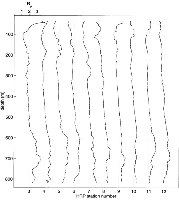
The NATRE site rests within the Central Waters of the North Atlantic sub-tropical gyre (figure 2.1). Several studies (Schmitt and Evans 1978; Schmitt 1981; Schmitt 1990) have argued that salt fingers contribute to the vertical mixing in this region. In particular, these studies argue that finger mixing should dominate turbulent mixing if R, < 2. Indeed, this describes the density ratio structure in the upper 500 m of the NATRE site thermocline (figure 2.2). However, no per-manent thermohaline staircase occurs at the NATRE site. This suggests that the finger contribution to the vertical buoyancy-flux is insufficient for maintaining a series of well mixed layers and sharp interfaces. If turbulent fluxes produced by shear instability of internal waves are large enough (and frequent enough) to over-come the finger fluxes, the net density-flux may be down-gradient. Polzin (1996) has found a clear connection between mixing and shear instability at the NATRE site. His work indicates that exceptional dissipation generally occurs when the local Richardson number (Ri = N2U;-) becomes less than unity. To what extent2
Madeira NATRS HRP Survey Canary Islands Afic 20*N --- --- --350W 30"W 250W 200W 150W 100W
Figure 2.1: Location of the NATRE HRP survey. Over 150 dives were completed over 26 days. The survey consisted of the 100 station grid spanning the (400 km)2
region shown. -An additional 50 stations were tightly centered about (260N,
-28*W). The HRP survey was completed two weeks prior to the tracer-release phase of the experiment.
be explored further.
Despite the lack of a thermohaline staircase, optical structures recorded dur-ing two shadowgraph profiles give qualitative evidence of salt-fdur-inger activity. Thin filament-like optical structures (figure 2.3) occurred from the bottom of the mixed layer (z ~ 150 m) to the base of the thermocline (z - 1000 m). These features
are most abundant just below the mixed layer, occurring in patches with several meter vertical extent, with gaps between patches of 5 to 10 m. Patches containing filament structures become more sparse at at greater depth, but generally occur with a frequency of 2-4 patches for every 40 m. While all possible orientations were encountered, filaments in the form of laminae tilted 10 to 20 degrees from hori-zontal were most frequently observed (figure 2.3a). These structures are identical to those previously observed by Kunze et al. (1987) in a thermohaline staircase. As was the case with the staircase observations, the laminae at the NATRE site are characterized by cross-filament wavelengths of 0.5 to 1 cm. Kunze (1990) identified these structures as salt fingers that have been tilted by shear. Other classes of optical structures observed include sharp interfaces, isotropic features, and billows.
We regard the abundance of thin tilted laminae at the NATRE site as sugges-tive evidence for salt fingers. To quantitasugges-tively assess the frequency and strength of salt fingers at the NATRE site, we rely on estimates of X and E derived from HRP microstructure measurements.
2.3
Quantitative Assessment of Salt-Finger
Mixing
2.3.1
Description of Data
Data from the NATRE HRP survey will provide the foundation for this study. However, with the intent of making our study more general, we have supplemented the NATRE data with data from a second HRP Survey. These data come from field work conducted in the northeast subtropical Pacific at Fieberling Guyot. Data from the Fieberling survey (TOPO) is discussed by Toole et al. (1997a) and Kunze and Toole (1997). In the present study, TOPO data are included as
R p 1 2 3 I I I 100- 200-300 E 400 - 500- 600- 700- 800-3 4 5 6 7 8 9 10 11 12 HRP station number
Figure 2.2: A section showing 10 profiles of the density ratio, R= a < E) >
(# < S, >)-1. The gradients were calculated using a 5-m scale, smoothed using a 50-m running average. Stations 3-12 comprise the meridional section at the western edge of the survey. Each successive station is offset two R, = 2 units and the reference value R, = 2.0 is shown for each profile. There is large variability in the mixed layer and beneath z = 600 m due to intrusive features.
b
Figure 2.3: Shadowgraph images of optical microstructure that were obtained during the NATRE HRP survey. (Shadowgraph image intensity is proportional to the Laplacian of the refractive index of light. The negative of each original image is shown here.) The tilted laminae shown here are observed throughout the thermocline. The circular window has a diameter of 10 cm, and the optical features have a characteristic wavelength of 0.5-1.0 cm. Laminae tilted 10 to 20 degrees from the horizontal (a) were the most frequently observed orientation, although filaments with vertical alignment (b) were also observed. The images shown here were obtained near 300-m depth.
-a me-ans of introducing d-at-a from -a double-diffusively st-able (here-after, doubly stable) stratification regime. While dissipation occurring in the salt-finger regime may be attributable to a combination of turbulence and fingers, dissipation in the doubly stable regime can only be attributed to turbulence. By regarding the features of turbulent dissipation in the doubly stable regime as a null hypothesis, we can objectively assess the dissipation observed in finger-favorable data.
The profile data from NATRE typically extends to 2000 m. These profiles are characterized by a deep mixed layer (80-150 m thick) capping the finger-favorable thermocline. Below the thermocline, intrusive features exist with both "diffusive" favorable (the form of double diffusion with cold-fresh water over warm-salty) and doubly stable character. The TOPO data can be broken into two classes. The data collected above the seamount summit are characterized by high shear and weak stratification in the presence of thermohaline interleaving. The data collected on the seamount flanks are characterized by lower levels of shear and stronger stratification. In particular, these two classes have heterogeneous shear statistics, with shear levels at the summit exceeding those at the flank by a factor of two. For this reason, we will treat these two classes of TOPO data separately in the analysis that follows. While the stratification at the TOPO site was generally doubly stable, some double-diffusive favorable patches were also present.
Initial processing of all HRP data results in estimates of all conventional (e.g., 6, S, U, V) and microstructure quantities at 0.5-m intervals. A detailed descrip-tion of the algorithms used for this initial stage of data analysis can be found in Polzin and Montgomery (1996). Dissipation rates are calculated from observa-tions of thermal and velocity microstructure using the relaobserva-tions X = 2K(302) and
e = v(15/4)(u2 + V), where K and v are the molecular values of thermal diffu-sion and viscosity. The factor of 3 in the x expression and the factor of 3.75 in the c expression come from an assumption of small-scale isotropy. Observations supporting the isotropy relations have been made for turbulence (Yamazaki and Osborn 1990) as well as salt fingers (Lueck 1987). Numerical simulations of salt fingers also indicate isotropy for the thermal gradients (Shen 1995). We note that shadowgraph images associated with fingers show significant structural coherence at O(1 mm) scales. Since the shadowgraph measures the Laplacian of refractive in-dex, the images tend to emphasize the smallest scales which are mainly influenced
by salinity microstructure (Kunze 1990). Thus, small-scale thermal gradients may adhere to the isotropic relationship, while anisotropic salinity structures bias the shadowgraph images.
Finestructure gradient quantities, particularly R, and Ri, will be used exten-sively in the analysis that follows. To estimate the vertical gradients of scalars, we have used the slope of a linear fit over a 5-m segment, centered at each 0.5-m interval. The 5-0.5-m scale was chosen as a suitable trade off between the need for high vertical resolution and statistically reasonable regression estimation. The magnitudes of all 5-m scalar gradients were compared to their associated standard error. Gradient quantities with standard errors larger that twice their magnitude were excluded from the analysis. This resulted in roughly a 5% data loss, mostly from noisy N2 estimates. Figure 2.4 shows typical profiles from the two HRP
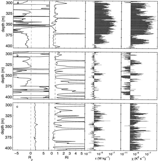
surveys used for this study. Data from the TOPO survey are shown in figure 2.4a (a seamount summit profile) and figure 2.4b (a seamount flank profile). A profile from NATRE is shown in figure 2.4c.
2.3.2
The Dissipation Ratio Model
Mixing by turbulence and salt fingering has traditionally been modeled by the production-dissipation balances for thermal variance (Osborn and Cox 1972) and TKE (Osborn 1980). These balances, in a form relevant to the average over an ensemble of many patches (denoted by < - >), are given by
(1 - Rf)(-k, < N2 >) +Rf <c >=
0, (2.1)
2(-ko < 82 >)- < 8, > + < x >= 0.
(2.2)
In these expressions, N2 and 02 are the vertical gradients of buoyancy andpoten-tial temperature, k, and ko are the vertical eddy diffusivities of buoyancy and tem-perature, and Rf is the mixing efficiency. The mixing efficiency, or flux Richardson number, dictates the fraction of Reynolds stress production that is converted to potential energy flux (i.e., Rf = -k, < N2 > (u'w' < Uz >)- ).
C-_
-
n- ---1 -...- 7. 5 0 1 2 3 4 5 10-11 o-9 10-7 Ri E (W kg~1) 10-1 10~9 10-7 X (K2s-1)Figure 2.4: Characteristic profiles of RP, Ri, E and x from the three HRP data groups used in this study. (a) Data from above the summit of Fieberling Guyot collected as part of the TOPO HRP survey. (b) Data from the flank of Fieberling Guyot, about 20 km off the axis of the summit. (c) Data from the NATRE HRP survey. The TOPO site is characterized by predominantly doubly stable stratification (R, < 0). In each profile of Ri, a reference value of 0.5 is shown as the dashed vertical line. The high occurrence of low Ri above the seamount distinguishes the summit profiles (a) from those above the seamount flanks (b).
E - 350 0. a> -o 300 325 E 5 350 375 400 300 325 - 350 375 400 -5 0 R p
-k, < N2 > = g (a(-ko <
8z >)+ 3(-k, < S
>))
= g a(-ko < 8z >)(1 - r-().
where we have defined the heat/salt buoyancy-flux ratio r = (ko/k,)R,. In all
cases, vertical scalar fluxes have been written in a Fickian form, with the eddy diffusivities being positive for down-gradient flux. Furthermore, we have carried a separate diffusivity for each scalar. In the case of salt fingering, not only do we expect the diffusivities to be different, but also that the salt flux can dominate the buoyancy flux so that k, <0.
A general relation involving the ratio of thermal and buoyancy diffusivities can be derived using (2.1), (2.2) and (2.3) with N2 = gaO8(1
-R,), F = {(R i
1-R k (2.4)
Rf (Rp-1 r r *
1-R5) Rp) r-1'
The nondimensional parameter F (Oakey 1985) is the scaled ratio of the dissipa-tion rates,
< x >< N2 >
F = .(2.5)
2 < c >< E)z >2*
We will refer to F as the "dissipation ratio", although it has been referred to as "the mixing efficiency" by many investigators. While F is related to the mixing ef-ficiency, it is more generally related to the ratio of heat and buoyancy diffusivities. Oakey (1985) considered the case of turbulent mixing and derived
rM = R f (2.6)
1 - Rf
This expression can be obtained from (2.4) by setting ko = kP, so that r = R,.
The superscript (t) is used to denote that the relation is valid when turbulence is the sole dissipative mechanism. Thus, within the context of turbulent mixing, the dissipation ratio is related in a simple manner to the mixing efficiency Rf . We note that expression (2.6) can be restated as FM = (k, < N2 >)/ < E > . Therefore,
while Rf is the ratio of potential energy gain to kinetic energy input, 17M is the ratio of potential energy gain to kinetic energy loss. Laboratory experiments have demonstrated that the mixing efficiency of turbulence is small, with estimates
ranging from Rf = 0.05 (Huq and Britter 1995) to Rf = 0.20 (Rohr et al. 1984). In terms of the oceanographic application of (2.1), p(t) = 0.2 is often used (Moum 1996).
Hamilton et al. (1989) and McDougall and Ruddick (1992) considered the case of salt-finger mixing and derived
(f) ( R- 1 -1 r (2.7)
with the superscript (f) used to denote dissipation by salt fingers. This expression is also a special case of (2.4) where the Reynolds stress production (P = u'w'U2)
is zero such that limpro Rf (1 - Rf )- = -1, as is the case for convection with
a TKE balance of -kp < N2 >=< c > .
Thus, for salt-finger mixing, F is (minus) the ratio of the thermal to buoyancy diffusivity (i.e., (f) = -ko/k,).
The size of this ratio is set by both the density ratio and the buoyancy-flux ratio of the fingers. The plausible range of the buoyancy-flux ratio r is known from theory (Stern 1975; Schmitt 1979a), laboratory work (Turner 1967; Schmitt 1979b; McDougall and Taylor 1984; Taylor and Bucens 1989), and numerical simulations
(Shen 1993,1995). This collection of work suggests 0.4 < r < 0.7.
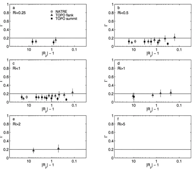
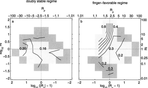
Figure 2.5 presents the plausible range of the nondimensional parameters of the salt-finger and turbulence models. Results from laboratory studies were used to plot the mixing efficiency of turbulence (5a) and the buoyancy-flux ratio of salt fingers (5b). These numbers were used to compute the dissipation ratio models for turbulence and salt fingers (5c). The value ](t) = 0.2 is shown as representative of the turbulence model, with a plausible range shown as 0.05 < 00 < 0.25. The plausible range of the salt-finger dissipation ratio is shown with a 99% confidence band determined from the density-ratio binned statistics of r.
2.3.3
Method of Analysis
Our primary investigation of the dissipation rates will be done using the dissipation ratio F. The existence of simple models for F in cases of turbulent and salt-finger dissipation give this parameter merit. However, two issues detract from this parameter's apparent usefulness. First, differences as small as a factor of two distinguish the value of F between the two processes. This obstacle can be
C 0.8 o 0.6 C E 0.4 0.2 0 b X 0.8 &A AA 60.6-0U 0.4 4 Tumer 67 02eSchmitt 79
McDougall and Taylor 84 M Taylor and Bucens 89
0 C fingers S0. 8 0 06 0.4 ~ .4 0 0.1 1 10 R -1 p
Figure 2.5: The plausible range of three nondimensional parameters for finger-favorable stratification (R, > 1). The logarithmic axis for R, - 1 is useful because the distribution of finger-favorable R, is approximately lognormal about R, = 2. (a) The mixing efficiency of turbulent mixing (Rf ). Laboratory data supports the range 0.05 < Rf < 0.20. (b) The buoyancy-flux ratio of salt fingers r from laboratory data. (c) The range of the dissipation ratio for turbulence and salt fingers are shown. The turbulence model was calculated using IN) = Rf (1
-Rf )-1, with p(t) = 0.2 taken as the nominal value. The finger model was computed
from the laboratory data for r, with average values of r binned by RP. The 99% confidence band is shown for the finger model while the range for the turbulence model is dictated by 0.05 < Rf < 0.20.
overcome by incorporating large numbers of dissipation observations into each estimate of F to reduce error bars enough to resolve such a subtle parameter range. This is a serious consideration since F is the ratio of four noisy variables. Second, given an ensemble of dissipation observations, only a fraction of the data may be representative of mixing events appropriately modeled by (2.1) and (2.2). This issue must receive careful attention.
The dissipation rates c and x are computed by integrating the observed shear and thermal variance residing at scales between about 1 and 50 cm. Variance at these scales originates from diabatic, irreversible processes. The processes of turbulence and salt fingering are among these, producing fluxes of heat, salt, and buoyancy that irreversibly alter the local temperature, salinity, and density finestructure. However, it is plausible that internal wave and molecular processes may also account for variance at small enough scales to influence dissipation esti-mates, and these set the oceanic background levels of the dissipation rates. This type of oceanic "noise" is not appropriately modeled by (2.1) and (2.2). Similarly, the noise of the sensors and associated electronics, though low for the HRP (Polzin and Montgomery 1996), will contribute to uncertainty in E and
X-In the work presented here, we seek to attribute observations of irreversible microstructure to salt fingers or turbulence. We have attempted to rule out the influence of noisy dissipation estimates by only examining dissipative events of higher magnitude, while still retaining enough data to uncover a potentially subtle signal of salt fingers. To do this, we have used the combined data set involving observations from both NATRE and TOPO surveys. This combined dissipation record was then examined in terms of various upper thresholds of dissipation rate magnitude, this being done separately for observations occurring in doubly stable and finger-favorable patches.
We have found that exceptional levels of finger-favorable X are associated with bimodal E statistics. In particular, we have examined the distribution of E data using a threshold defined as X > X75 ~ 1 x 10⁻⁹ K2S-1 : the upper 75 percentile
of the combined x record. The statistical distribution for E(X > X75) is shown in figure 2.6. The finger-favorable data (figure 2.6a) seems to have a primary mode at
E 2 x 10⁻¹⁰ W kg-1 with the secondary mode occurring near 1 x 110-9 W kg- 1.
antimode at c - 5 x 10⁻¹⁰ W kg-1 is significant to the 0.15 level (i.e., significant at the 85% confidence level). In contrast to the finger-favorable data, the associated distribution of doubly stable c data lacks bimodal character (figure 2.6b). Both turbulence and salt fingers act as dissipative mechanisms in the finger-favorable regime, while only turbulence acts in the doubly stable regime. The existence of bimodal c in only the finger-favorable regime suggests that the two modes are associated with the two processes.
To investigate the character of the finger-favorable data more thoroughly, we have examined the E(X > X75) population in terms of the stability parameters R, and Ri. Figure 2.7 shows the distribution of E(x> X75) data after being partitioned into four subsections of (Rp, Ri) data space. When the portion of parameter space having Ri > 1 is considered, the low-e mode dominates. This is particularly true when R, < 2 (figure 2.7a), this low density ratio range having about twice the number of E(x > X75) events as R, > 2 (figure 2.7b). In the portion of parameter space with Ri < 1 (figures 2.7c and 2.7d), the high-e mode is apparent at both large and small values of R,. However, in the case where (1 < RP < 2, Ri < 1), a low-E mode is also apparent, with a population comparable to the high-e mode. The documented trend is consistent with an association of the two modes with turbulence and salt fingering. In particular, we associate the low-e mode, dominant at low RP, with salt fingers. We associate the high-e mode, dominant at low Ri, with turbulence.
Ruddick et al. (1997) used microstructure observations from a different in-strument to examine dissipation at the NATRE site. The noise level of their measurements limited their analysis to observations having E > 7 x 10- W kg- 1.
Their observations clearly fall into the high-c mode that we have associated with turbulence. Ruddick et al. (1997) use a Reynolds number, Re = e/(vN2), and
they find no clear evidence of salt fingers in the parameter range 101 < Re < 104.
In a salt-finger regime, the parameter c/(vN2
) is equivalent to the Stern number,
Jb/(vN2). Stern (1969) argued that this parameter must be 0(1) for fingers to be active, while McDougall and Taylor (1984) found experimentally that the Stern number can be 0(10) for R, < 2. A characteristic Stern number for our low-c mode is 0(10). Thus, the Ruddick et al. (1997) Reynolds numbers are too large to admit the possibility for fingers.