HAL Id: hal-01113230
https://hal.archives-ouvertes.fr/hal-01113230
Preprint submitted on 5 Feb 2015
HAL is a multi-disciplinary open access
archive for the deposit and dissemination of
sci-entific research documents, whether they are
pub-lished or not. The documents may come from
teaching and research institutions in France or
L’archive ouverte pluridisciplinaire HAL, est
destinée au dépôt et à la diffusion de documents
scientifiques de niveau recherche, publiés ou non,
émanant des établissements d’enseignement et de
recherche français ou étrangers, des laboratoires
Residential Space Heating Determinants and
Supply-Side Restrictions: Discrete Choice Approach
Elena Stolyarova, Hélène Le Cadre, Dominique Osso, Benoit Allibe, Nadia
Maïzi
To cite this version:
Elena Stolyarova, Hélène Le Cadre, Dominique Osso, Benoit Allibe, Nadia Maïzi. Residential Space
Heating Determinants and Supply-Side Restrictions: Discrete Choice Approach. 2015. �hal-01113230�
Residential Space Heating Determinants and Supply-side Restrictions: Discrete
Choice Approach
Elena Stolyarova1,2,∗, H´el`ene Le Cadre2, Dominique Osso1, Benoit Allibe1, Nadia Ma¨ızi2
Abstract
This paper provides an empirical analysis of the supply-side constraints that impact household choices of space heating systems in French dwellings. Based on data from the 2006 National Housing Survey and the 2013 Household Survey, we estimate discrete choice models using socio-demographic, dwelling and spatial characteristics as determinants of choice. In order to capture the supply-side constraints, we perform a post-estimation clustering based on the Expectation-Maximization algorithm, which allows us to determine the groups of households that are most likely to choose each considered space heating system. The results suggest that for 2006, households living in individual houses preferred to heat space using an individual boiler, whereas those living in apartments opted for direct electric heating. In 2013 all households preferred direct electric heating, and wood heating became their second choice. The discrete choice models do not show a significant change in behavior from 2006 to 2013. The post-estimation clustering indicates that many households were strongly constrained by the conditions and characteristics of their living space in 2006. The mean probability of choosing direct electric heating or a boiler was more than 0.8 for 21% of households living in houses and for 36% living in apartments. Thus, these households did not seem to have a choice. In 2013 the supply-side constraints were weaker. The highest mean probability (0.755) is observed in the group opting for an individual boiler. We also observe an increase in the popularity of heat pump and wood heating systems.
Keywords: Dwelling Energy choice, Household Behavior, Multinomial Logit, Space Heating Systems
JEL:C25, C46, D12, D19, Q40, Q55
1. Introduction
French residential consumption represents a significant 26.5% (including wood) of total final energy consumption, which stood at 154.4 Mtoe3 in 2013 (ADEME, 2014a). The largest share of this consumption, between 50% and 70% on average, is used for space heating (ADEME, 2014a). The French government set a target to reduce energy consumption in the building sector by at least 38% from the 2006 baseline by 20204. To achieve this target, two measures have been introduced into the residential sector: the new thermal regulation oversees energy efficiency retrofit measures and the government has created several types of financial aid to encourage households to undertake retrofit work. Despite these measures, energy consumption is decreasing too slowly: a drop of 2.6% in 2013 and only 1.4% from 2000 to 2010 (ADEME, 2014a; CEREN, 2011). French residential statistics show that dwellings built prior to the first thermal regulation of 1974 represent the most significant energy-saving potential. According to ADEME5, dwellings built before 1974 account for 55% of building stock and consume 64% of total residential energy consumption, while those built after 1998 account for 16% and represent only 11% of energy consumption. However,
∗
Corresponding author
Email address: [email protected] (Elena Stolyarova )
1EDF R&D, ENERgie dans les BAtiments et les Territoires, av.des Renardi`eres Ecuelles, 77818, Moret sur Loing, France 2MINES ParisTech, PSL Research University, CMA, CS 10207 rue Claude Daunesse, 06904, Sophia-Antipolis, France 3Million tons of Oil Equivalent.
4SOeS
part of this potential remains underexploited for two main reasons, i.e. slow increase of building stock, at only +1% new dwellings per year, and low level of retrofit works, which are insufficient to reduce energy consumption to meet an ambitious target of a 38% reduction in energy consumption in the building sector6.
To improve this situation, it is important not only to understand the main drivers of household behavior concerning energy consumption in the dwelling, but also to identify which supply-side barriers to overcome. For example, dwellings do not always have access to all energy sources. Natural gas can only be used in buildings connected to the grid, so that dwelling that is not located close to the gas pipeline requires major financial investment. Only 28% of French municipalities7and 49.8% of dwellings had access to the gas grid in 2006 (INSEE, 2006). Wood heating is usually used in individual houses with free and ready access to wood. Moreover, fuel oil, wood and liquefied petroleum gas (LPG) need space for storage. Households cannot instantly switch from one source to another because Residential Space Heating Systems (RSHS) and domestic hot water generally use a single energy. A household that wants to change energy source must therefore buy and install new equipment. The dwelling occupation status, i.e. owner or tenant, also impacts possible retrofit actions.
The contribution of this study to the existing discrete choice framework on the determinants of residential energy behavior is threefold. First, we analyze space-heating determinants from the perspective of the socio-demographic, dwelling and spatial barriers that need to be overcome, since households cannot instantly change these characteristics. Second, we use post-estimation clustering to try to determine the household groups for which the degree of supply-side constraints is the highest. Le Cadre et al. (2009) propose to use the distribution of individual estimated probabilities from a discrete choice model in order to divide the population into groups. Following the same logic, we carry out a post-estimation clustering based on an Expectation-Maximization algorithm in order to determine which households prefer which heating system. Finally, we compare two years and analyze the change in supply-side constraints.
The rest of this paper is organized as follows. We offer a brief literature review on the discrete choice approach in Section 2. Section 3 describes the econometric approach and methodology for unsupervised clustering, followed by section 4 in which we present the model specification. The data and some descriptive statistics are presented in Section 5. In Section 6 we provide the estimation results for the choice of RSHS. Section 7 presents the results of post-estimation clustering. Finally, some concluding remarks are made in Section 8.
2. Literature review
In this study, we concentrate on micro econometric analysis, especially discrete choice models, which aim to display, predict and explain the choice between two or more mutually exclusive discrete alternatives. We can group recent works that use a discrete choice approach in the energy sector into 3 subjects.
The first type of study analyzes the impact of the consumer situation (socio-demographic, dwelling and spatial characteristics) on choices related to energy topics in dwellings. For example, Scasny and Urban (2009) investigate the impact of socio-demographic and dwelling characteristics on the presence or absence of various appliances in the home, such as dishwashers, fridges and microwaves in OECD countries. They also try to determine the number of appliances by type and the household energy-saving activities. Ameli and Brandt (2014) attempt to determine the social characteristics and behavior attitudes that explain the decision to invest in energy efficiency equipment (light, appliances, RSHS) and retrofit work. Ricci and B´erang`ere (2014) investigate which household conditions push French energy-vulnerable consumers into fuel poverty. Michelsen and Madlener (2012) analyze the influence of RSHS attributes and household situation on the decision to adopt innovative residential heating system. Braun (2010) proposes a space-heating choice model for Germany that focuses on dwelling types and regional differences. Rahut et al. (2014) examine the impact of socio-demographic variables on the choice of energy source in Bhutan.
The second type of article looks at the level of expected energy consumption, which is estimated simultaneously by discrete choice models and linear regression models. This framework, called discrete-continuous choice models, was proposed by Dubin and McFadden (1984), who at the same time investigate the demand for appliances and the demand for electricity by appliances. Using the same type of model, Nesbakken (1999), Vaage (2000) estimate fuel energy choices and consumption in Norway. Couture et al. (2012) look at wood-space heating choices and consumption in
6French Ministry of Ecology, Sustainable Development and Energy 7GDF Suez
the French Midi-Pyrnes region. Mansur et al. (2008) estimate an American energy model to determine the choice and consumption of fuel oil in buildings by both households and firms. They take into account the impact on climate. Liao and Chang (2002) investigate the energy demand for space heating and domestic hot water uses in the United States with a focus on old people.
Lastly, the third type of study use stated preferences data from a choice experiment survey. This data type is subject to a wide range of economic interpretations (e.g. willingness to pay, reservation prices, consumer surplus, etc.). Moreover, researchers can use this data to obtain information on alternatives not chosen by consumers and on alternatives that do not yet exist. Islam and Meade (2013) study the conditions for photovoltaic adaptation by Canadian households. Achtnicht (2011), Achtnicht and Madlener (2014) analyze how environmental benefits impact the choice of heating system and retrofit works in Germany. Banfi et al. (2008) estimate consumers willingness to pay for energy-saving measures in Swiss residential dwellings for both tenants and owners. Rouvinen and Matero (2013) perform stated choice experiment on private homeowners choice of heating system in Finland. The results show that Finnish households prefer ground-source heating and district heating, and that existing heating systems and dwelling characteristics have a significant impact on choices.
3. Methods
3.1. Discrete choice framework
The discrete choice approach, or Random Utility Model (RUM), was initially proposed by Thurstone (1927) and later adapted to economics by McFadden (1974). The RUM is composed of two parts. One is observable by the researcher and can be estimated, the other is considered to be random. The RUM allows us to obtain the probability by choice alternative and by household. The utility function for choice j among J mutually exclusive choice alternatives on N households can be described as:
Ujn= Vjn+ ξjn, ∀n =1, ..., N, ∀ j = 1, ..., J (1)
Where Ujnis the utility of choice j for household n, Vjnis the determinist part of utility observable by the researcher, and ξjn is a stochastic random variable comprising unobservable household and dwelling characteristics, as well as measurement errors. To estimate the determinist part of utility, the researchers suppose Vjnto be linear in parameters:
Vjn= βTXjn (2)
The vector of unknown parameters to estimate is expressed in β where T stands for the transpose operator. Xjn represents the matrix of explanatory variables. In this study we decided to use a standard Multinomial Logit Model (MNL) where ξjnis independent and identically distributed following the Gumbel Extreme Value distribution. The density function f (.) and the cumulative distribution function F(.) for each unobserved component of utility:
f(ξjn) = e −π2 6e−eξ jn (3) F(ξjn) = e −eξ jn (4) The difference between two Gumbel variables gives a logistic distribution:
F(ξjn− ξin) =
eξjn−ξin
1 + eξjn−ξin (5)
The probability that household n chooses choice alternative j is inferred from equation 5 given by a closed form expression in equation 6 and fitted by Maximum Likelihood estimation.
P(ξjn) = eβTX jn PJ i=1eβ TX in (6) The estimated parameters give us the impact of the explanatory variables on the probability of choosing one choice alternative compared to the reference (or base) alternative and to the reference level of categorical variable. The use of MNL was also spurred by the nature of the dataset, which only allows us to estimate alternative specific individual parameters. Note that both datasets are revealed preference data, i.e. we know the final choice or situation of households but we have no information about the characteristics of the alternatives not chosen.
3.2. Methodology for unsupervised clustering
Assuming that the estimated probability distribution is a Gaussian mixture, we can use the Expectation-Maximization (EM) algorithm to cluster the households into groups. The EM algorithm was proposed by Dempster et al. (1977). This is a two-step algorithm. In the first step, we compute the expected value of the log likelihood function (normal distribution function in our case). In the second step, maximization, we find the parameters of distribution that max-imize the log likelihood quantity. To perform the clustering we use a mclust package for R (Fraley et al., 2012). For univariate data, as in our case, the package proposes two types of Gaussian mixture, i.e. with equal variance for all normal distribution in the mixture, and different variance for each distribution. The number of classes for clustering and the type of mixture are chosen in order to minimize the Bayesian Information Criterion (BIC) (Schwarz, 1978). 4. Model specification
The concept of household choice of RSHS is complicated and depends on the households situation. A household can choose the type of RSHS and energy source at the time of construction if it is buying a new dwelling. In this case, the household is limited only by its income, preferences and access to energy sources. Alternatively, a household can choose the RSHS indirectly at the time of purchase (owner) or when signing the rental contract (tenant). However, in the case of social tenants (HLM8or other), households do not choose their dwelling, which in France is allocated by a commission for each HLM body after analyzing households situations. Once an RSHS has been installed, it is difficult to change its type. Boilers, district heating, air/ water and water/water heat pumps require water loop networks. Direct electric heating requires radiative, convection or other types of heater. Wood heating systems (chimneys, wood burning stoves, etc.) need space to store wood and a network for hot air distribution in all dwelling. These network costs add to the cost of RSHS installation.
We must also consider who takes the decision to perform retrofit work in dwellings. In individual houses, owners decide to initiate retrofit work, either for themselves or their tenants. In the case of co-owned dwellings, all owners need to make the decision. In France, the average duration, from the point when co-owners decide to undertake space heating work to the point when the work is completed, is estimated at 4 to 5 years (ADEME, 2014b). Finally, we must point out the importance of household preferences at the time of choosing an RSHS, such as: energy type, type of heater, product brand, cost, government grant, information about RSHS type, etc.
The age of dwelling seems to be an important determinant in household choices. The French government has raised thermal standards for buildings since 19749. The level of insulation also impacts on choice because energy bills are higher in dwelling with no insulation than in insulated dwellings. Household size is correlated to dwelling size, and thus increases annual space-heating bills. In order to separate the effect of dwelling size from household size, we use both variables as determinants of choice. The absence of access to the gas grid limits household choice for fuel used in boilers. The use of fuel oil and LPG in boilers is costly, and electric and wood boilers are not widespread. Therefore, if households do not have access to the gas grid, the likelihood of installing a boiler decreases.
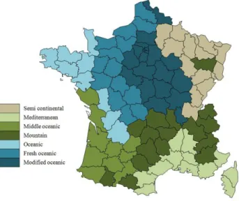
To take into account the climate variability in France, we decided to use the climate zone as an explanatory variable. Another possible option is to use the normalized heating degree days by French d´epartment. However, this measure focuses exclusively on the outdoor temperature. Other climate characteristics can impact the choice of RSHS, such as: the level of precipitation, the cycles and rhythms, number and duration of extreme events per year (storm, snow, heatwave, etc.). Households may also choose the location of their residence in line with individual climate preferences. We integrate into our model 7 climate zones as defined in the National Housing Survey (2006): oceanic, fresh oceanic, middle oceanic, modified oceanic, semi-continental, Mediterranean and mountain (Figure 1). As the climate zone does not consider the landscape of the residential area, we introduce urban density as a determinant of choice. Dwellings in rural zones have easier access to wood, but more difficulties accessing the gas grid.
Energy prices and the cost of space-heating installation also affect household choice. The data type used in our study does not give us information about the age of RSHS and we cannot propose an approximate cost of installation due to high variation of installation costs (Laurent et al., 2011). Moreover the mean costs for each type of RSHS are
8Rent-controlled housing (in French: Habitation `a Loyer Mod´er´e)
Figure 1: Climate zone location as defined in NHS 2006 (INSEE, 2006)
not the same from one database to another (Laurent et al., 2007). To input energy prices into the models, we assume that the heating system is chosen when the household moves into a new dwelling.
Finally, socio-demographic factors can impact household choice. We use only income level in our estimations. We tried to implement other social and economic characteristics: social professional category of household reference person and his/her partner, highest level of education, main occupation (employment status, student, pensioner, etc.). However, these are not significant for two reasons: first, these characteristics tend to evolve from year to year, whereas the energy choice covers a longer period; second, these characteristics are correlated with the occupancy status, income level, size of dwelling and the age of the household reference person.
In our study we use Revealed Preferences data, which only gives us information about the RSHS chosen and a description of the household situation. We propose to consider the households’ situation at the time of the surveys as a result of consecutive choices. These results can be summarized by the final situation: household dwellings possess accurate RSHS. Households are assumed to have chosen the situation that maximizes their utility with respect to their income, the characteristics of the dwelling and energy prices. Thus, we can investigate the impact of the household environment on their dwelling space heating profile. We consider the most common, widespread heating system in France: space heating by Direct Electric Heating (DEH) and boiler (individual or collective). We also add the choice of a heat pump and wood heating system (chimney, wood burning stove) to take into account systems based on renewable energy.
5. Data
To analyze the year 2006, we used the most recent National Housing Survey (NHS 2006) published by INSEE10 which describes French housing expenditure and household living conditions (INSEE, 2006). The NHS 2006 is a large survey11 covering 42,701 main residences. The survey provides detailed data on building characteristics, household living conditions (legal measures for occupation, difficulties in access to housing, household residential mobility, etc.), energy expenditure and consumption of wood. We can clearly identify the energy source for different uses and the type of heating system. We were forced to reduce the dataset from 42,701 to 32,305 dwellings due to lack of information on energy expenditure, consumption and RSHS for French overseas territories. We also removed dwellings with minority heating systems that are not part of our study. We took out dwellings that were neither houses nor apartments, and those for which the housing occupancy status was neither owner nor tenant.
10French National Institute for Statistics and Economic Research (in French: Institut National de la Statistique et des ´Etudes ´Economiques) 11The next NHS is scheduled for 2016
The second dataset is a 2013 Housing Survey (HS 2013) conducted by TNS SOFRES on behalf of EDF12 and covering 1,350 main French residences after data clearing. The HS 2013 data is a detailed survey covering energy ex-penditure, energy equipment for home end-uses, appliances, lighting, energy consumption, electricity tariffs, dwelling and household characteristics.
We also used an additional dataset of energy prices (in euro at current prices) by dwelling characteristic and by year from 1983 to 2006. Energy prices were taken from a French database P´egase (Minist`ere de l’´ecologie, du d´eveloppement durable et de l’´energie, 2014). As we are examining the choice of RSHS, we take the tariff correspond-ing to high energy consumption. We choose 3 in and off peak rates for electricity: the price for small apartments13 with 6 kVA power, the price for other apartments with 9 kVA power and the price for individual houses with 12 kVA power. For natural gas, we consider the rate for apartments and the rate for houses. For fuel oil we do not have much choice, because the P´egase database only gives the rate for individual houses. The price is given in euro by 100 kWh for electricity, and by 100 kWh LCV14for natural gas and fuel oil.
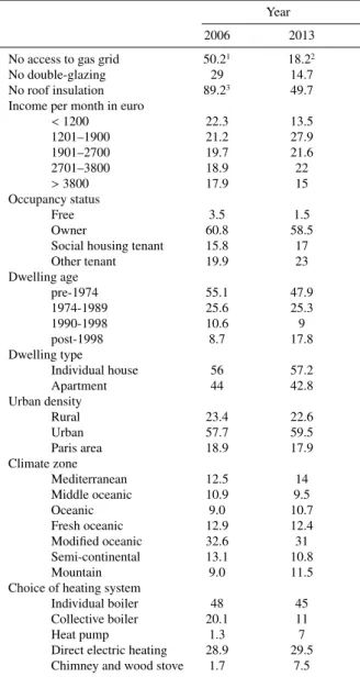
The descriptive statistics of choice determinants are given in Table 1 and Table 2. The map of climate zones is displayed in Figure 1. Access to the gas grid and roof insulation are not comparable between the two datasets. HNS 2006 gives us information on access to the gas grid for each dwelling, but HS 2013 only provides information on towns access to the gas grid. There are 36,614 municipal areas in France, 72% of which do not have access to gas grid. We note that in HS 2013, only 18.2% of municipal areas have no access to the gas grid. This percentage is explained by the design of the survey.
12Electricit´e de France
13Small apartment - apartment with living area under 35 square meters 14Lower Calorific Value
Table 1: Summary of the socio-demographic and dwelling caracterestics Year
2006 2013 No access to gas grid 50.21 18.22
No double-glazing 29 14.7 No roof insulation 89.23 49.7
Income per month in euro
<1200 22.3 13.5 1201–1900 21.2 27.9 1901–2700 19.7 21.6 2701–3800 18.9 22 >3800 17.9 15 Occupancy status Free 3.5 1.5 Owner 60.8 58.5 Social housing tenant 15.8 17 Other tenant 19.9 23 Dwelling age pre-1974 55.1 47.9 1974-1989 25.6 25.3 1990-1998 10.6 9 post-1998 8.7 17.8 Dwelling type Individual house 56 57.2 Apartment 44 42.8 Urban density Rural 23.4 22.6 Urban 57.7 59.5 Paris area 18.9 17.9 Climate zone Mediterranean 12.5 14 Middle oceanic 10.9 9.5 Oceanic 9.0 10.7 Fresh oceanic 12.9 12.4 Modified oceanic 32.6 31 Semi-continental 13.1 10.8 Mountain 9.0 11.5 Choice of heating system
Individual boiler 48 45 Collective boiler 20.1 11 Heat pump 1.3 7 Direct electric heating 28.9 29.5 Chimney and wood stove 1.7 7.5
1The dwelling has no access to the gas grid, but the town may have access. 2The town of residence has no access to the gas grid.
Table 2: Summary of continuous variables
Variables Min Mean Max Std. dev. Electricity price for small flat (Euros/100 kWh) 10.59 15.29 12.51 0.92 Electricity price for flat (euro/100 kWh) 9.84 14.34 11.95 0.83 Electricity price for house (euro/100 kWh) 9.13 14.06 11.31 0.93 Natural gas price for flat (euro/100 kWh LCV) 3.31 7.37 4.42 1.20 Natural gas price for house (euro/100 kWh LCV) 3.06 7.04 4.20 1.18 Fuel oil price for house (euro/100 kWh LCV) 2.80 9.72 4.72 2.03 Number of inhabitants 2006 1 2.3 14 1.27 Number of inhabitants 2013 1 2.16 6 1.11 Living area (m2) 2006 11 93.5 999 46
Living area (m2) 2013 15 97.5 350 41
Age of reference person 2006 16 52.3 101 17.4 Age of reference person 2013 20 52.2 97 16
1The living area is calculated only for dwelling areas above 1.80 meters high.
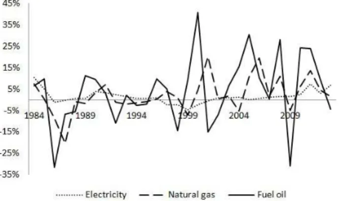
Figure 2: Growth rate of domestic energy prices from 1983 to 2013, P´egase 2014
For the remaining variables, we observe no significant differences between 2006 and 2013 for most dwelling and household characteristics, with three exceptions.
First, the penetration rate of double-glazing increases: 85.3% of dwellings have double-glazing in HS 2013 against 71% in NHS 2006. Next, in HS 2013 the number of dwellings built after 1998 is double that of NHS 2006. This is logical, since by definition, the period ”After 1998” totals 15 years in HS 2013 against 8 years in HNS 2006. Finally, 27.9% of households have a monthly income of between 1,201 and 1,900 euro in 2013, compared to 21.2% in 2006. The share of low-income households (income lower than €1,200) drops from 22.3% to 13.5%. This change can be explained by an increase in the guaranteed monthly minimum net wage in France (S.M.I.C15) from €984.61 in 2006 to €1121.71 in 2013.
More than half of households own their residence, 16% – 17% are social tenants (HLM), about 21% are non-social tenants and about 2% occupy dwelling free of charge. 57% of dwellings are individual houses, the rest are collective (apartments). Dwellings in urban areas account for 77.3%, one quarter of which is located in the city of Paris. One third of households live in modified oceanic climate zones. The average household comprises 2.2 people, with a living area of about 94 square meters. The average age of the reference household person is 52.2. Figure 2 shows the growth rates of domestic energy prices from 1983 to 2013. The price of fuel oil is the most volatile followed by natural gas. The growth rate of electricity prices is more stable, but it follows a similar trend to gas and fuel oil prices.
Regarding the frequencies of choice alternatives for 2006 and 2013, we can see that the number of households using heat pumps or wood as their main energy source for heating increased sharply in 2013 showing the increase of renewable energy use, which reduced the market share of boilers. However, the market share of DEH did not change between 2006 and 2013.
6. Estimation results and discussion
We propose three models to quantify the choice of RSHS: in individual houses (2006), in apartments (2006) and for all dwellings in 201316. All models have the following choice alternatives: DEH (base alternative), heat pump, or individual boiler17. In NHS 2006, we only use collective boilers as a choice in the apartments model, and only use wood heating systems in the individual houses model. However, HS 2013 shows a significant share of collective boilers used in houses and wood-burning stoves in apartments, which cannot be ignored. We therefore use both RSHSs in the same model.
To input the energy prices into the models, we assume that the RSHS is chosen when the household moves into a new dwelling. Only NHS 2006 provides us with information on the year that households moved into their homes. For each household, we take the electricity, natural gas and fuel oil prices for the year they moved in from a database P´egas 2014. Prices are available dating from 1983. This means that the parameters associated with energy prices only impact the choice probabilities for dwelling occupied by the same household since 1983. We try to bridge the lack of information by implementing the mean annual prices for the years before 1983, the growth rate of energy prices, and the same energy prices for dwellings without prices, but none of these configurations works. Moreover if we remove energy prices for all dwellings, the quality of the model decreases.
6.1. Results for both 2006 and 2013 years
The estimation results are given in Tables 3, 4 and 5. The estimation makes a satisfactory adjustment of data with pseudo ¯ρ2 about 0.33 for 2006 models and 0.2 for 201318. The estimation results clearly indicate that the preferred heating system depends on the dwelling type in 2006. Occupants of individual houses prefer to heat space using boilers, while occupants of apartments prefer DEH ceteris paribus. However, the least preferred heating system is the same the heat pump. If we look at the results for 2013, we note that the order of preference has changed. DEH is the preferred heating system for all dwelling types, followed by chimneys and wood burning stoves and ending with collective boilers. Households seem to have no preference between individual boilers and heat pumps when the value of constants is closed: -2.5 for individual boilers and -2.53 for heat pumps.
In 2006, the impact of fuel price is not significant in both models. The level of income, household size and age are not significant in the apartment model 2006. In 2013, income, dwelling occupation status, access to the gas grid and insulation are not significant. For other variables, we observe that an increase in household age and household size increases the probability of using a boiler, heat pump or wood heating in dwellings for both years. However, this impact is limited and the Relative Risk Ratio19(RRR) never exceeds 2 with the highest RRR in 2013: the probability of using a collective boiler or heat pump is multiplied by 1.3-1.4 for each additional inhabitant. We also observe a similarity for climate variables in the model. DEH, heat pumps and wood heating are more prevalent in the Mediterranean climate zone. Wood heating is also a more likely choice in the semi-continental climate.
6.2. Individual houses in 2006
For 2006, the results have two important implications. The absence of access to the gas grid has the highest effect on choice probability in favor of DEH systems. The RRR is 0.03*** for individual boilers in individual houses and 0.014*** for individual boilers (0.07*** for collective boilers) in apartments. This means that if a dwelling has no access to the gas grid, the probability of having a boiler in a dwelling in 2006 was divided by 14–71. The lack of double-glazing multiplies the probability of choosing an individual boiler by 1.91 and of choosing wood heating by 1.637. The absence of roof insulation increases the probability of choosing wood with RRR 1.981***
The energy prices parameters have the expected sign. An increase in electricity prices encourages the use of boilers and wood heating systems and discourages the use of DEH and heat pumps for which electricity is an energy source. An increase in natural gas prices or fuel oil prices has a negative impact on the probability of choosing boilers and wood heating systems respectively. However, the RRR is close to 1 in individual houses for all choice alternatives.
16The size of sample is not sufficient in 2013 to estimate separate models by dwelling type 17Boiler specific to each dwelling
18The 0.2 of pseudo ¯ρ2is equivalent to 0.5-0.6 R2for linear regression models (McFadden and Domencich, 1975, p. 124) 19A relative risk ratio (RRR) of 2 means that one type of RSHS would be twice as likely to be chosen as another type of RSHS.
A 1 €/100 kWh increase in energy prices multiplies (or divides) the probability of using each RSHS by 1-1.13. High-income households prefer boilers and heat pumps, while low-High-income households prefer wood. More tenants use DEH. Boilers and wood are present in houses built prior to the first thermal regulation, whereas heat pumps are present in new dwellings.
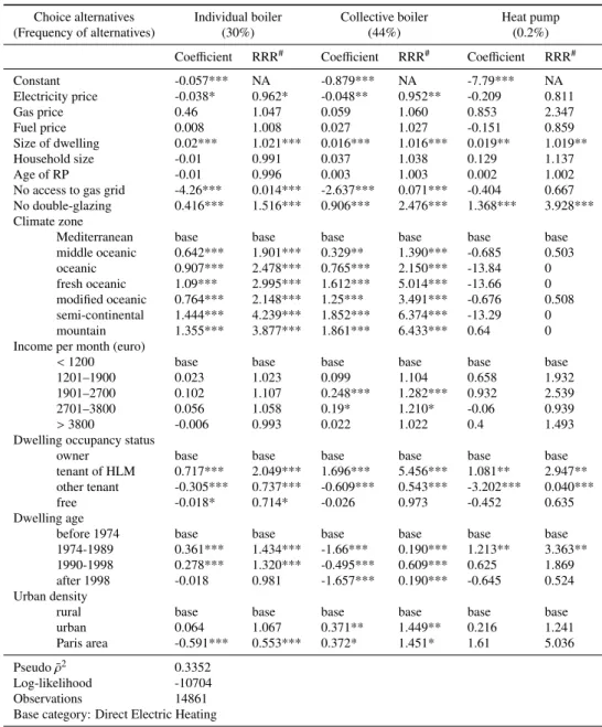
6.3. Apartments in 2006
We observe several differences in the results of heating system choices in apartments (2006). First at all, gas prices, fuel oil prices, size of household, age of referent person and income do not seem to impact on choice probabilities. The coefficient for electricity prices is significant and negative, but has a limited impact on probability, which is divided by 1.23 (RRR 0.811 – 0.962). The size of dwelling increases the probability of choosing a boiler or heat pump, while the presence of double-glazing has a negative impact and encourages the use of DEH. The absence of double-glazing multiplies the probability of using a heat pump by 3.928. Boilers are more prevalent in semi-continental and mountain climate zones. If an apartment is located in a semi-continental climate, the probability of using a boiler is multiplied by 4.239 (individual) or by 6.374 (collective) ceteris paribus. Boilers are mainly present in HLMs with an RRR of between 2.049 (individual) and 5.456 (collective). Collective boilers are used in apartments built prior to 1974: the probability of having a collective boiler is divided by 5 in new buildings. Individual boilers are more prevalent in apartments built between 1974 and 1998. Similarly to the model for individual houses, heat pumps are prevalent in new dwellings. DEH is more widespread than other RSHSs in rural zones, with the exception of Parisian dwellings, where the probability of using an individual boiler is lower than in rural zones and other urban zones.
6.4. Dwellings in 2013
The model for 2013, which includes houses and apartments, reveals some differences. The size of dwelling and household, as well as the age of reference person, are significant and have a positive impact on the probability of choosing a boiler, heat pump or wood with an RRR close to 1. However, double-glazing, roof insulation, occupancy status and income are not significant. As in the 2006 model, heat pumps are most prevalent in the Mediterranean climate zone, while boilers and wood are more common in semi-continental or mountain climate zones. For dwelling built before first thermal regulation (1974), the probability of having an individual boiler, collective boiler or wood heating is divided on average by 2, 10 and 3 respectively. Heat pumps are more prevalent in new dwellings at RRR 1.465. The ”apartment” dwelling type is more likely to have a collective boiler with RRR 51.8.
Table 3: Results of MNL for choice of heating system in individual house (2006) Choice alternatives Individual boiler Heat pump Wood (Frequency of alternatives) (64%) (1.5%) (3%)
Coefficient RRR# Coefficient RRR# Coefficient RRR#
Constant 2.21*** NA -5.817*** NA -0.322*** NA Electricity price 0.0387** 1.039** -0.128*** 0.879*** 0.07** 1.072** Gas price -0.279*** 0.756*** 0.243 1.275 -0.046 0.954 Fuel price 0.0136 1.013 0.122 1.130 -0.22 0.801 Size of dwelling 0.012*** 1.011*** 0.015*** 1.015*** 0.0013 1.001 Household size 0.097*** 1.101*** 0.123** 1.131** 0.269*** 1.309*** Age of RP 0.004** 1.004** 0.009 1.009 -0.011*** 0.988*** No access to gas grid -3.543*** 0.029*** -0.505** 0.603** -0.3813* 0.683* No double-glazing 0.647*** 1.910** -0.116 0.889 0.493*** 1.637*** No roof insulation -0.007 0.992 -0.411 0.662 0.683*** 1.981*** Climate zone
Mediterranean base base base base base base middle oceanic 0.114 1.122 -0.118 0.888 -0.23 0.794 oceanic 0.442*** 1.557 -0.572*** 0.564*** -0.664*** 0.514*** fresh oceanic 0.605*** 1.831 -0.498** 0.607** -0.045 0.955 modified oceanic 0.378*** 1.459 -0.779*** 0.458*** -0.334* 0.715* semi-continental 1.302*** 3.679 -0.113 0.893 0.481*** 1.618*** mountain 0.761*** 2.139 -0.29 0.741 0.024 1.024 Income per month (euro)
<1200 base base base base base base 1201–1900 0.189** 1.208 0.754* 2.125* -0.122 0.884 1901–2700 0.198** 1.219 0.544 1.723 -0.388*** 0.678*** 2701–3800 0.134* 1.143 1.092*** 2.987*** -0.83*** 0.436*** >3800 0.01 1.010 0.921** 2.512** -1.737*** 0.176*** Dwelling occupancy status
owner base base base base base base tenant of HLM 0.098 1.103 -15.01 0 -1.186*** 0.305*** other tenant -0.686*** 0.503 -1.891*** 0.150*** -0.942*** 0.389*** free -0.310** 0.733 -0.514 0.597 -0.188 0.828 Dwelling age
before 1974 base base base base base base 1974-1989 -1.058*** 0.346 0.812*** 2.254*** -1.304*** 0.271*** 1990-1998 -1.327*** 0.265 -0.256 0.773 -0.893*** 0.409*** after 1998 -1.124** 0.325 0.183 1.201 -0.924*** 0.396*** Urban density
rural base base base base base base urban -0.159*** 0.852 0.14 1.150 -0.642*** 0.525*** Paris area -0.438*** 0.645 -0.72* 0.483* -1.815*** 0.162*** Pseudo ¯ρ2 0.3232
Log-likelihood -9789 Observations 17618 Base category: Direct Electric Heating
# Relative Risk Ratio of one preference over other * Coefficient significant at 90 confidence level ** Coefficient significant at 95 confidence level *** Coefficient significant at 99 confidence level
Table 4: Results of MNL for choice of heating system in apartments (2006)
Choice alternatives Individual boiler Collective boiler Heat pump (Frequency of alternatives) (30%) (44%) (0.2%)
Coefficient RRR# Coefficient RRR# Coefficient RRR#
Constant -0.057*** NA -0.879*** NA -7.79*** NA Electricity price -0.038* 0.962* -0.048** 0.952** -0.209 0.811 Gas price 0.46 1.047 0.059 1.060 0.853 2.347 Fuel price 0.008 1.008 0.027 1.027 -0.151 0.859 Size of dwelling 0.02*** 1.021*** 0.016*** 1.016*** 0.019** 1.019** Household size -0.01 0.991 0.037 1.038 0.129 1.137 Age of RP -0.01 0.996 0.003 1.003 0.002 1.002 No access to gas grid -4.26*** 0.014*** -2.637*** 0.071*** -0.404 0.667 No double-glazing 0.416*** 1.516*** 0.906*** 2.476*** 1.368*** 3.928*** Climate zone
Mediterranean base base base base base base middle oceanic 0.642*** 1.901*** 0.329** 1.390*** -0.685 0.503 oceanic 0.907*** 2.478*** 0.765*** 2.150*** -13.84 0 fresh oceanic 1.09*** 2.995*** 1.612*** 5.014*** -13.66 0 modified oceanic 0.764*** 2.148*** 1.25*** 3.491*** -0.676 0.508 semi-continental 1.444*** 4.239*** 1.852*** 6.374*** -13.29 0 mountain 1.355*** 3.877*** 1.861*** 6.433*** 0.64 0 Income per month (euro)
<1200 base base base base base base 1201–1900 0.023 1.023 0.099 1.104 0.658 1.932 1901–2700 0.102 1.107 0.248*** 1.282*** 0.932 2.539 2701–3800 0.056 1.058 0.19* 1.210* -0.06 0.939 >3800 -0.006 0.993 0.022 1.022 0.4 1.493 Dwelling occupancy status
owner base base base base base base tenant of HLM 0.717*** 2.049*** 1.696*** 5.456*** 1.081** 2.947** other tenant -0.305*** 0.737*** -0.609*** 0.543*** -3.202*** 0.040*** free -0.018* 0.714* -0.026 0.973 -0.452 0.635 Dwelling age
before 1974 base base base base base base 1974-1989 0.361*** 1.434*** -1.66*** 0.190*** 1.213** 3.363** 1990-1998 0.278*** 1.320*** -0.495*** 0.609*** 0.625 1.869 after 1998 -0.018 0.981 -1.657*** 0.190*** -0.645 0.524 Urban density
rural base base base base base base urban 0.064 1.067 0.371** 1.449** 0.216 1.241 Paris area -0.591*** 0.553*** 0.372* 1.451* 1.61 5.036 Pseudo ¯ρ2 0.3352
Log-likelihood -10704 Observations 14861 Base category: Direct Electric Heating
# Relative Risk Ratio of one preference over other * Coefficient significant at 90 confidence level ** Coefficient significant at 95 confidence level *** Coefficient significant at 99 confidence level
Table 5: Results of MNL for choice of heating system (2013)
Choice alternatives Individual boiler Collective boiler Heat pump Wood (Frequency of alternatives) (45%) (11%) (7%) (7.5%)
Coefficient RRR# Coefficient RRR# Coefficient RRR# Coefficient RRR#
Constant -2.5*** NA -6.82*** NA -2.53* NA -0.34 NA Size of dwelling 0.01*** 1.011*** 0 1.002 0.02*** 1.015*** 0.01*** 1.011*** Household size 0.15* 1.162* 0.3** 1.346** 0.34*** 1.397*** 0.31*** 1.365*** Age of RP 0.02*** 1.016*** 0.02*** 1.018*** 0 0.997 -0.01 0.991 No access to gas grid -0.41 0.663 0.62 1.851 0.18 1.196 0.36 1.431 No double-glazing -0.09 0.918 -0.51 0.599 0.27 1.131 -0.09 0.917 No roof insulation -0.13 0.879 0.12 1.124 0.13 1.142 -0.18 0.839 Climate zone
Mediterranean base base base base base base base base middle oceanic -0.26 0.774 0.11 1.117 -0.83** 0.435** -0.36 0.697 oceanic 0.11 1.118 1.03** 2.788** -1.1** 0.333** -0.75 0.470 fresh oceanic 0.8*** 2.233*** 1.72*** 5.589*** -1.46*** 0.233*** -0.27 0.766 modified oceanic 0.66*** 1.933*** 1.27*** 3.564*** -1.24*** 0.289*** -0.72* 0.485* semi-continental 1.03*** 2.807*** 1.97*** 7.188*** -0.09 0.914 0.1 1.105 mountain 0.65** 1.922** 1.42*** 4.149*** -0.74* 0.479* -0.58 0.559 Income per month (euro)
<1200 base base base base base base base base 1201–1900 0.23 1.261 0.65* 1.913* -0.08 0.919 -0.28 0.754 1901–2700 0.22 1.248 0.26 1.298 -0.37 0.688 -0.42 0.657 2701–3800 0.16 1.174 -0.06 0.945 -0.46 0.628 -1.41*** 0.245*** >3800 0.18 1.201 -0.93 0.395 -0.63 0.532 -0.95* 0.386* Dwelling occupancy status
free base base base base base base base base owner 0.73 2.081 0.27 1.304 -0.03 0.970 -0.09 0.912 tenant of HLM 1.39*** 4.009** 0.83 2.283 -1.24 0.288 -0.67 0.510 other tenant 0.28 1.323 -1 0.367 -1.04 0.354 -1.01 0.362 Dwelling age
before 1974 base base base base base base base base 1974-1989 -1.25 0.286 -1.23*** 0.291*** -0.75** 0.470** -0.71** 0.493** 1990-1998 -1.45*** 0.234*** -2.68*** 0.068*** -0.88* 0.416* -1.17** 0.309** after 1998 -1.14*** 0.319*** -2.23*** 0.098*** 0.38 1.465 -0.42 0.655 Dwelling type
individual house base base base base base base base base apartment -0.1 0.906 3.95*** 51.8*** -0.16 0.852 -1.04*** 0.352*** Urban density
rural base base base base base base base base urban 0.39 1.473 0.77 2.167 0.16 1.177 -0.47 0.627 Paris area 0.01 1.006 1.3* 3.675* 0.33 1.386 -0.79 0.451 Pseudo ¯ρ2 0.20
Log-likelihood -1441.5 Observations 1350 Base category: Direct Electric Heating
# Relative Risk Ratio of one preference over other * Coefficient significant at 90 confidence level ** Coefficient significant at 95 confidence level *** Coefficient significant at 99 confidence level
7. Who prefers what? Results of post-estimation clustering
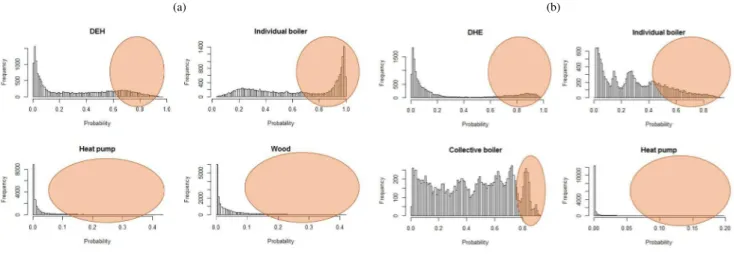
In this section, we propose to analyze the barriers to choosing a particular RSHS. More precisely, we attempt to determine the household and dwelling characteristics for which the considered choice alternative has the highest probability of being chosen. The econometric model for choice of RSHS gives us the estimated probability by year and household. The distribution of probability by choice for 2006 is given in Figure 3 (individual houses and apartments) and for 2013 in Figure 4 (all dwellings). For each choice alternative we try to identify the group of households with the highest probability (orange area in the Figures 3–4).
Figure 3: Distribution of estimated probability for individual houses (a) and apartments (b) in 2006
(a) (b)
Figure 4: Distribution of estimated probability for dwellings in 2013
We observe that the probability of using a heat pump or wood heating in 2006 is very low. The probability of using a heat pump is a maximum of 0.48 and 0.2 in houses and apartments respectively. For many dwellings the probability is close to 0. The same observation applies to wood heating. In contrast, the probability of using a boiler or DEH comes close to 1 for some dwellings. This means that dwelling and household characteristics strongly determine the RSHS for these households. In the case of apartments, we clearly observe several distributions for boilers: individual boilers seem to divide into 5 groups of household, while in the case of collective boilers we observe 9 groups, 7–8 of which seem to comprise the same number of households.
Looking at 2013, we observe a significant change in probability distribution. The probability of having a heat pump or wood RSHS comes close to 0.6. For many dwellings, the probability of having a collective boiler is close to 0. In the case of DEH and individual boilers, the probabilities are still high, but lower than in 2006. We also observe the small number of households whose probabilities are close to 0 in comparison with 2006.
7.1. Global results
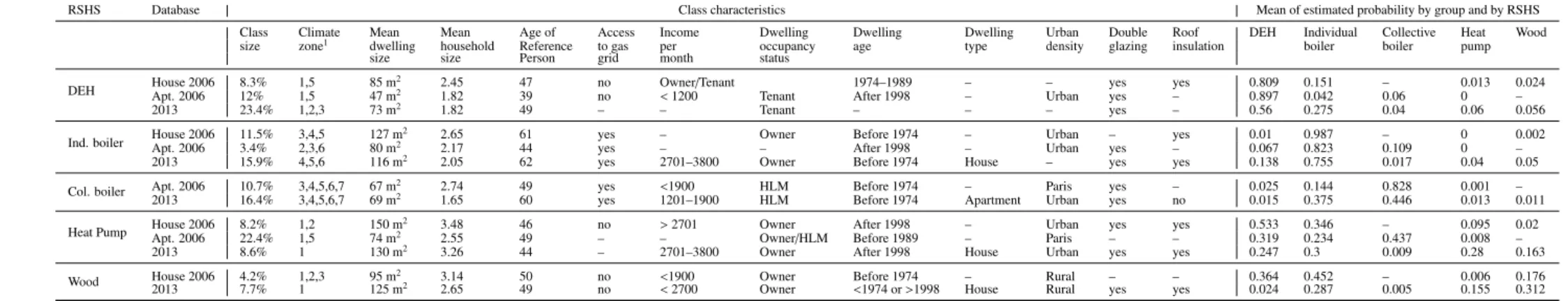
The results of clustering are given in radar charts Figure 5 showing the mean values of characteristics for each group of household in 2006 and 2013. For example, the mean dwelling size for the heat pump group in 2013 is 129 m2which is double the mean dwelling size for the collective boiler group.
Figure 5: Cluster results for individual houses in 2006 (a), for apartments in 2006 (b) and for all dwellings in 2013 (c)
(a) (b) (c)
The detailed results of clustering are given in Appendix A Table A.6. In 2006, the mean probability of having a boiler or DEH by focus group is high compared to the mean probability of the heat pump and wood group: 0.828 for collective boilers in apartments and 0.987 for individual houses. If we consider the number of households with strong constraints, at 0.8 mean probability by cluster, we can conclude that 21% of households living in houses and 36% living in apartments had no choice in 200620. The situation had improved by 2013: only the individual boiler group has a strong constraint, with a mean probability equal to 0.75. If we look at the dwelling occupation status, we note that the group for heat pumps, individual boilers and wood heating is composed of owners. In contrast, the highest probabilities of having a collective boiler concern social tenants in HLMs and other tenants for DEH. The results are the same for both years.
The mean dwelling size in the DEH focused group is the lowest compared to other groups: 85 m2 for the DEH group against 95 m2(wood), 127 m2(individual boiler) and 150 m2(heat pump). In 2013 the mean dwelling size for DEH and collective boiler groups are close to 70 m2, whereas the mean dwelling size for other RSHSs is around 120 m2. The heat pump group has the largest household size: 3.47 people in 2006 (houses) and 3.259 in 2013, followed by individual boilers and wood heating. In 2006, the collective boiler group has the highest mean household size (2.55) in apartments, whereas in 2013 it has the lowest (1.65). The age of reference person for heat pumps, DEH and wood is similar in all models. High income characterizes the heat pump group in 2006 (houses) and 2013. In 2013, households in the individual boiler group also have the high level of income. Households in the boiler groups (both individual and collective) live in dwellings built before the first thermal regulation (1974).
7.2. Direct electric heating
The group weight for DEH is 8.3% in 2006 (houses) and 23.4% in 2013. The mean probability is very high in groups for 2006: 0.809 for houses and 0.897 for apartments. It is clear that for 20.3% of households, dwelling and household characteristics strongly determine the presence of DEH. The mean probability of opting for another RSHS is between 0 and 0.15. These barriers have been overcome in 2013. The mean probability of having DEH is 0.56, but the group weight is 23.4%. In 2006, DEH is widespread in the Mediterranean and semi-continental climates, whereas in 2013 it also concerns a significant number of households in oceanic and middle oceanic climate zones. The mean size of dwelling and the age of reference person changed little between 2006 and 2013. However, the mean size of household decreased from 2.45 (houses) and 1.82 (apartments) people per household in 2006 to 1.82 for all dwellings in 2013. This is in line with general statistics: household size on average dropped from 2.3 in 2006 to 2.16 in 2013. Household groups are not characterized by income (except apartments in 2006) or urban density (except apartments). Access to the gas grid, age of dwelling, income and urban density do not determine which households prefer direct electric heating in 2013.
7.3. Individual boiler
This groups weight increases from 3.4% in 2006 to 15.9% in 2013, with households residing in all climate zones except for the Mediterranean and middle oceanic. We observe a decrease in household size from 2.65 and 2.17 in 2006 to 2.05 in 2013. As for DEH, this is probably due to the general decrease in household size between the two years. The 2013 group is characterized by high income (2701-3800 €/ month). The mean probability of having an individual boiler is 0.987 (houses) and 0.823 (apartments) in 2006, whereas the mean probability of using another RSHS is close to 0. However, in 2013 the mean probability decreases to 0.755 in favor of DEH with a 0.138 mean probability in these group.
7.4. Collective boiler
Collective boilers were preferred by people with average age of 49 in 2006, but the mean reference person’s age was 10 years older in 2013. As in the case of individual boilers, household size decreased between the two years. We do not observe any other changes, except the group weight and mean probability, which was 0.828 in 2006 and rose to 0.446 in 2013, competing with individual boilers, with a mean probability of 0.375 in the same group. Typical households from this group are social tenants on incomes below 1,900 euro per month living in apartments built before 1974 in urban area zone.
7.5. Heat pump
We do not observe any significant differences between the household groups that prefer heat pumps in 2006 and 2013. In both cases, this group is a large young family with a high income, living in a Mediterranean climate zone in a dwelling built after 1998 with a good level of insulation. However, the group for 2013 is more accurate because the mean probability of choosing a heat pump is about 0.22, whereas it was about 0.095 in 2006. In 2006 the mean probabilities for DEH and individual boilers are 0.533 and 0.346 respectively. Looking at 2013, the mean probabilities for other RSHSs are close to that of heat pumps, except for collective boilers (0.0009). We conclude that in 2013 households in this group have no preference between DEH, heat pumps, individual boilers and wood heating.
7.6. Wood heating
Wood heating systems are the preferred choice in the Mediterranean, middle oceanic and oceanic climate zones. The mean dwelling size increased from 95 m2in 2006 to 125 m2in 2013, but household size decreased. In 2006, only low-income households preferred wood. The 2013 group is also characterized by households living in dwellings built before 1974 and after 1998. This may be explained by the spread of wood heating systems from 1% in 2006 to 11.3% in 2013 especially in new buildings. The mean probability of using wood heating is 0.312, followed by individual boilers (mean probability about 0.28) and heat pumps (mean probability about 0.155). The 2013 wood heating group differs from all of the other groups regarding the sum of mean probability, which is 0.783. For the other groups, the sum of probabilities of using all considered RSHSs is close to 1. We can conclude that the households in this group also prefer other RSHSs not mentioned in the study.
8. Conclusion
The aim of this research was to analyze how strong the household situation impacts the likelihood of using different types of RSHS in French dwellings. The quantitative results obtained using econometric methods are consistent with the qualitative knowledge of experts from the energy sector in France. Comparing the results from both years used in the study (2006 and 2013), we identified limited differences in the models. However, we observed that the order of preferences between choice alternatives changed from 2006 to 2013: the probability of choosing wood or a heat pump as a main heating system significantly increased in 2013.
Focusing our study in socio-demographic, dwelling and spatial determinants, we show that in 2006 these charac-teristics strongly determine the type of RSHS for 21% and 36% of households in, respectively, individual houses and apartments. Thus, these households did not seem to have a choice. The situation had improved by 2013, especially for the wood heating focused group, for whom wood heating is the first choice. However this progression is not sufficient, because individual boilers are the second choice for households in all focused groups.
Climate zone seems to be an important determinant of household choice. This suggests that different government incentive policies could be adopted for each climate zone. EM clustering also showed that most focused groups comprise owners, except for collective boilers and DEH in 2013.
We intend to use these results in a model that describes the home renovation market, i.e. insulation and replacement of RSHSs. This type of model could also be used to calibrate energy models or calculate expected energy consumption (Braun, 2010; Nesbakken, 1999). We use the revealed preferences data, which is related to actual choices in real-life situations, but do not give the information on no selected choice alternatives. To improve our study, we will need to conduct the choice experiment on French households. This will give us a stated preferences dataset able to take into account the attributes of all choice alternatives, calculate willingness-to-pay (Goett et al., 2000), and consider the taste heterogeneity of consumers behavior (Islam and Meade, 2013). These two types of data can be combined to make the choice experiment more realistic (Ben-Akiva and Morikawa, 2002).
References
Achtnicht, M. (2011), ‘Do environmental benefits matter? evidence from a choice experiment among house owners in germany’, Ecological
Economics 70(11), 2191–2200.
Achtnicht, M. and Madlener, R. (2014), ‘Factors influencing german house owners’ preferences on energy retrofits’, Energy Policy 68, 254–263. ADEME (2014a), Les chiffres cl´es du bˆatiment 2013, Technical report.
URL: http://www.presse.ademe.fr/2014/04/les-chiffres-cles-du-batiment-2013.html ADEME (2014b), ‘Mener une r´enovation ´energ´etique en copropri´et´e’, Agir! .
Ameli, N. and Brandt, N. (2014), Determinants of households’ investment in energy efficiency and renewables, OECD economics department working papers, Organisation for Economic Co-operation and Development, Paris.
Banfi, S., Farsi, M., Filippini, M. and Jakob, M. (2008), ‘Willingness to pay for energy-saving measures in residential buildings’, Energy Economics 30(2), 503–516.
Ben-Akiva, M. and Morikawa, T. (2002), ‘Comparing ridership attraction of rail and bus’, Transport Policy 9(2), 107–116.
Braun, F. G. (2010), ‘Determinants of households space heating type: A discrete choice analysis for german households’, Energy Policy 38(10), 5493–5503.
CEREN (2011), Secteur r´esidentiel: suivi du parc et des consommation d’´energie et ´evolution 1973-2010, Technical report.
Couture, S., Garcia, S. and Reynaud, A. (2012), ‘Household energy choices and fuelwood consumption: An econometric approach using french data’, Energy Economics 34(6), 1972–1981.
Dempster, A. P., Laird, N. M. and Rubin, D. B. (1977), ‘Maximum likelihood from incomplete data via the EM algorithm’, Journal of the Royal
Statistical Society B 39(1), 1–38.
Dubin, J. A. and McFadden, D. L. (1984), ‘An econometric analysis of residential electric appliance holdings and consumption’, Econometrica 52(2), 345.
Fraley, C., Raftery, A. E., Murphy, T. B. and Scrucca, L. (2012), mclust Version 4 for R: Normal Mixture Modeling for Model-Based Clustering,
Classification, and Density Estimation.
Goett, A. A., Hudson, K. and Train, K. E. (2000), ‘Customers’ choice among retail energy suppliers: The willingness-to-pay for service attributes’,
The Energy Journal 21(4). INSEE (2006), ‘Enquˆete logement’.
URL: http://www.cmh.ens.fr/greco/enquetes/XML/lil-0410.xml
Islam, T. and Meade, N. (2013), ‘The impact of attribute preferences on adoption timing: The case of photo-voltaic (PV) solar cells for household electricity generation’, Energy Policy 55, 521–530.
Laurent, M.-H., Allibe, B. and Osso, D. (2011), ‘Energy efficiency for all! how an innovative conditional subsidy on refurbishment could lead to enhanced access to efficient technologies’, ECEEE 2011 Summer Study .
Laurent, M.-H., Osso, D. and Cayre, E. (2007), ‘Energy savings and costs of energy efficiency measures: a gap from policy to reality?’, ECEEE
2007 Summer Study.
Le Cadre, H., Bouhtou, M. and Tuffin, B. (2009), ‘Consumers’ preference modeling to price bundle offers in the telecommunications industry: a game with competition among operators’, NETNOMICS: Economic Research and Electronic Networking 10(2), 171–208.
Liao, H.-C. and Chang, T.-F. (2002), ‘Space-heating and water-heating energy demands of the aged in the US’, Energy Economics 24(3), 267–284. Mansur, E. T., Mendelsohn, R. and Morrison, W. (2008), ‘Climate change adaptation: A study of fuel choice and consumption in the US energy
sector’, Journal of Environmental Economics and Management 55(2), 175–193.
McFadden, D. (1974), ‘The measurement of urban travel demand’, Journal of Public Economics 3(4), 303–328. McFadden, D. and Domencich, T. (1975), Urban Travel Demand: a Behavioral Analysis.
Michelsen, C. C. and Madlener, R. (2012), ‘Homeowners’ preferences for adopting innovative residential heating systems: A discrete choice analysis for germany’, Energy Economics 34(5), 1271–1283.
Minist`ere de l’´ecologie, du d´eveloppement durable et de l’´energie (2014), ‘P´egase’. URL: http://www.statistiques.developpement-durable.gouv.fr/donnees-ligne/r/pegase.html
Nesbakken, R. (1999), ‘Price sensitivity of residential energy consumption in norway’, Energy economics 21(6), 493–515. Rahut, D. B., Das, S., De Groote, H. and Behera, B. (2014), ‘Determinants of household energy use in bhutan’, Energy 69, 661–672.
Ricci, O. and B´erang`ere, L. (2014), Measuring fuel poverty in france: Which households are the most vulnerable?, EcoMod2014 6923, EcoMod. Rouvinen, S. and Matero, J. (2013), ‘Stated preferences of finnish private homeowners for residential heating systems: A discrete choice
Scasny, M. and Urban, J. (2009), Household behaviour and environmental policy: Residential energy efficiency, OECD, Paris. Schwarz, G. (1978), ‘Estimating the dimension of a model’, The Annals of Statistics 6(2), 461–464.
Thurstone, L. L. (1927), ‘A law of comparative judgment.’, Psychological Review 34(4), 273–286.
Vaage, K. (2000), ‘Heating technology and energy use: a discrete/continuous choice approach to norwegian household energy demand’, Energy
Appendix A. Results of EM clustering
Table A.6: Results of EM clustering
RSHS Database Class characteristics Mean of estimated probability by group and by RSHS
Class Climate Mean Mean Age of Access Income Dwelling Dwelling Dwelling Urban Double Roof DEH Individual Collective Heat Wood
size zone1 dwelling household Reference to gas per occupancy age type density glazing insulation boiler boiler pump
size size Person grid month status
DEH House 2006 8.3% 1,5 85 m
2 2.45 47 no Owner/Tenant 1974–1989 – – yes yes 0.809 0.151 – 0.013 0.024
Apt. 2006 12% 1,5 47 m2 1.82 39 no <1200 Tenant After 1998 – Urban yes – 0.897 0.042 0.06 0 –
2013 23.4% 1,2,3 73 m2 1.82 49 – – Tenant – – – yes – 0.56 0.275 0.04 0.06 0.056
Ind. boiler House 2006 11.5% 3,4,5 127 m
2 2.65 61 yes – Owner Before 1974 – Urban – yes 0.01 0.987 – 0 0.002
Apt. 2006 3.4% 2,3,6 80 m2 2.17 44 yes – – After 1998 – Urban yes – 0.067 0.823 0.109 0 –
2013 15.9% 4,5,6 116 m2 2.05 62 yes 2701–3800 Owner Before 1974 House – yes yes 0.138 0.755 0.017 0.04 0.05
Col. boiler Apt. 2006 10.7% 3,4,5,6,7 67 m2 2.74 49 yes <1900 HLM Before 1974 – Paris yes – 0.025 0.144 0.828 0.001 –
2013 16.4% 3,4,5,6,7 69 m2 1.65 60 yes 1201–1900 HLM Before 1974 Apartment Urban yes no 0.015 0.375 0.446 0.013 0.011
Heat Pump House 2006 8.2% 1,2 150 m
2 3.48 46 no >2701 Owner After 1998 – Urban yes yes 0.533 0.346 – 0.095 0.02
Apt. 2006 22.4% 1,5 74 m2 2.55 49 – – Owner/HLM Before 1989 – Paris – – 0.319 0.234 0.437 0.008 –
2013 8.6% 1 130 m2 3.26 44 – 2701–3800 Owner After 1998 House Urban yes yes 0.247 0.3 0.009 0.28 0.163
Wood House 2006 4.2% 1,2,3 95 m2 3.14 50 no <1900 Owner Before 1974 – Rural – – 0.364 0.452 – 0.006 0.176
2013 7.7% 1 125 m2 2.65 49 no <2700 Owner <1974 or >1998 House Rural yes yes 0.024 0.287 0.005 0.155 0.312
1Mediterranean (1), middle oceanic (2), oceanic (3), fresh oceanic (4), modified oceanic (5), semi-continental (6), mountain (7).