HAL Id: hal-00318347
https://hal.archives-ouvertes.fr/hal-00318347
Submitted on 30 Jul 2007
HAL is a multi-disciplinary open access
archive for the deposit and dissemination of
sci-entific research documents, whether they are
pub-lished or not. The documents may come from
teaching and research institutions in France or
abroad, or from public or private research centers.
L’archive ouverte pluridisciplinaire HAL, est
destinée au dépôt et à la diffusion de documents
scientifiques de niveau recherche, publiés ou non,
émanant des établissements d’enseignement et de
recherche français ou étrangers, des laboratoires
publics ou privés.
an 8000-year precipitation reconstruction from tree rings
in the southwestern USA
Jianmin Jiang, Xiangqian Gu, Jianhua Ju
To cite this version:
Jianmin Jiang, Xiangqian Gu, Jianhua Ju. Significant changes in subseries means and variances in an
8000-year precipitation reconstruction from tree rings in the southwestern USA. Annales Geophysicae,
European Geosciences Union, 2007, 25 (7), pp.1519-1530. �hal-00318347�
www.ann-geophys.net/25/1519/2007/ © European Geosciences Union 2007
Annales
Geophysicae
Significant changes in subseries means and variances in an
8000-year precipitation reconstruction from tree rings in the
southwestern USA
Jianmin Jiang1,2,3, Xiangqian Gu4, and Jianhua Ju1
1Training Center of China Meteorological Administration, Beijing, 100081, China
2Joint Institute of Marine and Atmospheric Research (JIMAR), University of Hawaii, Honolulu, HI, 96822, USA 3Pacific Fisheries Environmental Laboratory, NOAA/NMFS, Pacific Grove, CA, 93950, USA
4Chinese Academy of Meteorological Sciences, Beijing, 100081, China
Received: 2 October 2006 – Revised: 4 June 2007 – Accepted: 27 June 2007 – Published: 30 July 2007
Abstract. Both algorithms were applied to an 8000-year
long time series of annual precipitation that was recon-structed from tree rings in the southwestern USA. One of the algorithms is the scanning t-test, which detects signif-icant changes in subseries means (the first center moments) on various time scales. Another is the scanning F -test, which detects significant changes in subseries variances (the sec-ond center moments) on multi-time scales. Firstly, the scan-ning t -test identified 22 change points in subseries means and partitioned the series into 23 relatively wet, normal or dry episodes. Secondly, the scanning F -test detected 15 change points in subseries variances and divided 16 phases in com-paratively steady (with smaller variance) or unsteady (with larger variance) features. Thirdly, the 23 wetness-episodes were characterized as the steady or unsteady situations by jointing the results from the scanning F -test into those from the t-test. Fourthly, the 23 episodes were compared to those in the TIC and δ18O records from cored sediments in the deep basin of the Pyramid Lake in Nevada by using a coherency analysis of the t -test between the precipitation reconstruction and the TIC or δ18O series. Fifthly, the 23 episodes were col-laborated with some published papers in related studies. In addition, the 23 episodes were also compared with studies of the global climate change and with documents of climate changes in China during the same periods. As the TIC and
δ18O record series are high resolution with unequal sampling intervals between 3 and 14 years, an algorithm in the scan-ning t-test for dealing with the unequal time intervals was developed in this study.
Keywords. Geomagnetism and paleomagnetism (Time
vari-ations, secular and long term) – Meteorology and atmo-spheric dynamics (Precipitation) – General or miscellaneous (Techniques applicable in three or more fields)
Correspondence to: Jianmin Jiang
(jiangjm93950@yahoo.com)
1 Introduction
Hughes and Graumlich (1996) reported a valuable dendro-climatic study of annual (prior July through current June) precipitation reconstruction for the period from 6000 BC to 1996 AD for the climate division 3 in south-central Nevada, based on the Methuselah Walk tree ring chronology from the White Mountains in California, in southwestern USA (Fig. 1). They emphasized the striking pattern of two multi-decadal droughts in the epoch between 900 AD and 1400 AD and listed eight extreme drought years, in which bidecadally filtered values of the precipitation reconstruction were be-low 17 cm. However, no analysis of statistically significant changes was reported for this series before.
Karl and Riebsame (1984) detected fluctuations in air temperature and precipitation in the USA with the Student
t -test. Yamamoto et al. (1986) modified the t-test into
a ratio of signal-to-noise as criterion to analyze “climatic jump”. Goossen and Berger (1987) defined an abrupt cli-mate change or a climatic discontinuity as an abrupt and per-manent change during the period of record from one aver-age value to another, and employed the Mann-Kendall rank test to recognize the abrupt climatic change. However, they discuss only about the subsample average and search only one change point per calculation in a time series. The IPCC (2001) has a consensus that the climate change includes two contents: changes of subseries means (the first center mo-ments) and changes of subseries variances (the second center moments). Jiang et al. (2001, 2002, 2003) grafted the wavelet technique (Kumar and Foufoula-Georgiou, 1994) onto the Student t-test and the F -test (Cramer, 1946) to develop al-gorithms of scanning t -test and scanning F -test, respectively. The scanning t test detects significant changes in the first mo-ments (subseries means or averages) at each time period on various time scales in a long time series, while the scanning
F -test detects significant changes in subseries variance (the
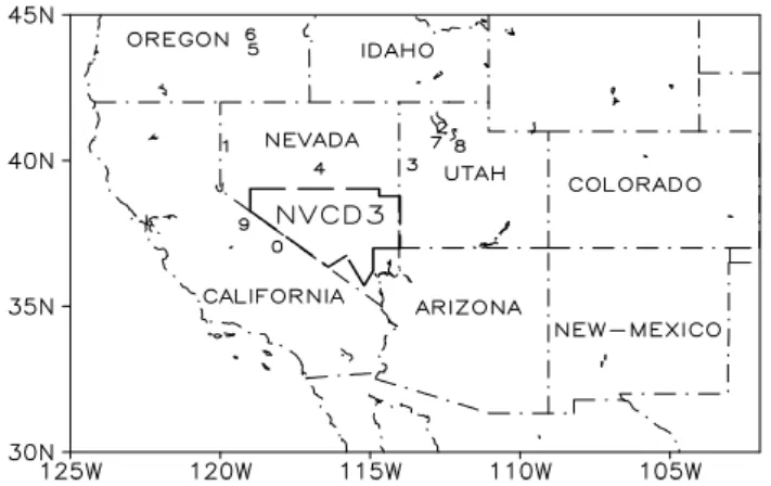
Fig. 1. Locations of the Nevada Climate Division 3 (NVCD3) and
10 numbered sites that are mentioned in Sects. 1 and 6. (The num-bers indicate: 0 – White Mountains, 1 – Pyramid Lake, 2 – Great Salt Lake, 3 – Danger Cave, 4 – Potato Canyon Bog, 5 – Diamond Pond, 6 – Malheur Maar, 7 – Homestead Cave, 8 – Snowbird Bog, 9 – Mono Lake).
in a long time series. The algorithms give thresholds at a given statistical confidence, as well as detect multiple signifi-cant change points on multi-time scales. In order to avoid the argument of how to separate exactly “abrupt change” from “gradual change”, we use “significant change” in both the average and variance instead of “abrupt change” in the av-erage. This may agree more exactly with the statistics. A significant change means that the difference in the subseries statistics between the two adjoining subseries is statistically significant at a given statistical confidence in that statistical test. The statistics include the average or mean (the first ment) and the variance or standard deviation (the second mo-ment) in this study.
This paper attempts to apply both algorithms of the scan-ning t-test (Jiang et al. 2001, 2002) and the scanscan-ning F -test (Jiang et al., 2003) to the unfiltered precipitation reconstruc-tion for the Nevada climate division 3; here the unfiltered precipitation reconstruction represents that has not been fil-tered bidecadally (Hughes and Graumlich, 1996). Firstly, the scanning t-test identifies twenty-two change points, and 23 comparatively climatic wetness-episodes are partitioned in the 8000-year precipitation reconstruction series. Sec-ondly, the scanning F -test detects 15 change points in sub-series variance and divides 16 phases in comparatively steady (with smaller variance) or unsteady (with larger variance) features. Thus, the 23 wetness episodes are characterized as the steady or unsteady traits by joining the results from the scanning F -test into those from the t-test. Thirdly, to verify the significant changes in subseries averages in the unfiltered precipitation reconstruction series, we employ the coherency detection algorithm based on the scanning t-test (Jiang et al., 2002) to the precipitation reconstruction and other two high-resolution time series, the TIC (Total
Inor-ganic Carbon fraction) and δ18O records from cored sedi-ments in the deep basin of the Pyramid Lake (see Fig. 1) in Nevada (Benson et al., 2002). The coherency detection al-gorithm tests synchronously and asynchronously significant changes in the subseries levels between the two time series on multi-time scales. Thirteen change points appear in the precipitation reconstruction which are close to those in the TIC or δ18O series within 150 years of difference and cov-ering the overlapping years by more than 2/3 of the episode duration. Finally, we confirm the 23 wetness-episodes with previously published research into the climatic change peri-ods in the western USA, and find that 22 of the 23 episodes coincide with the previously published results. In addition, the 23 episodes are also compared with studies of climate changes in the eastern China, as well as of global changes. As known, eastern China and western USA are located on the western and eastern coasts of the Northern Pacific, re-spectively, and China is located in the upstream, while the USA are located in the down-stream of the westerlies in the general atmospheric circulation. They are all influenced by the ENSO, and PDO and other factors but with different after effects.
The motives of this study are to examine the practicality of the algorithms, the reliability of the precipitation reconstruc-tion data and to discuss the possible associareconstruc-tions of climate changes in the western USA with the global changes and cli-mate changes in China during the last 8000 years.
2 Methodology
2.1 Two contents of climate change
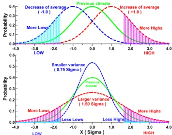
Figure 2 illustrates two aspects of climate change, which were proposed in the IPCC (2001). Suppose a meteorolog-ical element in the normal distribution, when the subseries means (the first moments) move to higher value, the prob-ability of extreme high events (climate disasters) increases, while the probability of extreme low events (opposite climate disasters) decreases, otherwise vice versa (upper panel). On the other hand, when the subseries variances (the second mo-ments) become larger, the probabilities of both sides of the extreme events (climate disasters) increases, and otherwise vice versa (lower panel). In this study, we attempt to in-troduce and apply algorithms for detecting both aspects of significant climate changes.
2.2 The scanning t-test and coherency detection
In the scanning t-test, the statistic t (n, j ) is defined to mea-sure differences of subsample averages between every two adjoining subseries with equal subsample size (n) as follows (Jiang et al., 2002):
t (n, j ) = (xj 2−xj 1) · n1/2·(sj 22 +s
2
j 1)
where xj 1= 1 n j −1 X i=j −n x(i), xj 2= 1 n j +n−1 X i=j x(i); s2j 1= 1 n − 1 j −1 X i=j −n (x(i) − xj 1)2; s2j 2= 1 n − 1 j +n−1 X i=j (x(i) − xj 2)2,
where the subsample size n may vary as n=2, 3,. . . ,<N/2, or may be selected at suitable intervals. The j=n+1, n+2,. . . ,
N–n+1 is the reference time point, at which a significant
change point is to be tested on the time scale n in the time-series with total records N .
For those series with unequal sampling intervals, we let
j denote the order of records in time sequence, while Y (j )
indicates the corresponding year at the j -th record in the chronology. The sample number is taken as {(j–1)–(j–n)} and
{(j+n–1)–j}, respectively, while the time scale (subseries
du-ration) is controlled by letting {Y(j–1)-Y(j–n)} or {Y(j+n–1)–
Y(j)} equal to or less than the given scale. In this work, the
sample size (number) n is less than the time scale.
Since the series examined in this paper are somewhat auto-correlated, for example, in the precipitation reconstruction the lag-1 autocorrelation coefficients vary between −0.29 and +0.26 in pooled subsamples of length 2n. The Table-Look-Up Test (Von Storch and Zwiers, 1999) is adopted to correct the significance criterion of the statistic t (n, j ) ac-cording to the lag-1 autocoefficients of the pooled subsample and the subsample size n. Criterion t005for the correction of
the dependence is usually selected to determine significant changes on time scales longer than 30 years. For shorter sub-sample sizes, the critical values are usually overly restrictive. Since the significance level varies with n and j , to make values comparable, the test statistic is normalized as:
tr(n, j ) = t (n, j )/t0.05, (2)
so that a significant change is at the 95% confidence level when |tr(n, j)|>1.0, with tr(n, j )<–1.0 denoting a significant
decrease, and tr(n, j )>1.0 indicating a significant increase
in the time series.
Finally, a coherency index of significant changes between the two series u and v is defined as the statistic trc(n, j ): trc(n, j )=sign[tru(n, j )·trv(n, j )]{|tru(n, j )·trv(n, j )|}1/2.(3)
Usually, a center (local maximum) of trc(n, j )>1.0 with both |tru(n, j)| and |trv(n, j)| >1.0 represents a pair of significant
changes in the same direction (in-phase), while the center (local minimum) of trc(n, j )<–1.0 denotes a pair of
signifi-cant changes in the opposite direction (anti-phased).
-4.0 -3.0 -2.0 -1.0 0.0 1.0 2.0 3.0 4.0 0.0 0.1 0.2 0.3 0.4 Pr o b a b il it y -4.0 -3.0 -2.0 -1.0 0.0 1.0 2.0 3.0 4.0 X ( Sigma ) 0.0 0.1 0.2 0.3 0.4 0.5 0.6 Pr o b a b il it y Decrease of average ( -1.0 ) Previous climate More Lows LOW Smaller variance ( 0.75 Sigma ) Previous climate
Less Lows Less Highs
Increase of average ( +1.0 ) More Highs HIGH Larger variance ( 1.50 Sigma ) More Lows
Fig. 2. Illustration of two contents in climate changes.
2.3 The scanning F-test
Similarly, in order to detect significant changes in subseries variances (the second centre moments), the index Fr(n, j ) of
the scanning F -test is defined as:
Fr(n, j ) = −(Sj 12 /Sj 22)/Fα, f orSj 2< Sj 1, 0, f orSj 2=Sj 1orSj 1=0, Sj 2=0 (Sj 22/Sj 12 )/Fα, f orSj 2> Sj 1 , (4)
where the subsample standard deviations Sj 1and Sj 2are
cal-culated in the same way as in (1), and similarly n=2, 3, ...,
<N/2, j=n+1, n+2, ..., N-1. Fαis a threshold value on the
ef-fective degree of freedom after the correction of dependence and in a normalized distribution for the time series. A lo-cal minimum in Fr(n, j )<–1.0 denotes a significant change
towards a smaller variance, i.e. the records become much steadier, whereas a local maximum in Fr(n, j )>1.0 indicates
a significant change towards a larger variance, i.e. the records become much unsteadier. In this algorithm, the subseries variance measures deviations from the subseries mean.
The estimation of the effective degree of freedom for the correction of the dependence is taken as (Hammersley, 1946):
Ef (n) = f (n) · [Xk
τ =0r
2(τ )]−1, r(k) → 0 (5)
where f (n) is the degree of freedom listed in the F form.
3 Data sources
Three time series: the unfiltered precipitation reconstruction, the TIC and δ18O records are used in this work. The un-filtered precipitation reconstruction series was downloaded from the website http://www.ngdc.noaa.gov/paleo/drought/
1024 2048 512 256 128 64 -6000 -5000 -4000 -3000 -2000 -1000 0 1000 T im e S c a le ( y e a rs) -2 -1.5 -1 -0.5 0 0.5 1 1.5 2 -6000 -5000 -4000 -3000 -2000 -1000 0 1000 2000 Years (A.D.) -0.4 -0.2 0 0.2 0.4 (a) (b)
Fig. 3. (a) Contours of the normalized scanning t-test for the
pre-cipitation reconstruction series at confidence level 95%. Contour interval is 0.25 but the zero-contour is hidden. Solid lines denote positive values, dashed lines negative values. (b) Change points and episode averages (solid line) from panel (a), 101-year Gaussian fil-tering of the precipitation reconstruction (dashed line), the average over the entire time series is zero after standardization.
(Hughes and Graumlich, 2000). The series contains a recon-structed annual (prior July-current June) precipitation (in cm) for the Nevada Climate Division 3 (see the NVCD3 in Fig. 1), including a total of 7997 years from 6000 BC to 1996 AD (re-ferred to as the precipitation reconstruction hereafter). It was reconstructed by using the whitened Methuselah Walk tree ring chronology from the White Mountains of California; the location is shown as number “0” in Fig. 1. Other numbered sites in Fig. 1 will be mentioned below and in Sect. 6. This tree ring chronology is the longest absolutely dated in a sin-gle species of the bristlecone pine, at almost 9000 years long. It is made up of 285 tree ring samples with a mean length of 748 years, of which about 14 series are present in each year for the whole period after 6000 BC. These tree ring samples were collected by the Laboratory of tree ring Research, Uni-versity of Arizona. In order to remove any growth trend of the trees, they standardized all tree ring samples with either negative exponential or a straight line with a zero or nega-tive slope. The Box-Jenkins model was fitted (ARMA 1, 1), which accounted for only 5.74% of the series variance, and the series was whitened by computing the residuals from this model. The whitened Methuselah Walk chronology was cal-ibrated in regression to annual precipitation observations in the Nevada Climate Division 3 during the period from 1932 to 1979, and then extrapolated to other years. This regres-sion fitted 35% variance of the precipitation observations. Both power spectrum and singular spectrum analyses indi-cate that very little of the variance of this chronology can be represented by trend, or by periodic or quasi-period
compo-nents. More details about the data are described in Hughes and Graumlich (1996).
The TIC and δ18O high-resolution records from cored sed-iments in the deep basin of the Pyramid Lake (see number “1” in Fig. 1) in Nevada were kindly provided by L. Benson at USGS. These data sets were sampled from 2 piston cores of sediments in the center Pyramid Lake in 1997 (referred as PLC97-1) and in 1998 (PLC98-4), separately. The sites of the 2 cores are very close to each other. The PLC97-1 covers the period from 793 BC to 1839 AD and 533 records were read at unequal intervals between 3 and 9 years. Its age control was established by comparing its palemagnetic sec-ular variation (PSV) record with a well-dated western USA archeomagnetic record (Lund, 1996), and the age model ac-curance was considered within 50–100 yr. The PLC98-4 was taken to recover older Holocence-age sediments, which cov-ers the period from 5680 BC to 1480 BC, and 538 records were read in unequal intervals between 4 and 14 years. Ra-diocarbon ages were determined on the TOC (Total Organic Carbon fraction) of this core and probably remained as larger errors. Further descriptions of the TIC and δ18O data sets can be found in Benson et al. (2002).
4 Significant changes in precipitation reconstruction
se-ries
4.1 Results from the scanning t-test
The scanning t -test was computed for time scales (subsam-ple sizes) ranging from 54 to 2896 years following equation (1) and (2) at a 95% confidence level. We calculate the time scales up to 2896 years in consideration mainly of two rea-sons: one is the mathematical capability, and the other reason is that more than 10 tree ring series cover the whole period after 6000 BC. Based on the local maxima and minima of the t -test values, twelve positive (increases in precipitation reconstruction) and ten negative (decreases in precipitation reconstruction) centers were picked up, i.e. 22 significant change points were discovered by our computing program (Fig. 3a).
For example, the first significant change point towards an increase in precipitation reconstruction is detected with a positive center of the contours around 5865 BC on a 128-year time scale. It was followed by a negative center, a decrease in precipitation, in about 5706 BC on a little shorter time scale. Then the precipitation reconstruction increased once more around 5339 BC on a 91-year scale and in 4606 BC on a 304-year scale. The second decrease point is in 4313 BC on time scale of 362 years. Then two significant increases occurred in 3770 BC and 3205 BC around time scales of 724 years. This may reveal a step-wise approximation to what appears to have been a longer period of increasing precipita-tion in the series. A few local centers of the contours on time scales longer than 750 years, such as in around 3400 BC,
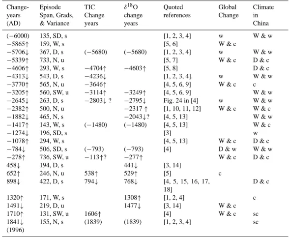
Table 1. Change points and Wet /Normal/Dry episodes in the Precipitation reconstruction series, and sources of collaborative evidence (TIC,
δ18O, paleoclimate references) for each episode.
Change-years (AD) Episode Span, Grads, & Variance TIC Change years δ18O change years Quoted references Global Change Climate in China (−6000) 135, SD, s [1, 2, 3, 4] w W & w −5865↑ 159, W, s [5, 6] W & c −5706↓ 367, D, s (−5680) (−5680) [1, 2, 3, 4] w W & w −5339↑ 733, N, u [5, 7] W & c D & c −4606↑ 293, W, s −4704↑ −4603↑ [5, 8] D & c −4313↓ 543, D, s −4236↓ [1, 2, 3, 4]. w W & w −3770↑ 565, N, u −3646↑ [4, 5, 6, 9] W & c c −3205↑ 560, SW, u −3114↑ −3249↑ [4, 5, 6, 9] W & w −2645↓ 263, D, s −2803↓ ? −2795↓ Fig. 24 in [4] w W & w −2382↑ 500, N, u −2317 ↑ [1, 10, 11, 12] W & c W & c −1882↓ 465, N, s −2043↓? [4, 5, 13] W & w −1417↑ 143, W, s (−1480) (−1480) [4, 5, 13] W & c −1274↓ 196, SD, s [3] w −1078↑ 294, W, s [4, 5, 13] W & c D & c −784↓ 506, SD, s (−793) (−793) [4] D & w W & w −278↑ 736, SW, u −113↑? −277↑ W & c D & c 458↓ 194, D, s 441↓ [3, 14] 652↑ 246, N, u 538↑ 529↑ [5] c 898↓ 422, D, s 794↓ 768↓ [4, 5, 15, 16, 17, 18] D & c 1320↑ 171, W, s 1308↑ [1, 2, 4] c 1491↓ 219, D, u 1477↓ [3, 14] W & c 1710↑ 131, SW, u 1606↑ [4] W & c sc 1841↓ 155, N, s (1839) (1839) [1, 2, 3, 4] sc (1996)
*Notes: A minus sign denotes years in BC.
↑indicates a change to wet; ↓ change to dry.
Numbers in the second column denote the span from a given change year to the next. SD: Severely Dry; D: Dry; N: Normal; W: Wet; SW: Severely Wet.
s: Steady; u: Unsteady; w: Warm; c: Cold; sc: Severe cold. ( ): The beginning and ending years of the data.
[1] Benson et al. (2002), [2] Feng and Epstein (1994); [3] Hughes and Graumlich (1996); [4] Wigand (1987); [5] Madsen et al. (2001); [6] Murchison and Mulvey (2000); [7] Rhode and Madsen (1998); [8] Madsen (1985); [9] Madsen and Currey (1979); [10] Hattori (1982); [11] Long and Rippeteau (1974); [12] Stine (1990); [13] Murchison (1989); [14] Hughes and Funkhouser (1998); [15] Harper and Alder (1970);
[16] Harper and Alder (1972); [17] Madsen and Simms (1998); [18] Stine (1994)
possibly result from those tree ring series covering the whole period after 6000 BC. Each change point is shown in Fig. 3b and listed in Table 1.
These 22 change points partition the unfiltered precip-itation reconstruction series into 23 episodes of relatively stable mean precipitation, which are estimated from the episode averages of precipitation reconstruction for that episode (Fig. 3b). The episode averages can be sorted into 5 grades of climate-scale wetness: Severely Dry (SD) <19.1 cm; 19.1<Dry (D)<19.6 cm; 19.6<Normal (N)<19.9 cm; 19.9<Wet (W)<20.3 cm and Severely Wet (SW)>20.3 cm, respectively (Table 1). It suggests that this region is in an arid-semiarid climatic category. Compared to
Hughes and Graumlich (1996), who analyzed the bidecadally filtered precipitation reconstruction series, the eight years la-beled as extreme droughts in their Table 2 are ranked as Se-vere Dry or Dry episodes in our analysis. The striking multi-decadal droughts between 900 AD and 1400 AD in Hughes and Graumlich (1996) are very similar to the Dry episode 898–1319 AD in our partition.
The 23 episodes span between 131 years (the SW-episode in 1710 AD–1840 AD) and 736 years (the SW-episode in 278 BC–457 AD). The average duration is 348 years (Ta-ble 1). This suggests that the precipitation changes on multi-centennial time scales in this analysis. This result might be technologically reasonable in the dentrochronology, because
-6000 -5000 -4000 -3000 -2000 -1000 0 1000 T im e Sc a le ( Y r. ) -1.5 -1.0 -0.5 0.0 0.5 1.0 64 128 256 512 1024 2048
Fig. 4. (a) Contours of the index of scanning F -test on precipitation
reconstruction series at 95% significance level. Contour interval is 0.25 but the zero-contour hidden. Solid lines denote positive values, dashed lines negative values. (b) change points and period averages of standard deviation (red line) from panel (a), change points and episode averages of precipitation (blue line) same as in Fig. 3b, and unfiltered precipitation reconstruction values (green dashed line).
the longest episode duration of 736 years is shorter than the average length of 748 years of the tree ring samples. Among the 5 grads, the SD and D-grads take over a total of 2845 years, around 35.6% of the total 7997 years, the N-grad oc-cupies the sum of 2664 years, 33.3%, and the W-SW grads cover 2487 years in sum, i.e. 31.1% of the total 7997 years. 4.2 Results from the scanning F-test
The scanning F -test (Eq. 4) of the precipitation reconstruc-tion series was calculated on the same time scales as in Fig. 3. Figure 4a shows many frequent variations on short time scales. On time scales longer than 128 years, how-ever, seven positive (increases of subseries variances) and eight negative (decreases of subseries variances) significant changes were detected, with local maxima and minima in the contours (Fig. 4a). The change years are usually different from those in the first moment (subseries means). Gener-ally, a smaller standard deviation is featured, which means a steadier climate, in the latter period after 2000 BC, than that in the earlier period. We may characterize each episode as a steady or unsteady feature by combining these results with those episodes that were partitioned in Sect. 4.1. For instance, the episode 5339 BC–4607 BC is featured as un-steady (symbolized as “u” in the second column of Table 1), because a large standard deviations (Fig. 4b) corresponds to that. The feature steady (symbolized as “s” in the second column of Table 1) for the episodes 4606 BC–4314 BC and 4313 BC–3771 BC follow, because smaller standard devia-tion (Fig. 4b) coincides with them comparatively, and so on.
Statistically from Table 1, there are 8 steady in proportion to 1 unsteady for a total of 9 episodes in the SD-D grads, 5 steady in ratio to 3 unsteady for a total of 8 episodes in the W-SW grads, while 2 steady comparing to 4 unsteady of 6 episodes in the N-grad. Why the W-SW grads have a slightly higher ratio of unsteady episodes than those in the SD-D grads, is perhaps partly influenced by the tree growth, which is not perfectly removed in the reconstruction process, because it results in a high mean (increased tree ring growth or width) which is naturally related to a high variance (in-creased growth variance) by factors that are internal to tree growth, not to climate (Cook and Peters, 1997). However, five steady of the eight high-mean episodes W-SW are still dominant. This implies here that the F -test of the precipita-tion reconstrucprecipita-tion can reflect mainly the significant climate-change information.
5 Comparison with sedimentary records
This section presents some approximately synchronous changes in subseries means in the precipitation reconstruc-tion with those in the TIC or δ18O records, which are built from cored sediments of Pyramid Lake, Nevada (Benson et al. 2002). Their coherency analyses of subseries-variance changes are not included, because there are multi-millennial trends in both the TIC and δ18O series, especially in the ear-lier period from 5680 BC to 1480 BC (see Fig. 7). Benson et al. (2002) stated that the lake volume fluctuations, as well as fluctuations of the δ18O or TIC records are not simply lin-early correlated. In general, droughts lead δ18O to increase initially as the lake’s volume decreases, but the steady-state value of δ18O for a long drought period is much smaller than that in a wetter period. During wet episodes, Pyramid Lake receives more inflows from its source, the Truckee River, and thus has higher δ18O values. TIC is expected to paral-lel changes in δ18O for long dry and wet periods.
The coherency of significant changes in the precipitation reconstruction series with those in the TIC series for ear-lier years (Fig. 5e) shows four positive coherency (in-phase), centers around 4700 BC and 4230 BC on a 256-year scale, in 3680 BC on a 2048-year scale, and in 3100 BC on a 512-year scale, respectively, despite the presence of three weak nega-tive coherency centers. Some but not all of the change points in the individual series (Figs. 5a and c) coincide closely. For instance, the TIC change points (centers in Fig. 5a) in 4704 BC, 4236 BC, 3646 BC and 3114 BC are close to those in 4606BC, 4313BC, 3770BC, and 3205BC in the precip-itation reconstruction series (centers in Figs. 3a or 5c), re-spectively, by differences within 150 years. The last weak change around 2803 BC in TIC (Fig. 5a) preceeded that in the precipitation reconstruction series by 158 years, so that the coherency is not obvious; we listed this in Table 1 with a question mark. Two possible explanations for the differences in significant change years between the two series are firstly,
-1.50 -1.25 -1.00 -0.75 -0.50 -0.25 0.00 0.25 0.50 0.75 1.00 1.25 1.50 1.75 T im e S c a le (y e a rs) -5000 -4000 -3000 -2000 -500 0 500 1000 1500 (a) (b) (c) (d) (e) (f) 64 128 248 512 1024 64 64 128 128 512 512 248 248 1024 1024
Fig. 5. Contours of the normalized scanning t -test at a 90%
signifi-cance level: (a–b) for the TIC series from Pyramid Lake sediments
(c–d) for the precipitation reconstruction series at same
year/time-scale grids as in panels (a–b); (e–f) the coherency of abrupt changes between panels (a) and (c), (b) and (d), respectively. Contour in-terval is 0.25 but contour zero hidden. Solid lines denote positive values, dashed lines negative values.
chronological errors, especially in the sediment records com-paring to the tree ring reconstruction, and secondly, different locations where the data were collected from.
For later years, Fig. 5f displays 5 positive coherency cen-ters at 200 BC, 190 AD, 330 AD, 640 AD and 870 AD (com-paratively weaker) on scales longer than 300 years, except for some weak, negative coherency centers on time scales shorter than 300 years, i.e. significant changes in the TIC se-ries are mainly in-phase with those in the precipitation recon-struction series on time scales longer than 300 years, while anti-phased are on scales shorter than 300 years. This re-sult agrees with Benson et al. (2002), as mentioned above in the first paragraph of this section. The TIC change points (Fig. 5b) in 113 BC, 538 AD, 794 AD and 1606 AD are ap-proximately close to those in the precipitation reconstruction at 278 BC, 652 AD, 898 AD and 1710 AD, respectively (Ta-ble 1 or Fig. 7). As the TIC change year 113 BC occurred 165 years later than the change point in 278 BC in the pre-cipitation reconstruction, we list it in Table 1 with a question mark. The TIC change year 214 AD, which preceded the change point 458 AD in the precipitation reconstruction by 244 years, is not listed in Table 1.
Similarly, Fig. 6c demonstrates the coherency of signif-icant changes between the δ18O (Fig. 6a) and the precip-itation reconstruction (see Fig. 5c) for the earlier period, and unmasks five weak, positive coherency centers around 4620 BC–3710 BC, 3300 BC, 2750 BC and 2240 BC, respec-tively. The coherency here is weaker than that between the TIC and the precipitation reconstruction series (Fig. 5e), be-cause changes in the δ18O series itself are weaker. However, the change points detected in the δ18O series in 4603 BC– 3249 BC, 2795 BC and 2317 BC (Fig. 6a), are comparable to those in the precipitation reconstruction series (Table 1 or
-500 0 500 1000 1500 T im e Sca le ( y e a rs) -5000 -4000 -3000 -2000 64 64 1024 1024 512 512 248 248 128 128 (a) (b) (c) (d)
Fig. 6. (a–b) as same as in Figs. 5a–b but for the δ18O series; (c–d) as same as in Figs. 5e–f but for coherency between the δ18O and the precipitation reconstruction series.
Fig. 7). In addition, the δ18O change point in 2043 BC was 161 years earlier than that in the precipitation reconstruction (Table 1 or Fig. 7), the coherency index (Fig. 6c) is negative in sign, so we list it with a question mark in Table 1. Because the time scale of the positive coherency center in 3710 BC (Fig. 6c) is too long to identify changes in multi-centenary time scales in the δ18O series, no corresponding change year is listed in Table 1.
For the later period, in Fig. 6d, most coherency centers are positive (in-phased changes) on longer time scales, except for a negative coherency center during 300–500 AD, while more negative centers (anti-phased changes) than positive ones ap-pear on shorter time scales. This feature basically coincides with the description by Benson et al. (2002), as quoted in the first paragraph of this section. Though the coherency is obviously weaker than that in Fig. 5f, there are six in-phased changes around 200 BC, 230 AD, 640 AD, 890 AD, 1320 AD and 1500 AD on scales longer than 100 years. The abrupt changes 277 BC, 441 AD, 529 AD, 768 AD, 1308 AD and 1477 AD for the δ18O series may correspond to those in the precipitation reconstruction series (Table 1 and Fig. 7).
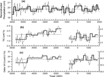
Further comparisons, by calculating the episode averages for each series based on the detected change points for that series and by using a 101-year Gaussian filter to low-pass filter each series, are illustrated in Fig. 7. An obvious differ-ence is that the millennial-scale trends in both the TIC and
δ18O series in the earlier period, from 5680 BC to 1480 BC, are much more apparent than that in the precipitation recon-struction. As mentioned in Sect. 3, the precipitation series is reconstructed from tree rings with an average length shorter than 750 years and with a standardization of every tree ring sample, which may preclude any millennial-scale trend in the precipitation reconstruction series.
Even so, there are common features in the episode av-erages and smoothed data of the three series. In the mid-dle Holocene, the Dry episode in 5706–5340 BC, the Wet episode in 4606–4314 BC, the Severely Wet episode in 3205–2646 BC and the Dry episode in 2645–2383 BC iden-tified in the partitioned precipitation reconstruction series (Fig. 7a) have rough equivalents to those in the other two
-6000 -5000 -4000 -3000 -2000 -1000 0 1000 0.5 1.0 1.5 2.0 2.5 T IC ( u n it % ) -6000 -5000 -4000 -3000 -2000 -1000 0 1000 Year (AD) 26 27 28 29 30 D e lt a 1 8 O ( u n it 0 .1 % ) 2.0 2.4 2.8 29.5 30.0 30.5 31.0 (b) (c) (a) -6000 -5000 -4000 -3000 -2000 -1000 0 1000 2000 18 19 20 21 R e c o n s tr u c te d P re c ip it a ti o n ( c m )
Fig. 7. The change points and episode averages (solid line),
101-year Gaussian filter (dashed line) and averages over the entire time series (dotted line) in the three series: (a) same as in Fig. 3b; (b) for the TIC and (c) for the δ18O series from sediment cores in Pyramid Lake.
series (Figs. 7b and c). The Dry episode in 4313–3771 BC and the Normal episode in 3770–3206 BC in the precipita-tion reconstrucprecipita-tion have analogs in the TIC series, while the Normal episode in 2382–1883 BC and 1882–1418 BC ap-proximate those in the δ18O series. Only the Normal episode in 5339–4607 BC is not collaborated by either the TIC or
δ18O series.
During the late Holocene, the Severely Dry episode in 784∼279 BC, the Severely Wet episode in 278 BC–457 AD, the Dry episode in 458–651 AD, the Normal episode in 652– 897 AD and the Dry episode in 898–1320 AD are similar among the three series (Fig. 7). The Wet episode in 1320– 1490 AD and the Dry episode in 1491–1709 AD in the pre-cipitation reconstruction (Fig. 7a) are roughly comparable to those in the δ18O series (Fig. 7c). The Severely Wet episode in 1710–1840 AD in the precipitation reconstruction (Fig. 7a) is similar to that in the TIC series (Fig. 7b).
Interestingly, the period from 1479 to 794 BC, in which the TIC and δ18O series were disconnected between the piston cores PLC98-4 and PLC 97-1, is identified as a period of very strong changes on short time scales in the precipitation reconstruction (Fig. 7a).
6 Verification with related studies
Although the precipitation reconstruction is for the Climate Division 3 in Nevada, the tree ring samples composed of the unfiltered precipitation reconstruction were collected from the White Mountains in California. Moreover, because the significant changes identified in this paper are presented on multi-centennial time scales, climate changes usually oc-curred in a large geographical area, especially during dry
periods. Thus, we can consider the changes in the precipi-tation reconstruction series as an epitome of what happened in the western USA. Given this, we may try to use previously published archaeological reports about that region to further collaborate our partition results.
Some related papers published in the last 30 years have examined climatic fluctuations in precipitation or air-temperature in the western USA based on analyses of sedi-ments, pollen, vegetation and tree rings, besides Hughes and Graumlich (1996) and Benson et al. (2002). For example, Madsen et al. (2001) analyzed remains of small animals from stratified raptor deposits, together with fossil woodrat mid-den samples, to partition climate epochs in the eastern Great Basin during the late Pleistocene and Holocene. Grayson (2000) interpreted a decrease in small mammal fauna in the Bonneville Basin of north central Utah as evidence of a dry climate during the Middle Holocene. Benson et al. (1997) in-vestigated δ18O and TIC changes in Owens Lake of the Great Basin for the period from 17 000 BP to 4500 BP. Feng and Epstein (1994) studied a hydrogen isotope time series cover-ing the last 8000 years from Bristlecone Pines in the White Mountains of California. Stine (1994) synthesized data from relict tree stumps in Mono Lake and Tenaya Lake in Califor-nia, and in southernmost Patagonia in South America (48◦S– 50◦S), to determine extreme and persistent drought in Cal-ifornia and Patagonia during medieval times. Stine (1990) presented lake-level fluctuations in Mono Lake, California, for the last 4000 years. Wigand (1987) described the changes in vegetation for the last 6200 years at Diamond Pond in the eastern Oregon desert. However, no report of variance changes was found in these research studies, so we discuss only changes in episode means in this section.
For comparison to these studies, we take 1950 as the present year to convert years before present (BP) into calen-dar years (BC/AD). As mentioned above, sediment cores and pollen records have a dating accuracy of about 50–100 years, even more in multi-millennial chronology. The records from cores may also be biased in reflecting the extreme events of climatic droughts or floods, rather than the average con-ditions over multi-centennial periods. These will make the alignment of dates only approximate and for rough, but use-ful, verifications of the climate situations.
The middle Holocene period from 6000 BC to 3300 BC is commonly recognized to be dry and warm in the Great Basin area, which covers most of Nevada and neighboring re-gions of southeastern Oregon, eastern and southeastern Cal-ifornia, and western Utah (Benson et al., 2002; Madsen et al., 2001; Grayson, 2000; Feng and Epstein, 1994; Wigand, 1987). Five of the eight extreme droughts were distinguished around 5970, 5881, 5591, 4058 and 3948 BC, respectively, by Hughes and Graumlich (1996). This epoch also coin-cides with the global first long warm phase during the last ten thousand years, known as the Europe Climatic Opti-mum period (Asakura, 1991). In our analysis (Table 1), the Severely Dry episode in 6000–5866 BC and Dry episodes
in 5706–5340 BC, 4313–3771 BC occurred in this period. Moreover, the above-mentioned five of the eight years of extreme droughts in Hughes and Graumlich (1996) are in-cluded in these three Dry episodes. In China, the climate in this period also featured warm and wet conditions, glaciers retreated in the western mountains while the desert shrunk in Inner-Mongolia. The Lake Daihai (112◦39′E, 40◦30′N), for example, was four times the area of that at present, and the “Painted Pottery Literature” developed in the middle-reaches of the Yellow River in China during this period (Ye and Chen, 1992).
However, there exist comparatively short wet spells dur-ing this long warm phase. For instance, most glaciers on the Earth progressed around 5400 BC (Goodess et al., 1992). Around 5700 BC the Great Salt Lake level had risen up to its normal level at about 1283 m, which was estimated from marsh deposits (Madsen et al., 2001; Murchison and Mulvey, 2000). This may confirm the Wet episode in 5865–5707 BC in our Table 1. There is a good fit to the Normal episode in 5339–4607 BC (Table 1) by Madsen et al. (2001), who quoted that between 5450 BC and 4750 BC (Rhode and Mad-sen, 1998) single-leaf pinyon nut hulls first appeared in the archaeological record from the Danger Cave (see Fig. 1) in the west of the Great Salt Lake Desert, suggesting a wetter climatic environment than earlier. Other reports by Madsen et al. (2001) and Madsen (1985) state that a spell of greater effective moisture is indicated by a pronounced increase in the abundance of pine at the Potato Canyon Bog (see Fig. 1) in central Nevada between 4550 BC and 4050 BC; this agrees with the Wet episode in 4606–4314 BC (Table 1). In China, two comparatively low magnetization-rates were recorded around 5330 BC and 4700 BC in the loess sediments at Baxie (103◦24′E, 36◦42′N) in Gansu province, denoting a rela-tively cold and arid climate (Ye and Chen, 1992). Fang et al. (2004) summarized cold events around 5450 BC, 4750 BC and a cold period from 4450 BC to 4250 BC in China based on a statistical analysis of cold events or periods based on 97 investigation articles published before.
Wigand (1987) classified the phase from 3510 to 1850 BC into the first wet period that heralded the end of the mid-Holocene drought; it is evidenced that sagebrush pollen in-creases in the perennial Diamond Pond (Fig. 1) in the eastern Oregon desert, and that the littoral and aquatic plant macro-fossils and mollusk shells appeared with sudden abundance shortly before 3510 BC at Malheur Maar (Fig. 1) in the east of Oregon. Madsen et al. (2001) stated that between 3350 BC and 2450 BC, there was an increase in artiodactyl fecal pel-lets at Homestead Cave (Fig. 1) in Utah, and quoted a mean lake-level elevation of 1280 m or lower in the Great Salt Lake (Murchison and Mulvey, 2000) and markedly cooler condi-tions after 3350 BC at Snowbird Bog (Fig. 1) in Utah (Mad-sen and Currey, 1979). These suggest a normal or wetter climate, and lend some credence to the Normal episode in 3770–3206 BC and the Wet episode in 3205–2646 BC in our Table 1. Meanwhile, most glaciers on the Earth
devel-oped again between 3500 BC and 2400 BC (Goodess et al., 1992). Fang et al. (2004) identified a cold period from 4050 to 3450 BC and a cold event in 2950 BC in China.
For the Dry episode in 2645–2383 BC in our Table 1, Fig. 24 in Wigand (1987) shows decreases in the juniper pollen percentage and in the ratio of grass to sagebrush pollen, which mark a drier climate during this spell, though an accompanying description was lacking in the text.
Benson et al. (2002) summed up the findings by Long and Rippeteau (1974), Hattori (1982), Wigand and Mehringer (1985), Grayson (1993), Stine (1990), and others, that there was a wet phase from 2300 BC–1700 BC. This is consistent with the Wet episode in 2382 BC–1883 BC in Table 1. Mad-sen et al. (2001) sorted the period from 2450 BC to 1000 BC as cooler with higher water levels in the lakes, of which the Great Salt Lake level peaked up to 1284 m in 1450 BC (Murchison, 1989), and the following period from 1000 BC to 450 BC was regarded as much wetter and cooler. Wigand (1987) found that the period from 2050 BC to 450 BC was very wet with the deepest late-Holocene pond (Diamond pond) around 1750 BC. These descriptions have some corre-spondence with the Normal episode in 1882 BC–1418 BC, the Wet episodes in 1417 BC–1275 BC and 1078 BC– 785 BC in our Table 1, of which the Wet episode in 1078 BC– 785 BC also coincided roughly with the glacier advances in the Northern Hemisphere (Goodess et al., 1992).
Bond et al. (1997) found two cold events around 2350 BC and 850 BC in the North Atlantic by analyzing concentration of lithic grains and petrologic tracers in Holocene sediments of two cores from opposite sides of the North Atlantic. In China, there were cold periods from 2050 BC to 1750 BC, from 1450 BC to 1250 BC and from 950 BC to 750 BC (Fang et al., 2004), in which the Hanshui River had frozen twice in 903 BC and 897 BC, respectively (Zhu, 1979).
The Severely Dry episode of 1274 BC–1079 BC (Table 1) contains the year 1251 BC, one of the eight extreme dry years found by Hughes and Graumlich (1996). No report of cold events was presented for the years between 1200 BC and 1000 BC by either Bond et al. (1997) or by Fang et al. (2004). It was known as an optimal period of a warm and wet envi-ronment in China (Zhu, 1979), and was found that there were elephants in the north of Henan province, south of the Yel-low River in eastern China during the spell from 1300 BC to 1100 BC (Ye and Chen, 1992).
Though the Severely Dry episode in 784 BC–279 BC in Table 1 diverges from the generally wet conditions for this period suggested by Madsen et al. (2001) and Wigand (1987), a brief but significantly drier period after 650 BC is noted, in which it was reflected by less-abundant floating and submerged aquatic plants at Diamond Pond (Wigand, 1987). During this time most glaciers on the Earth receded (Good-ess et al., 1992). In China, the climate returned to a warm phase from 700 BC to 20 AD (Zhu, 1979), but with a relative cold period from 350 to 250 BC (Fang et al., 2004).
The Dry episodes of 458 AD–651 AD and 1491 AD– 1709 AD in Table 1 are also recognizable as dry periods by Hughes and Graumlich (1996), as well as by Hughes and Funkhouser (1998), who showed that there was a greater in-cidence of intense persistent moisture deficits after 400 AD and before 1500 AD in the Great Basin of North America. However, a cold event in 550 AD in the North Atlantic was reported by Bond et al. (1997).
For the Normal episode in 652 AD–897 AD in Table 1, Madsen et al. (2001) give evidence that around 750 AD a kind of fish, at Utah chub, thrived and that hackberry en-docarps were common, which indicates significantly moister conditions in the Homestead Cave vicinity. During this pe-riod most glaciers advanced again on the Earth, and the sum-mer in Europe and Asum-merica was comparatively cold (Good-ess et al., 1992). In China, however, it was relatively warm between 600 AD and 1000 AD, droughts occurred in the middle-reaches of Yellow River and no snow and ice were seen in Xi’an city, the Capital of Shanxi province, for sev-eral winters (Zhu, 1979; Ye and Chen, 1992), but Fang et al. (2004) concluded a cold event around 850 AD.
Previous investigations also appear to be consistent with the Dry episode in 898 AD–1319 AD in Table 1. For ex-ample, Stine (1994) designates the years from 900 AD to 1200 AD as a period of extreme and persistent drought in California, based on analysis of the tree rings at Mono Lake (Fig. 1). Madsen et al. (2001) summarized that between 1250 AD and 1320 AD, widespread droughts caused people to shift to full-time foraging in the Bonneville Basin (Madsen and Simms, 1998), and the period from 950 AD to 1320 AD may have been one of the warmest and driest phases in the Holocene (Harper and Alder, 1970, 1972). Wigand (1987) concluded that around 1250AD and 1450 AD there were two major droughts indicated by increases in greasewood values in Diamond Pond sediments.
Wigand’s drought in 1450 AD is just earlier than the Dry episode in 1491 AD–1709 AD in our Table 1 by less than 50 years, which might be considered as to coincide with each other. The period from 900 AD to 1300 AD is called the Me-dieval Warm Epoch in the global change literature, the sec-ond warm phase during the last ten thousand years (Asakura, 1991). Most glaciers on the Earth retreated during this phase (Goodess et al., 1992). In China, however, the average tem-perature was a little lower than at the present, though under-going shorter fluctuations from warm (600 AD to 1000 AD), to cold (1000 AD to 1200 AD), to warm again (1200 AD to 1300 AD), and to another cold (1301 AD to 1600 AD) (Zhu, 1979), so that Fang et al. (2004) classified the period from 1150 AD to 1850 AD as a cold phase.
There is collaborative evidence for the Severely Wet episode in 1710 AD–1840 AD in Table 1. Wigand (1987) discerned 1650 AD–1800 AD as wet with abundant juniper and grass pollen. Feng and Epstein (1994) concluded that there was a cool climate spell peaking between 1700 AD and 1900 AD. This period corresponds to the Little Ice Age in
Europe, and the glaciers advanced on the Earth (Goodess et al., 1992). Bond et al. (1997) also reported a cold event around 1650 AD in the North Atlantic. China also experi-enced its coldest phase from 1601 AD to 1899 AD during the last 5000 years (Zhu, 1979; Ye and Chen, 1992).
It is easy to understand that the last episode since 1841 AD is in the Normal category (Table 1), because the precipita-tion reconstrucprecipita-tion is based on a regression analysis between the tree ring records and the precipitation observations in the Nevada Climate Division 3 during the same period from 1932 AD to 1979 AD (Hughes and Graumlich, 1996). This episode roughly corresponds to the third warm phase after 1850 AD in the global change during the last ten thousand years (Asakura, 1991). The declining trend (increase dry-ness) in the low-pass filtered curve of the precipitation re-construction (Fig. 7a) for the last 50 years might reflect the global warming in the last century. The warming in China for the last 50 years has appeared obviously in the winters and in the Northern China (Qing, 2005).
The above-mentioned collaborating evidence is listed in the fifth column as “quoted references” of Table 1. Only the Severely Wet episode in 278 BC–457 AD is not col-laborated by related publications, but it is close to similar changes which appeared in the δ18O and TIC series. Also, the glaciers mostly advanced on Earth in this period (Good-ess et al., 1992). China transformed into the second cold phase (20 AD to 600 AD) during the last 5000 years (Zhu, 1979), and Fang et al. (2004) reported a cold period from 150 AD to 550 AD in China.
7 Summary
Both algorithms, the scanning t-test and the scanning F -test, were applied to the 8000-year series of annual precipitation reconstruction from tree rings in the southwestern USA. The precipitation reconstruction is calibrated in regression of tree ring chronology to annual (prior July through current June) precipitation observations in the region of the Climate Di-vision 3 in Nevada. Based on the scanning t-test, twenty-two significant change points were identified in the subseries means and 23 wetness episodes were partitioned in the pre-cipitation reconstruction series. All episodes were classified into 5 grades according to the episode mean values of the precipitation reconstruction and are characterized in steady or unsteady features by combining with the results from the scanning F -test, which detects significant changes in sub-series variances or standard deviation.
The coherency detection of significant changes in the sub-series mean was employed to compare the episodes parti-tioned in the precipitation reconstruction series with those in the TIC and δ18O records, which were derived from Pyra-mid Lake sediment cores in the northwest of Nevada. The algorithm was modified to accommodate unequal time inter-vals in the TIC and δ18O time series. It is shown that 13 of
the 23 wetness episodes in the precipitation reconstruction are approximately coincident with those in the TIC and δ18O records.
Collaborating evidence from related paleoclimate studies was found for 22 of the 23 episodes. The related paleoclimate studies involve analyses of tree rings, pollen content, vegeta-tion history, animal remains, and the TIC and δ18O records in sediment cores collected from Nevada and vicinity states. All wetness episodes, which were partitioned in the precipi-tation reconstruction series, are reasonably confirmed either by coherency of significant changes to those in the TIC and
δ18O records in Pyramid Lake sediments or by related previ-ously published investigations (Table 1).
There seems to be a good relationship of the wetness episodes in the precipitation reconstruction series with the periods in the global change: the warm and dry episodes in the southwestern USA usually coincide with the global warm phases, while the cold and wet episodes in the southwestern USA are often associated with the global cold epochs. Sci-entists interpreted the global warm phases before 1850 AD as controlled by the geomagnetic effect and changes in solar activities, as well as the interactions between the atmosphere and ocean – ice – land, while the last warming period after 1850 AD, especially for the last 50 years, is affected by hu-man activities – mostly fossil fuel combustion (Eddy, 1976; Hood and Jirikowic, 1990; Goodess et al., 1992; IDAG, 2005).
Persistent droughts and pluvials over the Plains and west-ern part of the USA were recognized as being ultimately driven by the tropical Pacific SST variations (Seager et al., 2005). The IDAG (International Ad Hoc Detection and At-tribution Group, Zwiers et al., 2005) summarized that the combination of La Ni˜na and a reduced moisture supply from the Gulf of Mexico likely led to the severe North American drought. Ropelewski and Halpert (1986) and Hidalgo and Dracup (2003) concluded that in general, southwestern U.S. cold season precipitation tends to be wetter than normal dur-ing El Ni˜no events (negative phase of the Southern Oscilla-tion), while drier than normal during La Ni˜na events (positive phase of the Southern Oscillation). But the opposite effect is observed for the northwestern USA, creating a bipolar re-sponse between the two regimes.
Climate changes in China are similar to the global change in general, but a little complicated in the some detailed episodes, such as a few spells during the period from 600 AD to 1600 AD. The effects of the El Ni˜no and La Ni˜na events on climate variation in China are also more complex than that in the southwestern USA (Qing, 2005).
This work verifies that the tree ring series provide a valu-able record of precipitation changes on climatic scales in the southwestern USA, except perhaps for multi-millennial trends, which are more obvious in the TIC and δ18O records. It also suggests that the algorithms of the scanning t-test, the scanning F -test and the coherency detection produce objec-tive detection of multi-scale significant changes in both
sub-series means and subsub-series variances in a long-time sub-series, and for in-phase or out-phase significant changes between two time series, even when they are sampled on unequal time intervals.
Acknowledgements. This work is supported by the China Meteo-rological Administration in the project of climate change, and by the University of Hawaii pursuant to National Oceanic and At-mospheric Administration Award No. NA67RJ0154. The authors thank very much R. Mendelssohn and F. Schwing for many helps and advices in the research, thank deeply M. Hughes for providing web site to download the unfiltered reconstruction data, and thank L. Benson for kindly providing the data of the TIC fraction and
δ18O records, also thank two referees for helpful advices to im-prove the paper.
Topical Editor F. D’Andrea thanks M. Timonen and another anonymous referee for their help in evaluating this paper.
References
Asakura, S. (translated by Zhou, L.): Climatic abnormality and en-vironmental destruction (in Chinese), Meteorological Press, Bei-jing, 1991.
Benson, L., Burdett, J., Lund, S., et al.: Nearly synchronous cli-mate change in the Northern Hemisphere during the last glacial termination, Nature, 388, 263–265, 1997.
Benson, L., Kashgarian, M., Rye, R., et al.: Holocene multidecadal and multicentennial droughts affecting Northern California and Nevada, Quat. Sci. Rev., 21, 659–682, 2002.
Bond, G., Showers, W., Cheseby, M., et al.: A pervasive millennial-scale cycle in North Atlantic Holocene and glacial climates, Sci-ence, 278(14), 1257–1266, 1997.
Cook, E. R. and Peters, K.: Calculating unbiased tree ring in-dices for the study of climatic and environmental change, The Holocene, 7(3), 359–368, 1997.
Cramer, H.: Mathematical Method of Statistics. Princeton Univer-sity Press, Princeton, N.J., USA, 1946.
Eddy, J. A.: The Maunder Minimum, Science, 192(4245), 1189– 1202, 1976.
Fang, X., Ge, Q., and Zheng, J.: Cold events in Holocene and mil-lennial period of climatic changes (in Chinese), Prog. Nat. Sci., 14(3), 456–461, 2004.
Feng, X. and Epstein, S.: Climatic implications of an 8000-year hy-drogen isotope time series from Bristlecone Pine trees, Science, 265, 1079–1081, 1994.
Goodess, C. M., Palutikof, J. P., and Davies, T. D.: The nature and causes of climate change, Belhaven Press, London, 1992. Goossens, C. and Berger, A.: How to recognize an abrupt climatic
change?, in: Abrupt Climatic Change. Evidence and Implica-tions, NATO ASI series C: Mathematical and Physical Sciences, edited by: Berger, W. H. and Labeyrie, L. D., vol. 216, D. Reidel, Dordrecht, pp. 31–46, 1987.
Grayson, D. K.: The Deserts Past, a Natural Prehistory of the Great Basin, Smithsonian Institution Press, Washington, 1993. Grayson, D. K.: Mammalian responses to Middle Holocene
cli-matic change in the Great Basin of the western United States, J. Biogeography, 27, 181–192, 2000.
Harper, K. T. and Alder, G. M.: The macroscopic plant remains of the deposits of Hogup Cave, Utah, and their paleoclimatic
impli-cations, in: Hogup Cave, edited by: Aikens, C. M., University of Utah Anthopological Papers 93, Salt Lake City, pp. 215–240, 1970.
Harper, K. T. and Alder, G. M.: Paleoclimatic inferenves concern-ing the last 10 000 years from a Resamplconcern-ing of Danger Cave, Utah, in: Great Basin Cultural Ecology: a Symposium, edited by: Fowler, D. D., Desert Research Institute Publications in the Social Sciences, Reno, 8, 13–23, 1972.
Hattori, E. M.: The archaeology of Falcon Hill, Winnemucca Lake, Washoe County, Nevada, Nevada State Museum Anthropological Papers No. 18, 1982.
Hidalgo, H. G. and Dracup, J. A.: ENSO and PDO Effects on droclimatic Variations of the Upper Colorado River Basin, J. Hy-drometeorol., 4, 5–23, 2003.
Hood, L. L. and Jirikowic, J. L.: Recurring variations of probable solar origin in the atmospheric 114C time record, Geophys. Res. Lett., 17(1), 85–88, 1990.
Hughes, M. K. and Graumlich, L. J.: Climatic variations and forc-ing mechanisms of the last 2000 Years, volume 141, Multi-Millennial dendroclimatic studies from the western United States, NATO ASI Series, 109–124, 1996.
Hughes, M. K. and Funkhouser, G.: Extremes of moisture avail-ability reconstructed from tree rings for recent millennia in the Great Basin of Western North America, in: The Impacts of Cli-mate Variability of Forests, edited by: Beniston, M. and Innes, J., Springer-Verlag, Berlin, p. 99–107, 1998.
IDAG (The International Ad Hoc Detection and Attribution Group, Zwiers, F, Barnett, T., Hegerl, G., et al.): Detecting and Attribut-ing External Influences on the Climate System: A Review of Re-cent Advances, J. Climate, 18, 1291–1314, 2005.
Hammersley, J. M.: Discussion of papers, J. Roy. Statist. Soc., 8, 91, 1946.
Hughes, M. K. and Graumlich, L. J.: Multi-Millennial Nevada Precipitation Reconstruction. International tree ring Data Bank, IGBP PAGES/World Data Center-A, for Paleoclimatology Data Contribution Series #2000-049. NOAA/NGDC Paleoclimatol-ogy Program, Boulder CO, USA, 2000.
IPCC: Climate Change 2001: The Scientific Basis. Contribution of Working Group I to the Third Assessment Report of the Inter-national Panel on Climate Change, Cambridge, U.K., edited by: Houghton, J. T., Ding, Y., Griggs, D. J., Noguer, M., Van der Lin-den, P. J., Dai, X., Maskell, K., and Johnson, C. A., Cambridge University Press, 2001.
Jiang, J., Fraedrich, K., and Zou, Y.: A scanning t test of multiscale abrupt changes and its Coherence analysis, Chinese J. Geophys. (in Chinese), 44(1), 31–39, 2001.
Jiang, J., Gu, X., and You, X.: An analysis of Significant changes in monthly streamflow at Yichang section of the Changjiang River (in Chinese), J. Lake Scieces, 15(Supplement), 131–137, 2003. Jiang, J., Mendelssohn, R., Schwing, F., and Fraedrich, K.:
Co-herency detection of Multiscale significant changes in historic Nile flood levels, Geophys. Res. Lett., 29(8), 112-1–112-4, 2002. Karl, T. R. and Riebsame, W. E.: The identification of 10- to 20-year temperature and precipitation Fluctuations In the contiguous United States, J. Clim. Appl. Meteorol., 23, 950–966, 1984. Kumar, P. and Foufoula-Georgiou, E.: Wavelet Analysis in
Geo-physics: An Introduction, in: Wavelets in Geophysics, edited by: Foufoula-Georgiou, E. and Kumar, P., Academic Press, San Diego, p. 1–43, 1994.
Long, A. and Rippeteau, B.: Testing contemporaneity and averag-ing radiocarbon dates, American Antiquity, 39, 205–215, 1974. Lund, S. P.: A comparison of Holocene paleomagnetic secular
vari-ation records from North America, J. Geophys. Res., 101, 8007– 8024, 1996.
Madsen, D. B.: Two Holocene pollen records for the central Great Basin. Late Quaternary vegetation and climates of the American Southwest, edited by: Jacobs, B. F., Fall, P. L., and Davis, O. K., Am. Assoc, Stratigr. Palynol. Contrib., 16, 113–126, 1985. Madsen D. B. and Currey, D. R.: Late Quaternary glacial and
vege-tation changes, Little Cottonwood Canyon area, Wasatch Moun-tains, Utah, Quat. Res., 12, 254–270, 1979.
Madsen, D. B., Rhode, D., Grayson, D. K., et al.: Late Qua-ternary environmental change in the Bonneville basin, western USA, Palaeo geography, Palaeoclimatology, Palaeoecology, 167, 243—271, 2001.
Madsen, D. B. and Simms, S. R.: The Fremont complex: a behav-ioral perspective, J. Word Prehist., 12, 255–336, 1998.
Murchison, S. B.: Fluctuation history of Great Salt Lake , Utah, during the last 13 000 years, PhD thesis, University of Utah, Salt Lake City, 1989.
Murchison, S. B. and Mulvey, W. E.: Late Pleistocene and
Holocene shoreline stratigraphy on Antelope Island, in: Geology of Antelope Island, edited by: King, J., Utah Geo. Surv. Misc., Publ. 00-1 pp. 77–83, 2000.
Qing, D. (Chief Ed.): Evolutions of Climate and environment in China, Science press, Beijing, 52–85, 2005.
Rhode, D. and Madsen, D. B.: Pine nut use in the early Holocene and beyond: the Danger Cave archaeodotanical record, J. Arch. Sci., 25, 1199–1210, 1998.
Ropelewski, C. F. and Halpert, M. S.: North American precipitation and temperature patterns associated with El Ni˜no – Southern Os-cillation (ENSO), Mon. Wea. Rev., 114, 2352–2362, 1986. Seager, R., Kushnir, Y., Herweijer, C., Naik, N., and Velez, J.:
Modeling of Tropical Forcing of Persistent Droughts and Plu-vials over Western North America: 1856–2000, J. Climate, 18, 4065–4088, 2005.
Shin, S.-I., Sardeshmukh, P. D., and Webb, R. S.: Understanding the Mid-Holocene Climate, J. Climate, 19, 2801–2817, 2006. Stine, S.: Past climate at Mono Lake, Nature, 345, 391–394, 1990. Stine, S.: Extreme and persistent drought in California and
Patago-nia during mediaeval Time, Nature, 369, 546–549, 1994. Storch, H. V. and Zwiers, F.: Statistical Analysis in Climate
Re-search, Cambridge University Press, Cambridge, p. 116, 1999. Wigand, P. E.: Diamond pond, Harney county, Oregon: Vegetation
history and water table in the Eastern Oregon desert, Great Basin Naturalist, 1987, 47(3), 427–458, 1987.
Wigand, P. E. and Mehringer, P. J.: Pollen and seed analyses, in: The Archaeology of Hidden Cave, Nevada, edited by: Thomas, D. H., Anthrological Papers of the American Museum of Natural History, 61, 1985.
Yamamoto, R., Iwashima, T., Sanga, N. K., et al.: An analysis of climate jump, J. Meteorol. Jpn., 64, 273–281, 1986.
Ye De-Zheng and Chen Pan-Qing (Eds.): A pre-study of the global changes in China, Seismological Press, Beijing, 31–53, 1992. Zhu Ke-Zhen: A primary study of climate changes in China for the