Mold filling simulation of resin transfer molding combining BEM and level set method

HAL Id: hal-01764788

https://hal.archives-ouvertes.fr/hal-01764788

Submitted on 8 Nov 2018

HAL is a multi-disciplinary open access archive for the deposit and dissemination of sci-entific research documents, whether they are pub-lished or not. The documents may come from teaching and research institutions in France or abroad, or from public or private research centers.

L’archive ouverte pluridisciplinaire HAL, est destinée au dépôt et à la diffusion de documents scientifiques de niveau recherche, publiés ou non, émanant des établissements d’enseignement et de recherche français ou étrangers, des laboratoires publics ou privés.

Mold filling simulation of resin transfer molding

combining BEM and level set method

Renaud Gantois, Arthur Cantarel, Gilles Dusserre, Jean-Noël Felices, Fabrice

Schmidt

To cite this version:

Renaud Gantois, Arthur Cantarel, Gilles Dusserre, Jean-Noël Felices, Fabrice Schmidt. Mold filling simulation of resin transfer molding combining BEM and level set method. ACMA 2010 -International symposium on composites and aircraft materials, May 2010, Marrakech, Morocco. 8 p. �hal-01764788�

Mold Filling Simulation of Resin Transfer Molding Combining BEM and

Level Set Method

R. Gantois

1,a

, A. Cantarel

2,b

, G. Dusserre

1,c

, J.-N. Félices

2,d

and F. Schmidt

1,e

1_{Université de Toulouse Mines Albi ICA (Institut Clément Ader) Campus Jarlard, F-81013 Albi}

cedex 09, France

2_{Université de Toulouse IUT Tarbes ICA (Institut Clément Ader) 1, rue Lautréamont, F-65016}

Tarbes, France

a_{renaud.gantois@mines-albi.fr,} b_{arthur.cantarel@iut-tarbes.fr,} c_{gilles.dusserre@mines-albi.fr} d_{jean.noel.felices@iut-tarbes.fr,} e_{fabrice.schmidt@mines-albi.fr}

Keywords: Numerical simulation, Boundary Element Method, Level Set, Liquid Composite Molding, Darcy’s law

Abstract. Liquid Composite Molding (LCM) is a popular manufacturing process used in many

industries. In Resin Transfer Molding (RTM), the liquid resin flows through the fibrous preform placed in a mold. Numerical simulation of the filling stage is a useful tool in mold design. In this paper the implemented method is based on coupling a Boundary Element Method (BEM) with a Level Set tracking. The present contribution is a two-dimensional approach, decoupled from kinetics, thermal analysis and reinforcement deformation occurring during the flow. Applications are presented and tested, including a flow close to industrial conditions.

Introduction

Liquid Composite Molding (LCM) is used in a wide range of industries (e.g. automotive, aeronautics, spatial, marine, defense, goods, etc.). Since the apparition of Resin Transfer Molding (RTM), a great number of variants has been developed in order to improve the forming conditions, lower production costs and reduce processing time. Among them can be mentioned Vaccuum Assisted Resin Transfer Molding (VARTM), Structural Reaction Injection Molding (SRIM) and Liquid Resin Infusion (LRI). The main feature in common is a liquid resin flow through the fibrous preform. A typical RTM setup [1] is depicted on Figure 1. The process can be divided into three major steps

a) the dry plies are cut and stacked,

b) the reinforcement is preformed and put in place in the mold, c) the mold is filled using the liquid resin,

d) the part is cured and demolded.

In industry, a condition to meet the mechanical specifications is the entire impregnation of the preform. For years, engineers have worked using the trial and error method in order to optimize the filling conditions. An acceptable design is often reached after iterations because it involves the control of a large numbers of processing parameters. Considering the tool costs, it is clear that numerical simulation of flow is of a great interest, in particular for complex parts.

Motivated by this need, numerical modeling has become an extensive field of investigation for the last three decade. Several models based on continuum mechanics and heat transfer has been studied at different scales. Simulations at fibre or tow scale are generally conducted using Stokes’ flow. Due to the complexity of the fibrous network, Representative Elementary Volumes are usually considered. Simulations at part scale are frequently adopted in industry considering an average flow modeled using Darcy’s law.

As the resin flows, a tracking technique is employed to follow the moving front in the mold. It can be performed using Lagrangian or Eulerian approaches. The first approach offers an interesting framework because the moving mesh explicitly describes the boundary [2–4]. Previous works [3]

showed that the technique is highly suitable in combination with a Boundary Element Method. However, it becomes difficult to implement as soon as topological changes appears, which is frequently encountered in mold filling simulation. Eulerian approaches are clearly more consistent for that task. In such a framework, an auxiliary field is used to capture the front. In Volume Of Fluid (VOF) methods [5, 6], it is defined at each cells as the fluid fraction. Front is implicitly located through connecting the partially filled cells. Some enhancements aim to approximate the front shape using reconstruction algorithms (e.g. Simple Line Interface Calculation (SLIC) or Piecewise Linear Interface Construction (PLIC)). As the field is discontinuous, a major drawback is that it requires a large number of cells to reach an acceptable level of accuracy, which tends to dramatically increase the computational time. In Level Set methods [7, 8] the auxiliary field is a continuous function, usually chosen as the signed distance to the front. Thanks to the regularity of the field, an accurate shape of the front can be computed.

The present paper focus on a technique combining a Boundary Element Method (BEM) [2, 3, 8, 9] with a level set technique, following the approach developed in reference [8]. Level set theory indicates that the front motion is governed by the boundary velocity field. As a result the use of BEM together with level set techniques is straightforward to compute the filling pattern. Besides, the versatility of boundary mesh makes easier the remeshing procedure comparing to Finite Element Methods. The first part of this paper considers the governing equations. The second part describes the implemented model. The last part covers some applications.

(a) Plies stacking (b) Preforming (c) Mold filling (d) Curing demolding Figure 1 RTM process

Governing equations

Modeling Assumptions. Impregnation is modeled as a Darcy’s flow. Fibrous preform is

regarded as a porous medium. As a first approach, we focus on the flow front numerical modeling. Hydro-mechanical couplings are neglected, so that the medium is assumed to be not deformable and of a constant permeability. It should be noted that BEM technique allows coupling preform deformation and resin flowing but this is not addressed in this paper. The flow is considered as isothermal and resin viscosity is assumed to be constant, neglecting chemical reactions effects. Again, coupling heat balance equation including reactive source term remains possible but has not been investigated. Consequently, governing equations reduce to Darcy’s law and incompressibity equation

[ ]











>=

<

∇

∇

−

>=

<

(2)

0

.

(1)

'

v

p

K

v

!

!

!

!

µ

where

< v

!

>

is the macroscopic velocity,

[K

]

the permeability tensor,µ the liquid resin viscosity and p the acting pressure. That pressure includes a gravity term. It is given by '

p

'

=

p

+

ρ

gz

where,

ρ

and

g

denote respectively the resin specific mass and gravity. Combining the previous equations and transforming the coordinates in the isotropic equivalent domain

Ω

e of permeability

e











>=

<

∇

∇

−

>=

<

(4)

0

.

(3)

'

v

p

K

v

e

!

!

!

!

µ

where

K

e is given as

K

e

=

K

1

K

2 ,

K

1 and

K

2 being the principal permeabilities. The isotropic

equivalent transformation [3,10] is given by

(5)

1

0

0

1

2 1





























=













y

x

K

K

K

y

x

e e e

where

(

x

e

,

y

e

)

denotes the isotropic equivalent coordinates and

( y

x

,

)

the physical coordinates.

Finally, the resin velocity

v

!

is given by dividing the average velocity by the reinforcement porosity ε, which turns the system of Eqs. 3 and 4 into











=

∇

∇

−

=

(7)

0

.

(6)

'

v

p

K

v

e

!

!

!

!

µ

Boundary conditions.

Two types of boundary conditions can be specified: i.

p

' p

=

(Dirichlet condition)

ii.

q

=

∂

p

∂

n

=

q

(Neumann condition)

where

p

(resp.

q

) is the prescribed value of pressure (rep. normal derivative). In this paper,

0

=

q

on the mold walls (non penetration condition),

p

=

p

0

+

ρ

gz

on the inlet gates and

gz

p

f

+

ρ

=

p

on the front,

p

0 and

p

f being the prescribed value of pressure at inlet and outlet.

Outline. The algorithm is implemented using Matlab environment. At the beginning,

pre-processing imports a standard mesh file, performs the isotropic equivalent transformation, assigns material and processing data, and locates the injection ports. Next, the filling routine based on a Level Set formulation advances the front. At the end, a post-processing program is run in order to visualize the filling pattern once the real domain is recovered.

The filling stage is divided into a finite number of quasi steady states. At each step time, governing equations are solved using a constant Boundary Element Method. The front is advanced by feeding a level set solver with the BEM-computed velocities. The process is repeated until the mold is completely filled.

Boundary Element Method. For clarity, the subscript e referring to the isotropic equivalent domain is omitted by the next. Laplace’s equation is multiplied by the Green function p∗. Integrated twice by parts over the calculation domain and using Green’s theorem leads to Somigliana’s equation [3, 11, 12]

π

θ

2

with

* *

_Γ

₌

_Γ

₌

+

∫

∫

Γ Γ i i i

p

pq

d

p

q

d

c

c

₍₈₎

Where

p

_i is the value of the pressure at a point

M

_i located on the boundary,

q

* the pressure gradient associated with

p

* and

θ

is the internal angle of the corner in radians. For a two-dimensional domain,

p

* _and

q

* are given as follows

2 * *

.

2

1

and

1

2

1

r

n

r

q

r

p



=

−











=

π

π

(9)

where r=M_iP, M the point of application of the Dirac delta function and _i P the point under consideration. Meshing the boundary into

N

constant boundary elements and applying Eq. 8 leads to * 1 * 1

∫

∑

∫

∑

Γ = Γ =

Γ

=

Γ

+

j j

d

p

q

d

q

p

p

c

N j j N j j i i (10)

Rewritten in a matrix form using

H

and

G

, Eq. 10 can be transformed into

ij 1 1

G

q

H

p

N j j ij N j j

∑

∑

= =

=

(11) where

∫

Γ

Γ

+

=

j

d

q

H

_ij * ij

2

1

_δ

and

∫

Γ

Γ

=

j

d

p

G

_ij *

are

N

2 matrix. Finally Eq. 11 is reordered to take the form of a linear system as

F

AX = (12)

Where X is the vector of N unknowns, A is a N2 matrix obtained by reordering H and G . F

is the known vector computed from the boundary conditions, _{H and G matrix.}

Level Set method. The moving front is captured using the signed-distance function

φ

, defined so that the zero level set corresponds to the interface [7, 13]

{

( , ) / ( , , ) 0

}

)

( _{= ∈} 2 ₌

Γ t x y IR

φ

x y t (13)

For each point under consideration, distance is signed negative if located in the impregnated area and positive otherwise. Two types of mesh are utilized. The first one is a background grid. It is generated by a standard triangle element mesher using the CAD of the cavity. The other mesh is a computational boundary mesh. It bounds the fluid phase at each step time.

Level set equations govern the evolution of the signed-distance function. To combine with BEM, we use a formulation involving a propagating interface with a velocity in its normal direction. It is given as follows









=

=

=

∇

+

∂

∂

(15)

)

0

,

,

(

(14)

0

0

φ

φ

φ

φ

t

y

x

F

t

!

where F is the extended normal velocity at time t, built in order to coincide with the real velocity of the front (it is extrapolated outside without physical meaning). The filling stage is initialized by choosing

φ

₀ as the signed-distance to the inlet gates. Next, values for each point are updated using an Euler scheme (16) ) , , ( ) , , (x y t+∆t =

φ

x y t −F∇

φ

∆t

φ

!

Where ∆t is the time step, adjusted to match its upper limit according to Courant-Friedrich-Levy (CFL) conditions. F and ∇!φ _{are computed at time t.}

For the sake of efficiency, φ can be updated on few nodes around the front in a “narrow band” [7] instead of the entire grid. By the next, front is updated using a boundary element mesher developed during this work. It is based on interpolating the zero level set on the grid through a Marching Triangles algorithm.

It should be noted that the method directly handles topological changes, involving merging or dividing fronts. However it does not ensure that the resin remains inside the mold. Resin-mold contact is implemented using the fixed level set describing the mold walls.

Applications

Isotropic radial injection. The numerical method, was first validated by considering the academic

case of an isotropic radial injection. The mold chosen for that study is a 0.25 m2 square plate. The resin enters the part from the center and flows through the preform describing circular patterns. Four vents located on the corners ensure the complete filling. Material and processing parameters are given in Table 1.

Table 1 Material and processing parameters

K [m2]

µ

[Pa.s]

ρ

[kg.m-3]

ε

[-] _{p0 [Pa] pf [Pa] r0 [m]} 1.10-9 0.1 1150 0.5 2.105 1.105 2.5.10-3

Neglecting gravity, the front motion in the free flow stage is given by the following analytical solution [3, 10] (17) ) ( 4 1 1 ln 2 . ₂ 0 0 0 2 0 r t p p K r r r r_{f f f}

εµ

− = +         −            

where rf and r0 are the radii of the moving front and the inlet gate, p0 and pf the inlet and

outlet pressures. The mold is meshed using 2500 triangle elements. CPU time is around 20s on a 2.26 GHz / 1.93 Go of RAM laptop. The predicted filling time is 98s. Figure 2 shows the comparison between the implemented the analytical results at time 10.7s and 63.3s. The agreement is fair, with an error of 2.1%.

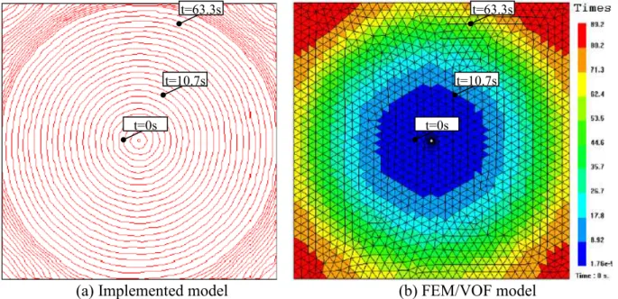
Figure 2 Filling patterns in isotropic radial injection: comparison with analytical solution The same simulation was conducted by activating the gravity contribution. A comparison between the implemented method and a FEM/VOF-based code (PAM-RTM™) is given Figure 3. The same mesh was used for both simulations. As expected, the flow is slightly deported in the lower part of the plate. The predicted filling time is 101s for the implemented model and 89s for PAM-RTM™. The difference is less than 14%, which shows a good qualitative adequacy.

(a) Implemented model (b) FEM/VOF model

Figure 3 Filling patterns: comparison between the implemented model (left) and FEM/ VOF model (right)

Anisotropic injection involving complex shapes. The model was also compared with a more

realistic case. A test was performed consisting of impregnating a 1x1 rib knit fabric made of glass fibers [14] using a canola oil of known viscosity. The preform was placed under a transparent flexible bag and filled using two inlet gates under vaccum conditions (infusion). Front is pulled using two vaccum lines on the upper and lower sides. The dimensions of the mold are given in Fig. 4. Some inserts were placed to assess the contact algorithm. Material and processing parameters are

t=63.3s t=10.7s t=0s t=63.3s t=10.7s t=0s t=10.7s t=63.3s

given in Table 2. CPU time is 200s for a model involving 3693 elements. Data was compared at 0.5s, 3s, 5s and 7s. Figure 6 indicates that agreement is fair at any time. In particular, a front merging is accurately predicted.

Figure 4 Dimensions of the mold Table 2 Material and processing parameters

1

K [m2] K₂ [m2]

µ

[Pa.s]

ε

[-] p_{0 [Pa]} p_f [Pa] r₀ [m] 1.50.10-9 7.75.10-10 0.067 0.705 1.03.105 120 5.10-3

Elapsed time: 0,5s

Elapsed time: 5s

Elapsed time: 3s

Elapsed time: 7s

Conclusion

The presented method is based on combining BEM with Level Set method. Velocity computation is reduced to boundary, which tends to reduce the computational time. An important feature of the method is that the front shape is accurately computed which is more difficult to achieve in standard VOF techniques. Comparing with a Lagrangian approach, the Level Set front tracking facilitates the treatment of topological changes, typically appearing when fronts merge into each other.

Possible extensions of this work may include other physics occurring during the flow (e.g. hydro-mechanical couplings, kinetics). It should be noted that the implemented model includes a gravity term, and can be easily modified to take into account other body forces (inertia effect due to rotation for example). The technique remains similar in three dimensions, considering the resin flow as surfaces propagating.

Acknowledgments

This work was carried out in the framework of FUSCOMP project coordinated by DAHER-Socata. The authors gratefully acknowledge B. Cosson and S. Leroux for their contributions during this work.

References

[1] P. Simacek and S.G. Advani. Composites Part A, 37:1970–1982, 2006.

[2] M-K. Um and L. Wi. Polymer Engineering and Science, 31(11):765–71, 1991.

[3] F.M. Schmidt, P. Lafleur, F. Berthet, and P. Devos. Polymer Composites, 20(6), 1999.

[4] J.A. García, Ll. Gascón, E. Cueto, I. Ordeig, and F. Chinesta. Comput. Methods Appl. Mech. Engrg., (198) 2009.

[5] F. Trochu, R. Gauvin, and D-M. Gao. Adv Polym Technol, 20(6):329–42, 1993;12(4). [6] C. W. Hirt and B. D. Nichols. Journal of Computational Physics, 39:201–225, 1991. [7] J.A. Sethian. Cambridge University Press, 2nd edition, 1999.

[8] S. Soukane and F. Trochu. Composites Science and Technology, 66:1067–1080, 2006. [9] Y-E. Yoo and L. Wi. Polymer Composites, 17(3):368–74, 1996.

[10] K.L. Adams, W.B. Russel, and L. Rebenfeld. International Journal Of Multiphase Flow, 14(2), 1988.

[11] C.A. Brebbia and J. Dominguez. McGraw-Hill Company: Computational Mechanics Publications, 2nd edition, 1992.

[12] E. Mathey. PhD thesis (in French), ENSMP, 2004.

[13] J.A. Sethian and P. Smereka. Annual Review of Fluid Mechanics, 35:341–372, 2003. [14] G. Dusserre, E. Jourdain, and G. Bernhart. Polymer Composites, 2010.