Science Arts & Métiers (SAM)
is an open access repository that collects the work of Arts et Métiers Institute of Technology researchers and makes it freely available over the web where possible.
This is an author-deposited version published in: https://sam.ensam.eu
Handle ID: .http://hdl.handle.net/10985/15336
To cite this version :
Mohamed KEBDANI, Geneviève DAUPHIN-TANGUY, Antoine DAZIN - Modeling dynamic systems : contribution to the unsteady behavior of a condenser based on the pseudo-bond graph approach - International Journal of Modelling and Simulation p.1-18 - 2018
Any correspondence concerning this service should be sent to the repository Administrator : [email protected]
Modeling dynamic systems: Contribution to the Unsteady Behavior of a
Condenser Based on the Pseudo-Bond Graph Approach
M. Kebdani*a, G.Dauphin-Tanguyb, A. Dazina
aArts et Métiers Paris Tech/ LML UMR CNRS 8107, Boulevard Louis XIV, 59000 Lille. France. bEcole Centrale de Lille/ CRIStAL UMR CNRS 9189, CS 20048, 59651 Villeneuve d’Ascq. France.
Abstract
This article is devoted to the dynamic study of the brazed plate condenser (BPC). The proposed model is based on the bond graph theory. The proposed model is based on the bond graph theory because of its energetic approach and multi-physics character of the studied system. The model is discretized into five control volumes. The resolution of mass and energy equations is done by Runge-Kutta method embedded in 20sim software. Analyses of simulation results show that the model has a good ability to transcribe the time evolution of the temperature and pressure in both regimes, transitional and permanent. Also, the model is experimentally validated without any fitting of the set of thermal exchange coefficients.
Keywords: Bond graph theory; Dynamic systems modeling; Multiphysic coupling; Two-phase flow; Heat transfers; Transient; Condenser.
Nomenclature
p
c Specific heat J kg K/ . Thermal conductivity W m K/
h
D Hydraulic diameter m Dynamic viscosity Pa s
e Wall thickness m Density kg m/ 3
G Flow density W Chevron angle degre
H Latent heat of condensation J kg/ f Friction coefficient ---
H Flow enthalpy J/s
g Acceleration m acc Accumulation
l Length m amb Ambiant
L Channels length m col Colector
m Mass kg conv Convection
m Mass flow rate kg s/ dis Distributor
can
N Channels number --- fric Friction
P Pressure Pa in Inlet
Re Reynolds number --- grav Gravity
x Vapor quality liq Liquid
co
p Pitch corrugation m out Outler
Pr Prandtl number --- red Reduced
S Surface m² sat Saturation
t Time s vap Vapor
T Temperature K Difference
1 Introduction
It turns out that the Brazed Plates Condenser (BPC) technology, based on thermal plates with corrugated geometry, allows high performances. This is due to the compact size, and effective heat transfers. These advantages extend the use of BPC. For instance, they equip power electronics cooling systems [1]. A dynamic study of this condenser is necessary to better understand the transitional behavior of this exchanger. Hence the purpose of this article is the development of an original dynamic model based on bond graph approach. The model is experimentally validated using a test rig specially developed for this need.
The article starts with a succinct presentation of the condenser. Afterward, is
presented a state of the art of BPC modeling, convective coefficients correlations and pressure losses correlations. In the second section is given a detailed mathematical description of the proposed thermo hydraulic model. The article ends up with a discussion of experimental results leading to conclude on the validity of the model.
2 General description of a BPC
2.1 Technology and advantages of BPC
The BPC is composed of corrugated plates. The set of thermal plates is brazed with copper, some connections called “ports” are positioned at the corners of the cover plates, see Figure 1. During the brazing operation, the copper is melted and perfectly
conducted to connection points between plates, forming thereby a unique functional block. This process ensures a high level of impermeability and guarantees a structural integrity which allows BPC to withstand important operating pressures up to 45 bar.
Figure 1: Exploded view of a BPC.
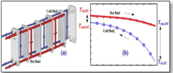
The type of the flow pattern adopted in this work is a counter-current. The two coolants (water) flow in opposite directions, as shown schematically in Figure 2 (a). Indeed, this configuration promotes better heat exchanges, compared to performance provided by a co-current condenser. It is proven that the outlet temperature of the fluid Tout_PC may be lower than the outlet temperature of the secondary Tout SC_ , as shown in Figure 2 (b).
The BPC possesses a number of benefits. They may exist with a volume up to 30% less than that of a traditional tubular condenser [2] and [3]. Also, channel design provides efficient heat transfers. In fact, the multiple fluid streams intersect at the central channel, provoking a turbulent flow [4] and [5], which boosts great heat transfers [6] and [2]. Furthermore, turbulence and secondary flows developed in the exchanger, inhibit the formation of the fouling layers. For more details see [2].
Figure 2: (a) Flow direction of cold and hot fluid in a counter-current BPC
(b) Spatial evolution of the temperature of cold and hot fluids in a counter-current BPC
The BPC is used in a wide range of applications: air conditioning, refrigeration, food and chemical industry. This component is very convenient in monophasic and two phase flow applications. References [2], [5], [6] and [7] contain more details about the different uses of the BPC.
2.2 State of the art on BPC modeling
Unlike tubular condensers, nowadays the scientific literature identifies very few modeling works specific to BPC. On the other side, the majority of disclosed researches works give the main equations used for calculation, important details are not always available. Moreover BPC
dynamic models based on bond graph methodology do not exist in the open literature. Furthermore, the literature revue shows that the dynamic modeling contributions are mainly proprietary of manufacturers and are confidential.
Two examples of works related to BPC
Method of Arman and Rabas [8]: authors developed a stationary model, able to predict the thermo hydraulic state of steam, condensate film and coolant liquid. The BPC iterative model is based on an incremental procedure.
Model of Gut [9]: they present an algorithm allowing the simulation of flow in the steady state. The algorithm is based on the resolution of energy conservation equation. The assumptions are:
the model treats only steady states.
no heat losses to be considered.
the author does not deal with the phase change problems.
the overall heat transfer coefficient is meant to be constant.
the flow is assumed to be “plugged” along the exchanger.
Comparison and scientific contributions Based on the comparison with the existing modeling works, the contributions are:
1. The use of bond graph tool to model the BPC is new. The bond graph is particularly useful in writing the system equations and in assessing the effects of changes in the model even before the equations are written [10] and [11]. 2. The proposed model takes into account
the dynamic behavior, unlike the majority of classical models limited to the permanent regime.
3. The transitional model pays particular attention to the heat transfer coefficients. The novelty, compared to previous work, is twofold: first, coefficients vary with the evolution of local thermodynamic conditions. Second, the thermal behavior of the condenser is experimentally validated without any use of recalibration of the set of used coefficients.
4. Unlike most existing models, the proposed model considers the heat exchange with the outside and the longitudinal conduction along the walls.
5. Gaussian and polynomial correlations of thermo physical properties are specially developed on the basis of data provided by NIST (site 1).
State of the art on the thermal convection coefficients specific to BPCs
The major problems encountered when modeling the BPC are:
- Find out the correct heat transfer coefficients to be used in both primary and secondary circuits.
- Choose the right method to calculate the pressure losses coefficients.
There are no universal and reliable correlations. The reason is due to the strong dependence of coefficients to many parameters such as: plate geometry, mass flow rate, thermo-physical properties of the fluid, vapor quality, pressure and temperature, Reynolds number and dependence of the coefficient hconv on the pattern flow.
Chosen correlations: The scientific literature provides access to a wide range of
heat transfer and friction coefficients. References [12] and [13] present an excellent synthesis work. Nevertheless, we should keep in mind that each correlation remains closely related to the operating conditions under which it has been developed. That is why correlations tested and adapted to our work are given in Appendices B and C.
State of the art on the friction coefficients related to BPCs
The pressure drop in two-phase flows inside a BPC is mainly the sum of three contributions:
• Pressure variation due to gravitation. • Pressure drops at ports.
• Pressure drops due to friction of the two-phase flow.
This section aims at presenting the pressure losses correlations applied for two-phase flows.
Pressure variation due to gravitation: the change in pressure due to gravity is determined by the hydrostatic equation:
grav aver
P g L
( 1 )
where the average density aver of the two phase flow is given by:
1 1 aver vap liq x x ( 2 )
Pressure drop in distributors and collectors: the losses generated inside distributors (inflow) and collectors (outflow) are empirically estimated by Shah and Focke [3]: 2 / 1.5 2 col dis aver G P ( 3 )
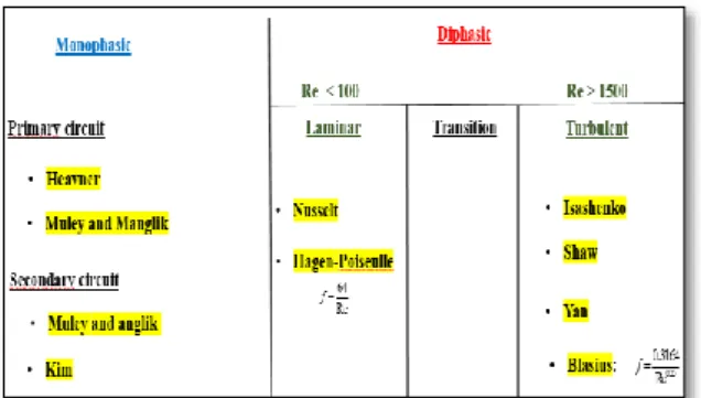
Pressure losses due to friction of the phase flow: the friction coefficient in two-phase flow is complicated to determine. The Table 2 shows a number of correlations available in the literature.
Chosen correlations: The correlations feeding the proposed model are chosen as follows:
Figure 3: Classification of correlations in function of flow regime.
3 Bond graph model of the BPC.
3.1 About the theory of bond graphs
Industrial thermo fluids systems are multidisciplinary. Their functioning involves systematically several domains of the physic (mechanic, hydraulic, thermal, chemical, and electrical fields). This phenomenological complexity makes it difficult to develop a standard model based on partial derivative equations (CFD1). The bond graph methodology is based on differential equations. It allows to represent graphically the power exchanges between components of a complex system. A bond graph model is a unified graphical representation for all areas of engineering science. It is based on the principle of analogy between different fields of physics [14] and [15]. Also, a bond graph model is both structural and behavioral which allows simulation and analysis of the model properties [16]. The bond graph allows modeling adapted to the growing technological needs. In fact, the model can be easily modified by adding or removing elements, permitting a modeling approach called ‘bottom-up’ or ‘top down’.
3.2 Assomptions
The model is based on the following hypotheses:
The fluid is unidirectional.
The fluid in the secondary circuit (SC) flows with a constant mass flow rate.
1 CFD: Computational Fluid Dynamics
The two-phase volume connoted V6 in
Figure 5 occupies half of the primary circuit volume (PC).
The refrigerant used for the simulation is water, while the validation tests are conducted with water containing 4% of PAG2
The temperature gradient in the condensate film is assumed to be linear: this hypothesis is plausible given the small hydraulic diameter of channels.
3.3 Control volumes
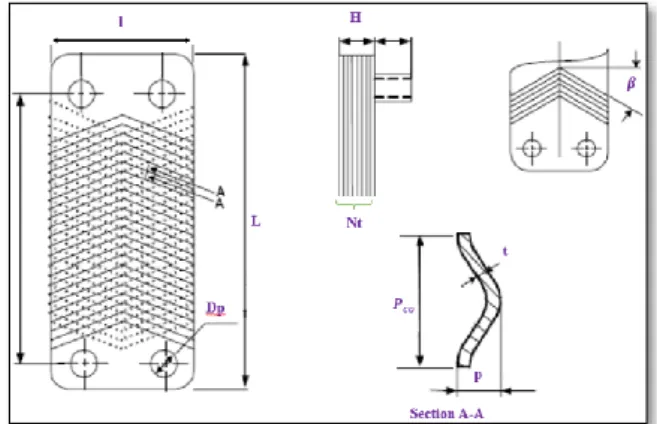
The BPC is composed of channels in both circuits: hot, called primary circuit (PC), and the cold one also called secondary circuit (SC), as shown in Figure 4.
Figure 4: internal geometry of flow channels in a BPC.
In our modeling work the BPC is the union of six control volumes:
Figure 5: Volume discretization of the BPC, and distribution of heat flows occurring during the
condensation phenomenon.
The primary circuit (PC) is assimilated to
a simple pipe. In case of two-phase flow, the PC is divided into two volumes separated by a condensation interface as shown Figure 5:
V6 a diphasic flow: homogeneous mixture of liquid and vapor.
V5 a monophasic flow: constituted of condensate film and the liquid “drained” down the condenser.
The secondary circuit (SC) has a cylindrical form and contains water in single phase state. This circuit is represented by two volumes V3 and V4 as shown in Figure 5.
The material body of the condenser is represented by two volumes V1 and V2.
3.4 General structure of the bond graph model.
The structure of the bond graph model is shown in Figure 6. The six sub models shown in Figure 6 refer to the six volumes mentioned above and are represented by the following bond graph elements:
Volume designation Bond graph
element V1 and V2 outer wall of the
BPC
C elements with 1 thermal port V3 and V4 Secondary circuit
RC elements with 2 ports (thermal and hydraulic). V5 liquid portion occupying the primary circuit RC element with 2 ports (thermal and hydraulic). V6 two-phase portion present in the primary circuit C element with 2 ports (thermal and hydraulic).
Blue lines correspond to the hydraulic power exchanges, while the orange lines represent the thermal power transfers. All studied heat transfer phenomena (convection and conduction) are modeled by dissipative elements
3.5 Mathematical description of the dynamic bond graph model
A detailed description of conservation equations (mass and energy) governing the thermo hydraulic behavior of the condenser is proposed here. The resolution of the equations is done by Runge-Kutta method embedded in 20sim software (site 2). The chosen "effort / flow" variables are pressure
and mass flow rate for hydraulic domain and temperature and enthalpy flow (for convection) or heat flow (for conduction) for thermal domain. This is why the proposed model is a pseudo bond graph. Moreover it is possible to use volume flow rate [17] and entropy flow rate instead of mass flow rate and enthalpy flow rate to build a real Bond Graph, however the mathematical formalism will be more complicated. Note, that interpolations giving the evolution of thermo physical properties are specifically developed for the current project with high accuracy, and are given in [18].
Volume V1 of the outer wall
The temperature TV1( )t is calculated using the energy balance. Furthermore, this volume is submitted to two thermal flows, as shown in Figure 5, HV3/ 1V modeled in bond graph by
_ 1_
Wall V INT
R and HV1/amb modeled by the element
_ 1_
Wall V EXT
R . The energy balance is written at
the 05 junction:
_ 1_ 3/ 1 1/
Wall V acc V V V amb
H H H ( 4 )
The enthalpy stored inside V1 is then
calculated in the element CWall V_ 1 as: _ 1_ ( ) _ 1_ ( ) _ 1,0
Wall V acc Wall V acc Wall V t
H t H t dtH ( 5 )
where, HWall V_ 1,0 is the initial enthalpy in the wall V1.
The constitutive law of the element CWall V_ 1 giving the temperature of the wall is then:
_ 1_ 1 1 , 1 ( ) . Wall V acc V V p V H T t m c ( 6 ) , 1 p V
c : Specific heat of the wall (inox316).
Volume V2 of the outer wall
The temperature TV2( )t inside the volume V2 is obtained in a similar way from the constitutive law of the element CWall V_ 2
_ 2 _ 2 2 , 2 ( ) . Wall V acc V V p V H T t m c ( 7 ) with: cp V, 2cp V, 1416 ( /J kg K. ) et mV2mV1.
Figure 6: Dynamic bond graph model of the BPC.
Volume V3 of the liquid in the CS Mass conservation equation
The coolant mass flow rate min V_ 3 is considered constant. Which means that there is no mass storage in the volume V3. Energy balance equation
The energy balance is written in the 03
junction: _ 3 _ 3 _ 3 5/ 3 3/ 1 _ 3 3 _ 3 in V acc V in V V V V V s V V liq V m H H H H H P (8)
The enthalpy stored in V3 is then calculated
in the element RCLiq V_ 3 as: _3( ) _ 3( ) _ 3,0
acc V acc V liq V t
H t H t dtH ( 9 )
where, Hliq V_ 3,0 is the initial enthalpy in the wall V3. The constitutive law of the element
_ 3
Liq V
RC giving the temperature of the wall is
then: _ 3 3 _ 3 , , 3 ( ) ( ) 2 acc V V in V p liq V H t T t m c ( 10 )
The pressure drop PV3 modeled by the 2-ports element RCLiq V_ 3 is obtained using equations: ( 11 ), ( 12 ), ( 13 ) and ( 14 ). Frictional pressure losses induced in single phase flow Pfric are calculated using Darcy- Weisbach formula.
3 /
V grav fric col dis
P P P P ( 11 ) where : _ 3 3 grav liq V V P g L ( 12 ) 2 / 1.5 2 col dis m G P ( 13 ) 2 _ 3 2 3 _ 3 3 _ 3 1 2 2 ² in V V fric liq V h liq V h m L P v f f D D ( 14 )
If : Re100 (laminar regime according to
Wanniarachchi [5]), then Hagen- Poiseuille formula is used:
64 Re
If not (transient or turbulent regime), the formula of Blasius for turbulent flow regime gives:
0.25
0.3164 Re
f ( 16 )
Now it remains to determine the hydraulic diameter: Dh. For a better understanding of the geometric problem, parameters used in the formula ( 17 ) are denoted in Figure 7.
3 3 4 4 2 2 V h V S b l b D Per l ( 17 ) with :
1.17, a value given by the
manufacturer SWEP.
b p t. Where “p” is the corrugation
depth and “t” the corrugation thickness.
Figure 7: Specification of geometric parameters on the thermal plate of a BPC.
Volume V4 of the liquid in the CS The liquid temperature is calculated as:
_ 4 4 _ 4 , , 4 ( ) ( ) 2 acc V V in V p liq V H t T t m c ( 18 )
Volume V5 of the liquid in the PC
As long as the liquid temperature does not exceed the saturation temperature corresponding to the pressure in the volume V5, the condenser contains only the liquid phase. Henceforth, a phase indicator is defined as follows:
if Tliq V_ 5Tsat(Pevap) : then the fluid is liquid in a single-phase state ( no vapor trace exists in the liquid) and indPC0. In this case, the whole PC is modeled only by
the element RCLiq V_ 5 while the element _ 6
Diph V
C has no physical impact.
if Tliq V_ 5Tsat(Pevap), then: indPC1. It is assumed that the total volume of the PC is divided into two equal volumes V5 and V6, successively represented by the elements: RCLiq V_ 5 and CDiph V_ 6.
Case I: indPC0 : PC, containing only liquid, is modeled by the element: RCLiq V_ 5.
Mass conservation equation
During the single-phase flow it is assumed that the mass flowrate mout V_ 5 of the refrigerant through the PC is constant. Energy balance equation
The energy balance is written in the 01
junction:
_ 5
_ 5 _ ( ) / 5/ 3 _ 5 5
_ 5
out V acc V in CP mono Diph Liq V V out V V
liq V
m
H H H H H P
(19)
The enthalpy stored within V5 is then
calculated in the element RCLiq V_ 5 as: _ 5( ) _ 5( ) _ 5,0
acc V acc V liq V t
H t H t dtH ( 20 )
where, Hliq V_ 5,0 is the initial enthalpy in the volume V5.
The constitutive law of the element RCLiq V_ 5 giving the temperature of the wall is:
_ 5 5 _ 5 , _ 5 ( ) ( ) acc V V out V p liq V H t T t m c ( 21 )
The pressure drop PV5 in the volume V5 represented by the multiport element RCLiq V_ 5 is calculated like PV3.
Case II: indPC1: the liquid volume V5 is modeled by the element : RCLiq V_ 5. Equations specific to RCLiq V_ 5 are identical to those presented in the case above, but with a volume V5/ 2 and a pipe lengthLV5/ 2.
Volume V6 of the two-phase mixture The two-phase volume V6 constituted of
half the total volume of the PC, is modeled by the element CDiph V_ 6 whose mathematical description is:
Mass conservation equation:
This equation is written in the thermal 0h2
junction
_ 6 _ 6
acc V in V cond
m m m ( 22 )
min V_ 6 is the mass flow rate of the fluid entering into the condenser. It is calculated by solving the momentum equation at the condenser inlet.
The condensate mass flow rate mcond in the condenser is established in [18]. Its expression is:
3
2
3 2
liq vap film h
cond liq liq g D m ( 23 ) 1/4
4 liq liq / 2 wall vap film
liq liq vap
L T T g H ( 24 )
The mass stored in the volume V6 is
calculated in the multiport element CDiph V_ 6 as:
_ 6( ) _ 6( )
acc V acc V t
m t m t dt ( 25)
Energy balance equation
The energy balance is written in the 0t2
junction:
_ 6 _ 6( ) / 6/ 4
acc V in V diph Diph Liq V V
H H H H ( 26 )
The enthalpy stored inside V6 is then
calculated in the element CDiph V_ 6 as: _6( ) _6( )
acc V acc V t
H t H t dt ( 27 )
The constitutive laws of the element CDiph V_ 6 giving the pressure PV6 and the temperature
6
V
T of the two-phase flow are the result of a
complex mathematical calculation that requires, at each time step, a connection between Matlab and 20sim. The connection is meant to solve a polynomial equation of 12th order whose solution is the pressure of the two-phase mixture. On the other hand, this method detailed in appendix A is able
to predict the temporal evolution of the vapor quality x t( ) of the two-phase mixture. Temperature of the two-phase mixture: this temperature is obtained directly from
the pressure PV6( )t , since it is assumed that the vapor-liquid mixture is saturated. Pressure and temperature are related by the following interpolation, especially developed for the project:
2 6 6 2 6 2 6 1.078 367.5 1.081 0.173 125 0.4797 ( ) ( ) e 0.03264 3 x 8.8 p ( ) exp 7 0. ( ) e 19 7 x 6 p V V V V P t T t P t P t ( 28 ) 3.6. Expression of conducto-convective flows
Heat flows are modeled using dissipative R-elements, used formula are listed in Appendix D: Conduction flows. According to Newton formula we have:
conv ech
h S T
( 29)
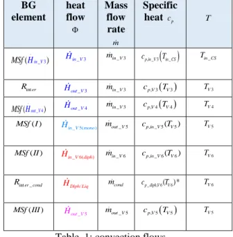
Convected enthalpy is : m cp T, with:
BG element heat flow Mass flow rate m Specific heat cp T . _ 3 ( in V) MSf H Hin V_ 3 min V_ 3 cp in V, _ 3 Tin CS_ Tin CS_ int er R _ 3 out V H min V_ 3 cp V, 3 TV3 TV3 . _ 4 ( out V) MSf H Hout V_ 4 min V_ 3 cp V, 4 TV4 TV4 ( ) MSf I Hin V_ 5(mono) mout V_5 cp in V, _ 5(TV5) TV5 ( ) MSf II _ 6( ) in V diph H min V_ 6 cp in V, _ 6(TV6) TV6 inter cond_
R HDiph Liq/ mcond cp diph V_ , 6(TV6)* TV6
( )
MSf III
_ 5 out V
H mout V_5 cp V, 5 TV5 TV5 Table 1: convection flows.
where :cp diph V_ , 6(TV6)* x cp vap, TV6 (1 x c) p liq, TV6
4 Experimental validation
4.1 Sensors
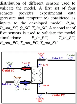
The Figure 8 gives a schematic representation of the BPC, as well as the
distribution of different sensors used to validate the model. A first set of four sensors provides experimental data (pressure and temperature) considered as inputs to the developed model: P_in, P_out_SC, Q_SC, T_in_SC. A second set of five sensors is used to validate the model simulations: P_in_PC, T_in_PC, P_out_PC, T_out_PC, T_out_SC.
Figure 8: Position of pressure, temperature and mass flow sensors mounted on the BPC.
All geometric data required to launch a simulation are reported in Appendix E.
Description of the validation test
The three experimental data (Pin, SC SC liq Q m _ in SC
T ) represent the boundary conditions
applied to the condenser and are plotted in Figure 9. The pressure Pout_SC is atmospheric. The test is composed of four steps reported in Figure 9:
The interval referenced II in the Figure 9 corresponds to the heating of the refrigerant moving through the condenser. During this phase, the fluid heats up but remains liquid.
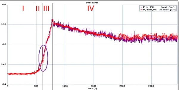
The beginning of interval III is marked by a sudden peak of pressure Pin
(highlighted by a circle). Indeed, this peak reflects the birth of vapor bubbles.
Furthermore, the pressure Pin is fluctuating throughout intervals III and
IV. These oscillations are due to the
presence of vapor bubbles.
During interval IV the circulation of the coolant fluid contained in the secondary circuit is triggered. The corresponding mass flow rate m_dotSC is given by graph 2.
The model validation is based on comparison of the time evolution of simulated and measured values of: temperatures and pressures in volumes: 5V (liquid) and 6V (two-phase mixture), shown schematically in Figure 5.
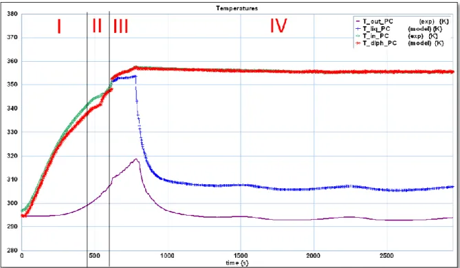
Figure 10: Time evolution of the temperatures calculated in the condenser and measured at the terminals
4.2 Temperatures
Figure 10 gives the time evolution of:
Liquid temperature, measured at the condenser outlet: Tout_PC.
Liquid temperature, calculated inside the volume V5 of the condenser: T_liq PC_
Temperature of the mixture, measured at the condenser inlet: Tin PC_ .
Temperature of the mixture, calculated inside the volume V6 of the condenser:
_diph PC_
T .
Monophasic intervals (I and II)
Firs, it should be noted that the temperature of the mixture T_diph PC_ is considered equal to the liquid temperature T_liq PC_ as long as the two-phase flow does not appear (indPC0). Generally, during this heating phase, it is found that the global dynamic translated by the calculated temperature T_liq PC_ is very similar to that one measured in the condenser inlet Tin PC_ .
However, discrepancies remain between the two quantities. Actually the temperature sensor Tin PC_ , see Figure 8, is mounted at the input port of the condenser, while the liquid
temperature T_liq PC_ is calculated in the primary circuit represented by the volume V5, see Figure 5. This difference is then justified by the temperature gradient existing between the measurement point and the calculation volume.
The temperature difference between the condenser outlet Tout_PC and T_liq CP_ can be explained:
The temperature sensor is positioned on the outer wall of the pipe connected to the condenser outlet. Then, the temperature gradient in the wall is not negligible.
The sensor is not thermally insulated from the outside. Therefore, it is obvious that the measurement of this temperature is disturbed by convective heat exchange with ambient air.
Finally, the sensor used has an accuracy of 1.5 ° C.
Diphasic intervals (III and IV)
Once the two-phase behavior occurs, the condenser model is treated as two volumes, separated by a condensation interface, see
Figure 5. This justifies the presence of two calculated temperatures: T_diph PC_ and T_liq PC_ . In two-phase state, water is saturated, so its temperature is a function of the pressure. However, the pressure at the inlet of the condenser, just in front of the temperature sensor Tin PC_ , is close to that prevailing inside the condenser (volume V6 of Figure 5), the small difference is due to low pressure drop. Therefore, the measured temperature of the diphasic mixture Tin PC_ and the calculated temperature T_diph PC_ are meant to be very close, which is found by the transient model
(red curve compared to the green one in Figure 10).
As to the liquid temperature T_liq PC_ , the thermal dynamics translated by the temperature sensor is retrieved. However, the discrepancies are due to the sensor position. Also, once the fluid in the secondary circuit flows, the model predicts a decrease of the liquid temperature T_liq PC_ with a correctly estimated slope. Finally, required time to reach the second steady regime seems to be the same for the model as for the experiment.
Figure 11: Time evolution of the liquid pressures, calculated and measured in the BPC.
4.3 Fluid pressure in the primary circuit
The time evolutions of the liquid pressure, calculated P_liq PC_ and measured Pout_PC are shown in Figure 11. While the pressure of the diphasic mixture, calculated P_diph PC_ and measured Pin PC_ are plotted in Figure 12. Pressures P_liq PC_ and P_diph PC_ are well transcribed by the transient model in both states: steady and transient which highlights the ability of the model to predict, with good accuracy, the transition from single-phase to two-phase regime. This transition is controlled using the phase indicator introduced in paragraph (3.5).
Result of the validation test
Comparison between simulation results and experimental data reveals that the dynamic model is able to predict, with good agreement, the thermo hydraulic dynamic of the brazed plate heat exchanger. Despite the modeling simplification hypotheses, the model does not react as a low pass filter and allows the identification of unsteady phenomena.
5 Conclusion
The article starts with a succinct description of the brazed plates condenser. It turns out that the technology based on corrugated plates, gives to the exchanger competitive performances. This is due to its compactness, and efficient heat transfers which explain the wide use of this exchanger, particularly in cooling loop used in space applications and constituting the heart of our works.
In the first section two literature reviews have been conducted. The first one, devoted to study existing models, is used to highlight the originality of the proposed model. The second one allows establishing a synthesis of correlations related to thermal convection coefficient and pressure losses, classically used for the two regimes: monophasic and biphasic.
The second section describes the mathematical model of BPC. The model is based on the bond graph methodology. The modularity of this approach gives the model an evolutionary feature, where it is possible to rewrite equations (for a finer modeling) without changing the original structure. The model is discretized into five volumes and is based on the resolution of mass and energy conservation equations. Finally, modeling of heat exchanges is engaged with a noticeable attention. Indeed, the model is validated using several tests without any experimental recalibration of exchange coefficients.
A final section is devoted to the comparison of the simulation results obtained by the unsteady model with experimental recordings from the test bench. An analysis of modeling results leads to conclude that the model has a good ability to transcribe the time evolution of temperatures and pressures, in both regimes, transitional and permanent.
Acknowledgment
This Article describes results from researches supported by the FUI 14 Program in the context of project ThermoFluid RT labeled by the competitively pole ASTech. The authors wish to express their gratitude to Mr. R. Albach from Atmostat and Mr Raymond Peiffer, responsible of Thermal analysis from MBDA missils for the multiple fruitful scientific discussions about innovative technologies.
Disclosure statement
No potential conflict of interest was reported by the authors.
References
[1] M. Kebdani, G. Dauphin-Tanguy, A. Dazin, and P. Dupont, “Bond Graph Model of a mechanically Pumped Biphasic Loop (MPBL),” in 23rd Mediterranean Conference on
Control and Automation (MED), 2015, pp. 448–453.
[2] R. Eldeeb, V. Aute, and R. Radermacher, “A Model for Performance Prediction of Brazed Plate Condensers with Conventional and Alternative Lower GWP Refrigerants,” in 15 th international Refrigeration and Air Conditioning Conference, 2014, pp. 1–10.
[3] G. A. Longo, “R410A condensation inside a commercial brazed plate heat exchanger,” Exp. Therm. Fluid Sci., vol. 33, no. 2, pp. 284–291, 2009.
[4] M. H. Maqbool, “Flow boiling of ammonia and propane in mini channels,” Royal Institute of Technology, (KTH) Stockholm, Sweden, 2012.
[5] S. Muthuraman, “The Characteristics of Brazed Plate Heat Exchagers with Different Chevron Angles,” Glob. J. Res. Eng., vol. 11, no. 7, pp. 11–26, 2011.
[6] L. Cremaschi, A. Barve, and X. Wu, “Effect of Condensation Temperature and Water Quality on Fouling of Brazed-Plate Heat Exchangers.,” ASHRAE Trans., vol. 118, no. 1, pp. 1086–1100, 2012. [7] P. Vlasogiannis, G. Karagiannis, P.
Argyropoulos, and V. Bontozoglou, “Air – water two-phase flow and heat transfer in a plate heat exchanger,” Int. J. Multiph. Flow, vol. 28, no. 5, pp. 757–772, 2002.
[8] B. Arman and T. J. Rabas, “Condensation analysis for plate-frame heat exchangers,” in National Heat Transfer Conference, 1995, vol. 314, no. 12, pp. 97–104.
[9] J. A. W. Gut, R. Fernandes, J. M. Pinto, and C. C. Tadini, “Thermal model validation of plate heat exchangers with generalized configurations,” Chem. Eng. Sci., vol. 59, no. 21, pp. 4591–4600, 2004. [10] S. Azarbaijani and D. Karnopp, “Pseudo Bond Graph Structural Models for Heat Exchangers,” Int. J. Model. Simul., vol. 2, no. 3, pp. 138– 141, 1982.
[11] M. Kebdani (b), G. Dauphin-Tanguy, A. Dazin, and P. Dupont, “Experimental development and bond graph modeling of a Brazed-Plate Heat Exchanger (BPHE),” Int. J. Simul. Process Model., vol. 12, no. 3/4, pp. 249–263, 2017.
[12] L. Wang, B. Sundén, and R. Manglik, “Plate Heat Exchangers: Design, Applications, and Performance,” WIT Press, pp. 8–45, 2007.
[13] Z. H. Ayub, “Plate Heat Exchanger Literature Survey and New Heat Transfer and Pressure Drop Correlations for Refrigerant Evaporators,” Heat Transf. Eng., vol. 24, no. 5, pp. 3–16, 2003.
[14] W. Borutzky, Bond graph modelling of engineering systems, Springer. 2011.
[15] D. Singer, “Bond graph modelling-a general system theory approach,” Int. J. Gen. Syst., vol. 18, no. 1, pp. 23– 35, 1990.
[16] G. Dauphin-Tanguy, A. Rahmani, and C. Sueur, “Bond graph aided design of controlled systems,” Simul. Pract. Theory, vol. 7, no. 5–6, pp. 493–513, 1999.
[17] A. Singh and T. K. Bera, “Bond graph aided thermal modelling of twin-tube shock absorber,” Int. J. Model. Simul., vol. 36, no. 4, pp. 183–192, 2016.
[18] M. Kebdani (a), G. Dauphin-Tanguy, A. Dazin, and R. Albach, “Two-phase reservoir: Development of a transient thermo-hydraulic model based on Bond Graph approach with experimental validation,” Math. Comput. Model. Dyn. Syst., vol. 23, no. 5, pp. 476–503, 2016.
[19] A. Muley and R. M. Manglik, “Enhanced Heat Transfer Characteristics of Single-Phase Flows in Plate Heat Exchangers with Mixed Chevron Plates,” Enhanc. Heat Transf., vol. 4, no. 3, pp. 187– 201, 1997.
[20] Y. Y. Yan, H. C. Lio, and T. F. Lin, “Condensation Heat Transfer and Pressure Drop of Refrigerant R- 134a in a Plate Heat Exchanger,” Int. J. Heat Mass Transf., vol. 42, no. 6, pp. 993–1006, 1999.
[21] W. S. Kuo, Y. M. Lie, Y. Y. Hsieh, and T. F. Lin, “Condensation Heat Transfer and Pressure Drop of Refrigerant R-410A Flow in a Vertical Plate Heat Exchanger,” Int. J. Heat Mass Transf., vol. 48, no. 25– 26, pp. 5205–5220, 2005.
[22] A. Muley and R. M. Manglik, “Experimental study of turbulent flow heat transfer and pressure drop in a plate heat exchanger with chevron plates,” J. Heat Transf. ASME, vol. 121, no. 1, pp. 110–117, 1999.
[23] D. Han, K. Lee, and Y. Kim, “The Characteristics of Condensation in brazed Plate Heat Exchangers with Different Chevron Angles,” J.
Korean Phys. Soc., vol. 43, no. 1, pp. 66–73, 2003.
[24] W. Nusselt, “The Condensation of Steam on Cooled Surfaces.,” Chem. Eng. Fundam., vol. 1, no. 2, pp. 6– 19, 1982.
[25] R. Sánta, “The Analysis of Two-Phase Condensation Heat Transfer Models Based on the Comparison of the Boundary Condition,” Int. J. Acta Polytech. Hungarica, vol. 9, no. 6, pp. 167–180, 2012.
Appendix A: Mathematical formalism Graphical scheme of the pressure calculation:
Figure 13: P-h diagram of Mollier.
Theoretical developments
Specific enthalpy of the two-phase mixture:
_ 6 6 _ 6 ( ) ( ) ( ) acc V V acc V H t h t m t ( 30 )
Specific volume of the two-phase mixture
6 _ 6 6 ( ) ( ) V acc V V v t m t ( 31 )
Construction of the 12 order polynomial
The specific volume vV6( )t of the mixture can also be expressed as:
"
6( ) ( 6( )) (1 ) '( 6( ))
V V V
v t x v P t x v P t ( 32 )
The specific enthalpy hV6( )t of the mixture can be expressed as:
"
6( ) ( 6( )) (1 ) '( 6( ))
V V V
h t x h P t x h P t ( 33 )
Note about the thermodynamic functions:
"
v , "
h v' and h' are respectively the specific volume
and enthalpy of the vapor portion in the mixture and specific volume and enthalpy of the liquid portion in the mixture. These four thermodynamic functions are all expressed in terms of the pressure PV6( )t using polynomial interpolation. From the two equations ( 32 ) and ( 33 ), and some other arrangements, we are able to get the 12-order polynomial equation ( 34). The real, positive and minimum root of this equation is the researched pressure PV6( )t
6 6 " ' 6 6 6 0 0 6 6 " ' 6 6 6 0 0 6 6 ' " 6 6 6 0 0 ( ) ( ) ( ) ( ) ( ) ( ) ... ( ) ( ) ( ) i i V i V i V i i i i i V V i V i i i i i V i V V i i v t h P t h P t v P t h t h P t v P t h P t h t 0 ( 34)
Vapor quality of the two-phase flow
The resolution of the equation ( 34) provides, at each time step, a value of the pressure PV6( )t . Based on this value, determining the Vapor quality becomes easy: 6 " 6 , 6 0 6 6 ' " , 6 , 6 0 0 ( ) ( ) ( ) ( ) ( ) i V i j V i i i i j V i j V i i v t v P t x t v P t v P t ( 35 )
Appendix B: friction coefficients
Author Comments formula
Muley and Manglik
[19]
Valid for water. For Prandtl : Pr2.4; 4.5 0.2 5 5 0.5 0.15 Re 2; 200 40.32 8.12 Re Re Re 1000 1.274 Re f f
Darcy Weisbach Valid for water
Hagen- Poiseuille for laminar flow
64 Re
f Blasius for turbulent flow
0.25
0.3164 Re
f
Table 2: Friction coefficients correlations used for single-phase flow.
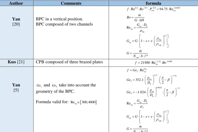
Author Comments formula
Yan [20]
BPC in a vertical position. BPC composed of two channels
0.4 0.5 0.8 0.0467 1/2 Re 94.75 Re Re 1 * red eq eq h eq liq liq eq vap can f Bo P m Bo G H G D G G x x m G N b l
Kuo [21] CPB composed of three brazed plates 1.14 0.085
21500 Reeq
f Bo
Yan [5]
3
Ge and Ge4 take into account the geometry of the BPC.
Formula valid for: Reeq300; 4000
4 3 4.17 7.75 3 0.0925 1.3 4 1/2 Re 352.1 2 1.024 2 Re 1 * Ge eq co h co h eq h eq f liq eq vap can f Ge p Ge D p Ge D G D G G x x m G N b l
Appendix C: heat transfer coefficients
Author Comments formula
Heavner [19]
Valid for water.
0.17 1/3 Re Pr m wall Nu J b Boyko and Kruzhilin (Sánta 2012)
Valid for water.
0.8 0.43
0.0021 Re Pr liq
conv liq liq h h D Muley and Manglik [22]
Valid for water.
Pr 5;10 Re 200;1200 eau eau 0.766 0.333 0.277 liq Re Pr
conv liq liq
h h D Kim
[23] Valid for water.
0.09 0.64 0.32 0.295 Re Pr 2 liq conv h h D
Table 4: Correlations of heat transfer coefficients used for single-phase flow.
Author Comments formula
Nusselt [24] Laminar film. Condensation controlled by gravity. Vertical surface.
Linear temperature gradient in the film.
Constant Steam temperature.
1/4 2 3 4 * liq liq conv
liq sat wall
g H h l T T Boyko And Kruzhilin [25]
Takes into account water vapor. Valid for Reynolds number:
Re1500;15000
Valid for annular flow.
0.8 0.43
0.5 0.021 Re Pr
1 1
f liq liq liq
h liq conv liq vap D h x Shaw [12] Condensation controlled by shearing.
Valid for water vapor.
0.8 0.76 0.04 0.8 0.4 0.38 3.8 1 0.023 Reliq Prliq 1 red red crit liq conv h x x Nu x P P P P Nu h D
Appendix D: Conduction flows
BG element heat flow: Convection coefficient hconv Exchange surface ech S T _ 1_ Paroi V INT R HV3/ 1V Alfa Laval : 0.3274 3 1/3 234 liq Pr liq V liq P Nu 3 V P
Pressure drop in (kPa)
liq
: Viscosity in (cP).
2 l L The liquid in the SC
exchanges with the ambient through the
two cover plates.
3 1 V V T T _ 1_ Paroi V EXT R HV1/amb 0.25 1 1.42 / 2 V amb ext T T h L 2 l L TV1Tamb _ 2 _ Paroi V INT R HV4/ 2V 0.3274 3 1/3 234 Pr liq V liq liq P Nu PV4:
Pressure drop in (kPa)
liq : viscosity en (cP). 2 l L TV4TV2 _ 2 _ Paroi V EXT R HV2/amb 0.25 1 1.42 / 2 V amb ext T T h L 2 l L TV2Tamb _ Liq Liq R HV5/ 3V 5 3 1 1 1 conv wall wall V V h e h h
Boyko and Kruzhilin : 0.8 0.43 5 0.021 Re5Pr5 liq V V V h h D Alfa Laval : 0.3274 3 1/3 3 234 Pr liq V V liq liq liq P h 0.0240 ²m
Value given by the manufacturer of BPC
used in this work.
5 3 V V T T _ Diph Liq R HV6/ 4V 5 6 1 1 1 conv wall wall V V h e h h
Boyko and Kruzhilin : 0.8 0.43 6 6 0.5 6 0.021 Re Pr 1 1 liq f V V h liq V f vap D h x 0.0240 ²m
Value given by the manufacturer of BPC
used in this work.
6 4
V V
T T
Table 6: Modeled conduction flows.
Appendix E: Geometric parameters of the BPC
Parameter notation value Parameter notation value
Number of plates
t
N 6 Volume of SC VCS 0.0741 dm3
Plate Thickness t 0.0003 m Volume of PC VCP 0.0494 dm3
Plate Length L 0.154 m Exchange surface Sech 0.048 m².
Plate Height H 0.0174 m material Inox 316
Plate Width l 0.076 m Pitch of
corrugation co p 0.001 m Angle of chevron 30° Total number of channels 1 can t N N 5


![[PDF] Guide Visual Basic : initiation a la programmation evenementielle | Cours visual basic](data:image/gif;base64,R0lGODlhAQABAIAAAP///wAAACH5BAEAAAAALAAAAAABAAEAAAICRAEAOw==)