Analysis of Indirect Measurement of Cutting Forces Turning Metal Cylindrical Shells

Science Arts & Métiers (SAM)

is an open access repository that collects the work of Arts et Métiers Institute of Technology researchers and makes it freely available over the web where possible.

This is an author-deposited version published in: https://sam.ensam.eu

Handle ID: .http://hdl.handle.net/10985/10634

To cite this version :

Kirill KONDRATENKO, Alexander GOUSKOV, Mikhail GUSKOV, Philippe LORONG, Grigory PANOVKO - Analysis of Indirect Measurement of Cutting Forces Turning Metal Cylindrical Shells - In: VETOMAC X, Royaume-Uni, 2014-09-09 - Vibration Engineering and Technology of

Machinery - 2015

Any correspondence concerning this service should be sent to the repository Administrator : archiveouverte@ensam.eu

forces turning metal cylindrical shells

1. Bauman Moscow State Technical University, Department RC5, Moscow, Russia. 2. National Research Centre “Kurtchatovsky Institute”, Moscow, Russia.

3. ENSAM-ParisTech, Paris, France. 4. IMASH RSA, Moscow, Russia.

Email: kk92@ya.ru, gouskov_am@mail.ru, mikhail.guskov@ensam.eu,

philippe.lorong@ensam.eu, gpanovko@yandex.ru.

Abstract Cutting forces measurement is an important component of the ma-chining processes development and control. The use of conventional direct meas-urement systems is often impossible as they interfere in the process’s dynamics. This work proposes a method of cutting force indirect estimation during turning thin-walled cylindrical shells. Calculation of the flexibility matrix has enabled us to relate measured displacements of certain workpiece’s points to the cutting force. An optimization approach for choosing the measurement points location has been proposed, based on the best conditioning of the flexibility matrix.

Key words Cutting forces measurement, Thin-walled workpiece, Technological system, Optimization, Ill-conditioned systems.

1.0 Introduction

In modern manufacturing, cutting forces measurement is a key element in under-standing the operational conditions during machining workpieces. Usually, cutting forces are measured directly using different kinds of dynamometers. For instance, in [1], an experimental set-up is described where cutting forces are measured di-rectly, with a Kistler 9257B three-component piezo-dynamometer. The direct measurement approach is also incorporated in [2]. Another approach, based on the use of currents drawn by a.c. feed-drive servo motors, is presented in [3], where the pulsating milling forces are measured indirectly within the bandwidth of the current feedback control loop of the feed-drive system.

Nevertheless, in some cases, the use of dynamometers can be problematic, for in-stance in case of thin-walled workpieces in presence of instabilities: due to the presence of resonances in the frequency response of the dynamometer can induce

2

significant perturbations in the measured signals. This was the case for [4]: the ad-dition of the dynamic system of the dynamometer has modified the conad-ditions of the chatter onset.

In the present paper, we address the problem of quasi-static evaluation of the cut-ting force during turning cylindrical shells. The cutcut-ting force components are es-timated indirectly, from the displacement measurements, with the help of the flex-ibility matrix, based on the elastic behavior of the structure.

Fig. 1 The components of the cutting force (on the left). The free end of the shell (on the right) with angular location of the displacement sensors shown.

Two arbitrary points belonging to the free end of the shell are chosen: point and . The points represent the location of two displacement sensors. The angular lo-cation of these points is determined by parameters Φ and Φ , which is shown in Fig. 1. The radial displacements of these points are actually measured using non-contact displacement sensors. The relation between the two components , of the cutting force and the radial displacements and of points and at first approximation is linear and injective:

=

where

= , = , = . (2)

Matrix is called the flexibility matrix. Parameter Λ determines the axial position of the cutting force. In order for the solution = to be reliable, system (1) has to be numerically stable. The system stays numerically stable as long as its condition number is sufficiently close to 1.The question of the optimality of the sensors position is sought in terms of the condition number of the flexibility ma-trix.

Section 2 addresses the algorithm of calculation of the flexibility matrix, and Sec-tion 3 describes a particular way of avoiding numerical instabilities calculating this matrix.

2.0 Calculation of the Flexibility Matrix

In this section, we develop a quasi-static analysis of the force-displacement rela-tion applied to the case of turning a thin-walled cylindrical shell. The cutting force is taken as concentrated.

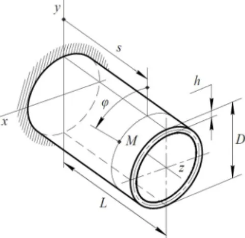
The shell is shown in Fig. 2. The left-hand edge of the shell is rigidly fixed, and the right-hand edge is free. In other words, the shell is supported like a cantilever with “clamped-free” boundary conditions. Thickness of the shell is regarded as be-ing much smaller than its diameter: ℎ ≪ = 2 . We will be using cylindrical coordinates: axial and angular . An arbitrary point belonging to the middle surface of the shell is said to have coordinates ( , ), as shown in Fig. 2.

Fig. 2 The shell’s dimensions and system of coordinates.

The shell is subjected to pin-load, which is represented by the two components of the cutting force: radial and circumferential , as shown in Fig. 1. We neglect the axial component of the cutting force because it is always much smaller than the other two components [4], and because the stiffness in the -direction is much higher than in the other two directions. Forces and act on the point with co-ordinates ( , 0). We introduce Λ as a changeable dimensionless parameter so that = Λ ⋅ , see (Fig. 1). We can now write down the expression for the shell's thickness:

ℎ( ) = ℎ if <

4

where ℎ is the shell's thickness before cutting and ℎ is the shell's thickness af-ter cutting.

According to [6], the general system of equations for a Kirchhoff-Love thin-walled cylindrical shell shown in Fig. 2 may be written [10] in matrix form

= (4)

where is a linear partial differential operator represented by (8 × 8) matrix and

= { , , , , , ∗_, ∗_{, } (5)}

is the state vector and

= − ⋅ {0, 0, 0, 0, , , , 0}. (6)

is the load vector. Here is the shell's radius, is the axial direction displace-ment, is the circumferential direction displacedisplace-ment, is the radial direction dis-placement, is the surface normal's angular displacement, , ∗, ∗, are the internal forces, and , , represent distributed external loading. Equation (4) represents a linear system of partial differential equations. It is possible to separate

and with the aid of the Fourier method using complex Fourier series:

= ∑ ( )exp( ). (7)

After separation of variables, system (4) is decomposed into the infinite amount of linear 8-th order systems of ordinary differential equations (ODE). Each of these ODE systems can be written in matrix notation as follows

( )= ( ) ( )+ ( ) (8)

( )= ⎣ ⎢ ⎢ ⎢ ⎢ ⎢ ⎢ ⎢ ⎢ ⎢ ⎢ ⎢ ⎡ 0 − − 0 0 0 0 − 0 0 0 0 ( ) 0 0 0 0 0 −1 0 0 0 0 0 − − 0 0 0 0 0 0 − 0 − 0 0 0 − 0 − 0 0 − 0 0 0 0 − 0 0 0 0 1 0 _⎦⎥ ⎥ ⎥ ⎥ ⎥ ⎥ ⎥ ⎥ ⎥ ⎥ ⎥ ⎤ (9)

where is the Young modulus, is the Poisson's ratio, ℎ is the shell's wall-thickness and

=

( ), = 1 + , = 1 + . (10)

Keeping in mind that dim ( ) = 1/dim( ), it is quite obvious that

{ , , } = {0, , − } ( ) ( ) . (11)

Using the Fourier series of the Dirac delta function

( ) = (2 ) ∑ exp( ) , (12)

the load vector can be rewritten as

( )= {0, 0, 0, 0, 0, − , , 0} ( − ). (13)

The left end of the shell ( = 0) is rigidly fixed, and the right end ( = ) is free. The followings are the boundary conditions:

{ , , , }_{( )}= 0 at = 0 { , ∗_, ∗_{, }}

( )= 0 at =

(14)

Here are the continuity conditions at point ( = ):

( )( + ) = ( )( − ) + {0, 0, 0, 0, 0, − , , 0} (15)

where is an infinitesimally small parameter. System (8) along with boundary conditions (14) represent a boundary value problem. We have used the initial

pa-6

rameters method [6] in order to solve this problem by means of numerical integra-tion. The Godunov orthogonalization method [7] was incorporated to ensure nu-merical stability of the solution. Moreover, the method was further modified in or-der to eliminate the well-known Gram-Schmidt process's weakness [8]. The Gram-Schmidt process was replaced by the Householder transformation [9], which effectively performs the same thing—orthonormalizes a set of vectors in the Euclidean space ℝ . Harmonic ( )( ) that corresponds to the radial

dis-placements of points located on the free end of the shell, can be represented as a linear combination of the cutting force components:

( )( ) = ⋅ ( )+ ⋅ ( ) (16)

where coefficients ( ) and ( ) depend only on parameter Λ and have been

ob-tained after numerical integration of the boundary value problem for different harmonics. According to expression (7),

( )( , ) = ∑ ( )+ ( ) exp( ) (17)

According to the definition (see Fig. 1), we can write that = ( , Φ ) and = ( , Φ ). Finally, according to formulas (1) and (2), matrix can be repre-sented as an infinite series

= ∑ ( )exp( Φ ) ( )exp( Φ )

( )exp(− Φ ) ( )exp(− Φ )

. (18)

It can be shown that the components of matrix are always real numbers, which they must be, of course, since is the flexibility matrix. The criteria of meeting the required accuracy has been

‖ − ‖ ⋅ ‖ ‖ ≤ . (19)

If the above inequality is satisfied, then we consider approximation to be accu-rate enough. In our work, we have set the relative accuracy to = 0.01 = 1%. The magnitude of the cutting force is approximately 10 –10 N, according to [4]. Using this data and our model, we have calculated that magnitudes of the dis-placements are within 10 m.

The components of matrix are dependent on the three variable parameters that we have introduced earlier: = (Φ , Φ , Λ).

3.0 Optimization of the Displacement Sensors Location

We need to determine the best set of parameters Φ and Φ (the displacement sen-sors angular location) that would make the system (1) as well-conditioned as pos-sible. Measure of a square matrix's numerical stability is called its condition num-ber . By definition [8],

( ) = ‖ ‖ ⋅ ‖ ‖ . (20)

Condition number is always positive and cannot be less than one. The closer the condition number of the flexibility matrix is to one, the better conditioned this matrix is. Therefore, to ensure the best numerical stability of the linear transfor-mation (1) we must minimize the condition number of matrix . Let us con-struct the target function

(Φ , Φ ) = max (Φ , Φ , Λ) . (21)

To accomplish our optimization goal we have had to minimize :

→ min, Φ , Φ = arg min ∈[ , ]& ∈[ , ] (Φ , Φ ) . (22)

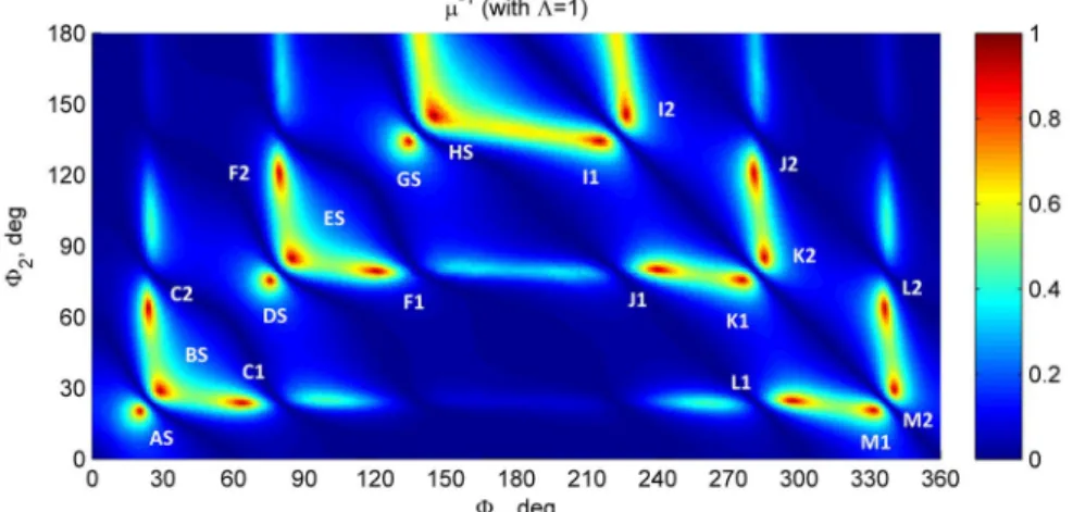
We have implemented the brute force approach minimizing function . Angular increment has been set to 0.1°, and the increment for parameter Λ has been set to 0.05. Color plot of function (Φ , Φ , 1) is shown in Fig. 4. We have cho-sen to analyze function inverse to the condition number because this function is normalized: its range of values lies inside interval (0, 1). The diagram reveals 20

local maxima of (see Fig. 4 and Table 1). The best choice of parameters (i.e. the

global maxima) turned out to be Φ = Φ = 20.4°, which corresponds to the

target function value of 1.2. This displacement sensors’ configuration is shown in Fig. 3.

Fig. 3 Optimal displacement sensors location.

Strictly speaking, this value is the global minimum of function (Φ , Φ ). How-ever, in practical terms, any of the displacement sensors configurations from Table 1 can be chosen because magnitude of for any of those configurations does not even exceed the value of 10. It means that at the worst case scenario we could lose 1–2 significant digits [8] calculating the components of the cutting force using

8

equation (1), which corresponds to relative accuracy = 10 . Such loss is not significant in comparison with other sources of error in our model.

Fig. 4 Optimal displacement sensors’ angular location configurations. Table. 1 Optimal displacement sensors angular location configurations.

# Φ Φ ‖ ‖ ⋅ 10 # Φ Φ ‖ ‖ ⋅ 10 AS 20.4 20.4 1.2 8.2 I1 208.3 137.5 1.8 0.59 BS 30.6 30.6 1.5 7.2 I2 222.5 151.7 1.8 0.59 C1 66.6 24.3 1.5 9.7 J1 241.1 83.5 2.0 2.1 C2 24.3 66.6 1.5 9.7 J2 276.5 119.9 2.0 2.1 DS 77.7 77.7 2.8 3.8 K1 268.5 78.6 2.0 2.7 ES 89.3 89.3 1.9 1.6 K2 281.5 91.5 2.0 2.7 F1 119.4 83.5 1.4 2.2 L1 293.5 25.3 1.4 7.1 F2 83.5 119.4 1.4 2.2 L2 334.7 66.5 1.4 7.1 GS 136.2 136.2 1.4 0.87 M1 329.3 20.5 1.2 7.6 HS 149.5 149.5 1.7 0.37 M2 339.5 30.7 1.2 7.6

Index ‘S’ in Table 1 represents -symmetrical configurations, and indexes ‘1’ and ‘2’ represent identical configurations. Table 1 also features minimum value of norm of matrix , which represents magnitude of displacements of measured points. Note that

dim = dim‖ ‖ = mm N⁄ . (23)

We can see that configurations GS, HS, I1 and I2 are probably not preferable be-cause the displacements would be significantly smaller than in the other configu-rations. From this point of view, configurations AS, BS, C1, C2, L1, L2, M1, M2 are optimal, and each of them can be readily picked by an experimenter.

4.0 Conclusion

In this work we have developed a mathematical model in order to be able to calculate the flexibility matrix that makes it possible to estimate the cutting force components based on displacement measurement in turning cylindrical shells. Analysis of the behavior of the flexibility matrix condition number has been performed. Based on this analysis, optimal configurations of the displacement sensors location have been suggested. These configurations make the flexibility matrix well-conditioned and the process of calculating the components of the cutting force numerically stable. Any of these configurations can be picked as they do not cause numerical instabilities when calculating the flexibility matrix.

References

[1] Fang N., Q. Wu. A Comparative Study of the Cutting Forces in High Speed Machining of Ti-6Al-4V and Inconel 718 with a Round Cutting Edge Tool. Journal of Materials Processing Technology. 2009. Vol. 209 (9). Pp. 4385–4389.

[2] Sun S., Brandt M., Dargusch M.S. Characteristics of cutting forces and chip formation in ma-chining of titanium alloys. International Journal of Machine Tools and Manufacture. Vol. 49 (7–8). Pp. 561–568.

[3] Kim Tae-Yong, Kim Jongwon. Adaptive cutting force control for a machining center by using indirect cutting force measurements. International Journal of Machine Tools and Ma-nufacture. Vol. 36 (8). Pp. 925–937.

[4] Lorong P., Larue A., and Duarte A. P. Dynamic Study of Thin Wall Part Turning. Advanced Materials Research. 2011. Vol. 223. Pp. 591–599. DOI: 10.4028.

[5] Gerasimenko A. A., Gouskov A. M., Guskov M. A., Lorong P. Spinning shell eigen modes calculation. Vestnik MGTU imeni Baumana, 2012.

[6] Biderman, V. L. Mekhanika tonkostennykh konstruktsiy. Moscow, 1997. [7] Godunov, S. K. 1961 On the numerical solution of boundary value problems for

systems of linear ordinary differential equations. Uspehi. Mat. Nauk. 16, 171–174. [8] Higham N. J. Accuracy and Stability of Numerical Algorithms. 2nd ed. Philadelphia:

SIAM. 2002.

[9] Householder A. S. Unitary Triangularization of a Nonsymmetric Matrix. Journal of the ACM. 1958. Vol. 5 (4). Pp. 339–342. DOI:10.1145/320941.320947.

[10] Kondratenko K. E., Gouskov A. M., Guskov M. A., Lorong. P., Panovko G. Ya. Analysis of indirect measurement of cutting forces in turning metal cylindrical shells. Vestnik MGTU imeni Baumana, 2014. DOI: 10.7463/0214.0687971.