doi: 10.3389/fenvs.2018.00025
Edited by: Philippe C. Baveye, AgroParisTech Institut des Sciences et Industries du Vivant et de L’environnement, France Reviewed by: Andrey S. Zaitsev, Justus Liebig Universität Gießen, Germany Klaus Lorenz, The Ohio State University, United States *Correspondence: Simon Tresch tresch.simon@gmail.com
Specialty section: This article was submitted to Soil Processes, a section of the journal Frontiers in Environmental Science Received: 08 February 2018 Accepted: 18 April 2018 Published: 08 May 2018 Citation: Tresch S, Moretti M, Le Bayon R-C, Mäder P, Zanetta A, Frey D and Fliessbach A (2018) A Gardener’s Influence on Urban Soil Quality. Front. Environ. Sci. 6:25. doi: 10.3389/fenvs.2018.00025
A Gardener’s Influence on Urban Soil
Quality
Simon Tresch1,2,3*, Marco Moretti3, Renée-Claire Le Bayon1, Paul Mäder2,
Andrea Zanetta3,4, David Frey3,5and Andreas Fliessbach2
1Functional Ecology Laboratory, Institute of Biology, University of Neuchâtel, Neuchâtel, Switzerland,2Department of Soil
Sciences, Research Institute of Organic Agriculture (FiBL), Frick, Switzerland,3Biodiversity and Conservation Biology, Swiss
Federal Research Institute WSL, Birmensdorf, Switzerland,4Department of Biology, Ecology & Evolution, University of
Fribourg, Fribourg, Switzerland,5Department of Environmental System Science, Institute of Terrestrial Ecosystems, ETH
Zurich, Zurich, Switzerland
Gardens are hot spots for urban biodiversity and provide habitats for many plant and animal species, both above- and below-ground. Furthermore, gardens provide a wide range of ecosystem services, including carbon (C) storage and nutrient cycling. Although the soil is the foundation of sustainable gardens providing those ecosystem services, very little is known about the consequences of garden management on soil quality. Here we present a comprehensive assessment of urban garden soil quality, including biotic and abiotic site characteristics combined with land-use history and garden management information in a multivariate evaluation. A set of 44 soil quality indicators was measured at 170 sites of 85 gardens in the city of Zurich, Switzerland, comprising contrastingly managed garden habitats along a gradient of urban density. Taken together, our results show that garden management was the driving factor that influenced soil quality and soil functions. Eco-physiological soil quality indices were useful to identify differences in disturbance and intensity of soil use, showing highest microbial [microbial biomass (Cmic)/soil organic carbon (SOC)] and lowest metabolic (qCO2) quotients in perennial
grass sites compared to annual vegetable sites. Despite the intensity of soil disturbance in annual vegetable and flower beds, the highest endogeic earthworm biomass and diversity were found in those habitats. Whereas decomposition of green tea bags was higher in grass sites. Soil heavy metal contents varied considerably and could not be linked with garden management practices, but with spatial patterns of industry and traffic. We conclude that understanding soil quality in urban ecosystems needs multi-indicator frameworks to capture the complexity of soil characteristics and the influencing factors in space and time. This study contributes to a better understanding of urban gardens and enhances the development of sustainable soil management strategies aimed at long-term improvement of soil quality and related ecosystem services in cities.
Keywords: urban gardening, soil quality indicators, Cmic/SOC, qCO2, urban ecology theory, urban ecosystem services, earthworms, tea bag index
1. INTRODUCTION
Urban gardens are hot spots of urban biodiversity, serving as fertile islands for plants and animals in increasingly densified cities (e.g., Gilbert, 1989; Owen, 2010). Besides their importance as ecological niches for many species (Smith et al., 2006), they increase the connectivity of urban landscapes (Rudd et al., 2002) and provide multiple ecosystem services (Elmqvist et al., 2015). Urban gardens give the opportunity for people, particularly children (Hand et al., 2017), to interact with nature (Miller, 2005). Soil is the foundation of urban habitats that provide key ecosystem services in cities (Zhu et al., 2018). Urban garden soils are important for regulating the micro-climate by providing shade and allowing water to infiltrate and evaporate (Bowler et al., 2010). Moreover, they improve air quality (Janhäll, 2015), prevent flooding by reducing surface-water run-off (Bolund and Hunhammar, 1999), storing a considerable amount of soil organic carbon (SOC) (Edmondson et al., 2012) and improve pollination by hosting diverse insect species (Samnegård et al., 2011). But in many cities the sealed area is expanding tremendously with negative consequences for these ecosystem services (Sachs, 2015), especially for contested urban green spaces like allotment gardens (Tappert et al., 2018), due to the need for accommodation and infrastructure of growing urban populations.
Urban soils are often associated with degraded and possibly polluted soils (Meuser, 2010), low in SOC (e.g., Craul, 1999; Bradley et al., 2005) and biological activity (e.g., Lorenz and Kandeler, 2005; Scharenbroch et al., 2005), compared to non-urban soils in forests or croplands. Urban soil properties may be altered by anthropogenic disturbances such as compaction due to construction activities or various soil management practices such as fertilization, mowing, or drainage (Lorenz, 2017). For this reason disturbed urban soils were generally considered to have a low physical and chemical quality, not suitable for crop production (Jim, 1998). More recently urban soils are looked at from a different angle with the increasing interest in urban agriculture. Urban garden soils can be fertile and can support soil functions despite intensive soil use (Levin et al., 2017). For instance, Edmondson et al. (2014) and Vasenev et al. (2013)
found increased SOC values in urban gardens compared to non-urban soils.
Soil quality can be defined as “the capacity of a soil to function within ecosystem and land-use boundaries, to sustain biological productivity, maintain environmental quality, and promote plant and animal health,” including human health (Doran and Parkin, 1994). This comprehensive but complex definition refers to the multi-functionality of soils providing ecosystem services but also to the site specificity of the soil properties (Bünemann et al., 2018). Urban gardens not only provide vegetables and fruits, they are also important to conserve and provide niches for above- and below-ground biodiversity. A definition of soil fertility is given in the Swiss ordinance on impacts on soils (Swiss Federal Council, 1998) comprising among others the ability of harboring a biologically active community, a typical site-specific soil structure, an undisturbed decomposition and no risk for
humans and animals, when they take it up directly. We evaluated soil quality using a comprehensive set of inherent and dynamic soil properties, which were often used in soil quality assessment approaches (Bünemann et al., 2018). In addition to 44 measures of soil quality (MSQ), we analyzed the decomposability of tea bags and the suitability of habitats for earthworms as important soil functions. Moreover, the distribution and contents of heavy metals have been evaluated, since they are a major concern in urban soils (Kim et al., 2014). Earthworms are sensitive to both soil management (Pulleman et al., 2012) and soil pollution (Pérès et al., 2011) and functional groups of earthworms have distinct impact on soil functions such as soil structure and decomposition (Edwards, 2004). Only few studies have investigated soil quality or soil functions in urban gardens (Beniston et al., 2016), which is probably because of the difficulties associated with gaining access to private properties (Goddard et al., 2010). Findings that gardening activities, such as regular clearing, digging, planting, weeding, and watering the soil, can have a significant impact on above-ground biodiversity (Smith et al., 2006; Goddard et al., 2013), suggest that garden management will also affect the quality of urban garden soils. However, little is known how these management practices affect below-ground diversity and soil quality (e.g.,Edmondson et al., 2014; Amossé et al., 2016).
In relation to the central principle in urban ecology theory, that anthropogenic management controls ecosystem processes (e.g., Alberti, 1999), we determined the impact of gardening practices on soil properties and soil functions. A multivariate approach combining management and garden characteristics with a comprehensive set of MSQ (Table 1) was conducted on a city wide sampling approach including the two most common urban garden types (allotment and home gardens). Effects of soil disturbance were further studied by the use of eco-physiological soil indices introduced byAnderson and Domsch (1989), who used them to show the influence of management intensity on soil microbial communities. The authors found increased values for the metabolic quotient (qCO2) and decreased
for the microbial quotient (microbial biomass C (Cmic)/SOC) in
soils of monocropping systems compared to those under crop rotation. In this paper, we investigate the following four research hypothesis:
1. Garden management practices influence soil properties. 2. Biological soil quality measures, which are highly sensitive
to management in agricultural soils (Mäder et al., 2002), are strongly affected by garden management practices.
3. Sites with more frequent soil disturbance have a lower microbial (Cmic/SOC) and a higher metabolic (qCO2)
quotient.
4. Heavy metal contents have a negative impact on decomposition and earthworm abundance.
This study was part of an interdisciplinary project (www. bettergardens.ch) that focuses on the importance of urban gardens for biodiversity, ecosystem services, and human well-being. Our aim was to contribute to a key question in urban ecology (McPhearson et al., 2016): What is the impact of disturbance on soil functions? We propose an adapted multivariate method for assessing soil quality, which is urgently
needed to better understand the conditions of urban soils and the ecosystem services they provide (Zornoza et al., 2015).
2. MATERIALS AND METHODS
2.1. Study Sites and Design
The study took place in the city of Zurich (Switzerland; 47◦22′0′′N, 8◦33′0′′E), which is an average size European city
with approximately 0.4 million inhabitants. Zurich is located in the temperate climate zone with mean annual temperature of 9.3°C (1981–2010) and mean annual rainfall of 1,134 mm (MeteoSchweiz, 2017). The total area of Zurich is approximately 8,800 ha with 47% settlement area including buildings and gardens, 26% forest, 15% roads, 10% agriculture, and 2% water bodies (Statistical office Zurich, 2017). Allotment gardens, a plot of land rented by citizens interested in gardening, have been installed in Zurich since the beginning of the twentieth century and follow a long history of self-supplying citizen gardens, which goes back to the sixteenth century (Christl et al., 2004). The 5,500 allotment gardens cover 3% of total settlement area and 3% of urban green space in the city of Zurich, while home gardens, which are located around a private house, cover 11% of total settlement area and 25% of urban green space (Grün Stadt Zurich, 2010). The city wide soil quality assessment was done on 85 urban gardens (42 allotment and 43 home gardens), which were selected following a systematic nested design (Fortin et al., 1989). Allotment and home gardens were selected across two independent gradients: An urbanization density gradient and a gradient of garden management. The urbanization density gradient was assessed by the geographical position and the information about the built and sealed surface area around a garden. The gradient of garden management was visually assessed on-site by a professional gardener, ranging from intensively managed gardens consisting of vegetable plots to very natural gardens with flower meadows. Nested in each garden two study sites were selected to account for varying management concepts within a garden and to test for the effect of similar parental soil conditions. We focused on medium sized gardens with an average size of 312 ± 154 m2, to have a similar garden area in allotment and home gardens and because these small gardens account for the largest share of the total garden area in European cities (Loram et al., 2007). Gardens were first selected by aerial photographs (ArcGIS) and secondly by visual on-site inspection, before asking each garden owner for permission. Given the spatial and temporal complexity of urban environments we decided to focus on one city in order to consider all possible spatial components affecting urban soil quality in gardens and increase the statistical power of the nested design.
2.2. Soil Samples
Soil samples were taken from two distinct sites within each garden. One site was chosen in a more frequently disturbed garden area, usually cultivated with annual plants (e.g., vegetables) and the other in an area with less soil disturbance, such as sites covered with perennial vegetation (e.g., lawn). Sampling under the canopy of trees was avoided to minimize
undesirable confounding effects on soil properties. Soil samples were taken in March 2015 before the beginning of the gardening season (i.e., before major soil disturbances such as tillage, fertilization or planting). At each of the 170 sites, within an area 2 × 2 m, five soil samples were taken randomly from the 0 to 20 cm soil layer with a 30 mm wide soil auger. The soil samples were pooled per site and on arrival to the laboratory they were gently air dried prior to homogenization with an analytical sieve (2 mm mesh size), removing visible roots, other plant material and stones. The samples were stored at 4°C until further analysis. For the soil physical measurements, three soil cores (5 cm diameter & depth, Eijkelkamp, NL) were taken at a depth of 10–15 cm at each site.
2.3. Measures of Soil Quality (MSQ)
A total of 44 measurements were obtained on all 170 sites (Table 1), according to Swiss standard methods for physical, chemical, and biological soil characterization (Agroscope, 2012), if not stated otherwise. Soil water content was determined gravimetrically, after drying soil at 105°C for 24 h. The pH and electrical conductivity (EC) of air dried sub samples were measured in a soil suspension with deionized water (1:2.5, w/v). The maximum soil water holding capacity (WHC) was determined by a cylinder method, where field moist soil is saturated with water on a sand bath (Schinner et al., 1996). Soil aggregate stability (SA) was measured as the proportion of stable aggregates (1–2 mm) left after 5 min. of wet sieving on a multi-sieve device with a frequency of 42 cycles min−1
subtracting the sand fraction (Schinner et al., 1996). Particle size distribution for clay, silt, and sand contents was measured by a combined sieving and sedimentation technique, while soil texture was classified according to USDA taxonomy. Pore space volume and soil bulk density (BD) were determined with the undisturbed soil cores, where latter was determined as the soil mass dried at 105°C related to the total volume of the cylinders. Penetration resistance was measured using a Penetrologger (Eijkelkamp, NL) with a cone type of 10−4 m2 and a penetration speed of 0.02 m s−1 down to a maximum
soil depth of 80 cm, recording the penetration resistance every 1 cm. Ten replicate measurements were taken for each 2 × 2 m area and mean values for penetration resistance were taken from 0–20 cm. Soil nutrient contents (P, K, Mg, Cu, Fe, Mn, B) were measured externally at a certified laboratory with ammonium acetate-EDTA. SOC and total organic nitrogen (TON) were analyzed by a CHN analyser (Thermo Scientific Flash EA 1112, NL) after removing carbonates by acidifying the soil with HCl (2 M). Dissolved organic carbon (DOC), dissolved organic nitrogen (DON), and mineral nitrogen (Nmin)
were measured in an extract with 0.01 M CaCl2 (1:4, w/v).
Mineral nitrogen (Nmin) (nitrate and ammonium) was analyzed
spectrometrically (SAN-plus Segmented Flow Analyser, Skalar Analytical, NL) and DOC and DON with a TOC/TNb analyser (multi N/C 2100 S, Analytic Jena AG, D) described inKrauss et al. (2017). Soil biological analyses were conducted at 40– 50% maximum WHC. Soil microbial biomass carbon (Cmic)
and nitrogen (Nmic) contents were estimated by
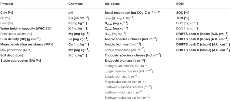
TABLE 1 | Measures of soil quality (MSQ) (N = 44) obtained in all urban garden sites (N = 170).
Physical Chemical Biological SOM
Clay [%] pH Basal respiration [µg CO2-C g−1h−1] SOC [%]
Silt [%] EC [µS cm−1] Cmin[g CO2-C kg−1] TON [%]
Sand [%] P [mg kg−1] Nmin[mg kg−1] DOC [mg kg−1]
Water holding capacity (WHC) [%] K [mg kg−1] Cmic[mg kg−1] DON [mg kg−1]
Pore space volume [%] Mg [mg kg−1] Nmic[mg kg−1] DRIFTS peak A (labile) [A.U. cm−1]
Bulk density (BD) [g cm−3] Fe [mg kg−1] Anecic species richness [ind. m−2] DRIFTS peak B (labile) [A.U. cm−1] Mean penetration resistance [MPa] Cu [mg kg−1] Anecic biomass [g m−2] DRIFTS peak C (stable) [A.U. cm−1]
Max penetration [MPa] Mn [mg kg−1] Anecic abundance [ind. m−2] DRIFTS peak D (stable) [A.U. cm−1]
Soil depth [cm] B [mg kg−1] Endogeic species richness [ind. m−2]
Stable aggregates (SA) [%] Endogeic biomass [g m−2]
Endogeic abundance [ind. m−2] Epigeic species richness [ind. m−2] Epigeic biomass [g m−2] Epigeic abundance [ind. m−2] Earthworm species richness [m−2] Earthworm biomass [g m−2] Earthworm abundance [ind. m−2]
Bold printed measurements (N = 28) were used for the soil quality assessment after excluding variables with r > 0.6 and/or a variable inflation factor > 4 (Borcard et al., 2011).
with triplicates of 20 g soil subsamples followingFliessbach et al. (2007). Soil respiration was measured with 30 g of soil on a gas chromatograph (7890A, Agilent Technologies, USA) equipped with a thermal conductivity detector (TCD; details are provided in Table S12). Basal respiration (resp) rates were recorded after 1 week and C mineralization (Cmin) as cumulative values after 4
weeks of soil incubation at 20°C.
2.3.1. Soil Organic Matter Characterization
Soil organic matter (SOM) was characterized using diffuse reflectance Fourier transform mid-infrared spectroscopy (DRIFTS) following Rasche et al. (2013). Measurement details are given in Table S13. Out of 19 calculated DRIFTS peaks two labile peaks (A & B) and two stable peaks (C & D) of organic functional groups were inspected in detail by consulting the DRIFTS fingerprint database and the literature on stable or labile SOM compounds. Peak A ranging from 1,080 to 950 cm−1, was characterized as a labile compound of SOM
linked to polysaccharide-C (Lehmann et al., 2007). Peak B (1,148–1,170 cm−1) was linked to labile poly-alcoholic and
ether functional groups (Spaccini and Piccolo, 2007; Demyan et al., 2012). Peak C (1,660–1,580 cm−1) was associated with aromatic compounds (Baes and Bloom, 1989; Demyan et al., 2012) representing stable functional compounds of SOM. Peak D (3,010–2,800 cm−1) was related to aliphatic
compounds (Baes and Bloom, 1989; Lehmann et al., 2007), representing a relatively labile SOM fraction (Mirzaeitalarposhti et al., 2016), although it can also be correlated with SOC contents (Gerzabek et al., 2006) due to carbonate interference (Mirzaeitalarposhti et al., 2016) and is therefore suspected to represent rather stable functional organic groups of SOM in this study.
2.4. Explanatory Variables
2.4.1. Garden Management
A survey including all gardeners was carried out to collect information on garden management and gardener’s intentions (see Table 2). An ethics approval was not required for this research according to institutional and national guidelines. The consent of the participants was obtained by virtue of survey completion. Relevant soil management questions were asked individually for each of the five common garden habitat types (lawn, meadow, vegetable bed, flower bed, and berry cultivation). These habitat types were later grouped into three categories according to the degree of associated soil disturbance: annual vegetation (vegetables), perennial vegetation with herbaceous vegetation (berries and perennial flowers), and grass vegetation (meadows and lawn).
2.4.2. Garden Characteristics
Garden characteristics (Table 2) were measured at the sampling site level within each garden. The variables “former land-use” and “history” were assessed using digital historic maps (1864– 2016) from Swiss Federal Office of Topography (2017). The urbanization density was measured as a percentage of the sealed and built area around each garden with five radii (30, 50, 100, 250, 500 m) obtained in ArcGIS. In order to reduce the complexity of response variables, these sealed areas on five scales were replaced with a measure of the urban heat island (UHI), which was highly correlated with those variables (r = 0.7–0.8; Figure S10). In general, the UHI effect refers to the warmer temperatures within a city compared to rural areas. We used the local deviation of mean night temperatures near the surface (0 to + 6 K) from a regional climate model of Parlow et al. (2010). This UHI effect will be referred as the urbanization density gradient (“overwarming”; Figure 1 and Figure S1) in this study.
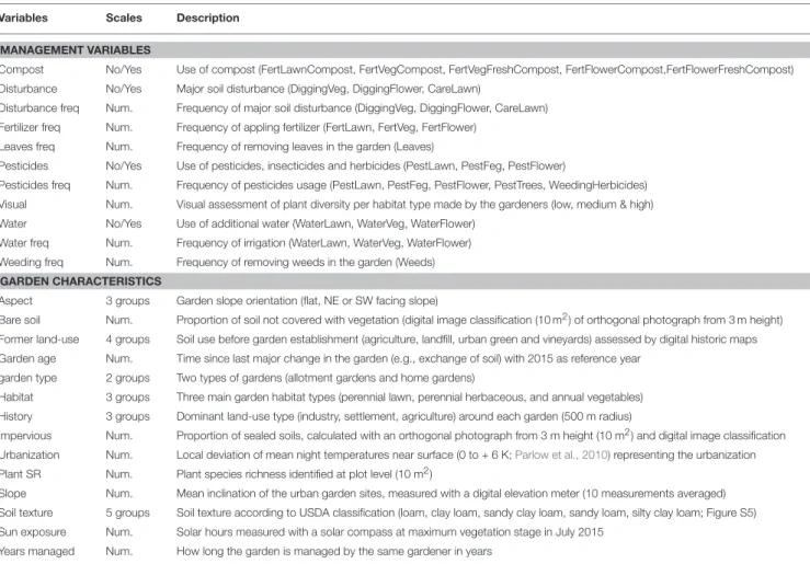
TABLE 2 | Response variables potentially influencing soil quality of urban gardens.
Variables Scales Description
MANAGEMENT VARIABLES
Compost No/Yes Use of compost (FertLawnCompost, FertVegCompost, FertVegFreshCompost, FertFlowerCompost,FertFlowerFreshCompost) Disturbance No/Yes Major soil disturbance (DiggingVeg, DiggingFlower, CareLawn)
Disturbance freq Num. Frequency of major soil disturbance (DiggingVeg, DiggingFlower, CareLawn) Fertilizer freq Num. Frequency of appling fertilizer (FertLawn, FertVeg, FertFlower)
Leaves freq Num. Frequency of removing leaves in the garden (Leaves)
Pesticides No/Yes Use of pesticides, insecticides and herbicides (PestLawn, PestFeg, PestFlower)
Pesticides freq Num. Frequency of pesticides usage (PestLawn, PestFeg, PestFlower, PestTrees, WeedingHerbicides) Visual Num. Visual assessment of plant diversity per habitat type made by the gardeners (low, medium & high) Water No/Yes Use of additional water (WaterLawn, WaterVeg, WaterFlower)
Water freq Num. Frequency of irrigation (WaterLawn, WaterVeg, WaterFlower) Weeding freq Num. Frequency of removing weeds in the garden (Weeds)
GARDEN CHARACTERISTICS
Aspect 3 groups Garden slope orientation (flat, NE or SW facing slope)
Bare soil Num. Proportion of soil not covered with vegetation (digital image classification (10 m2) of orthogonal photograph from 3 m height) Former land-use 4 groups Soil use before garden establishment (agriculture, landfill, urban green and vineyards) assessed by digital historic maps Garden age Num. Time since last major change in the garden (e.g., exchange of soil) with 2015 as reference year
garden type 2 groups Two types of gardens (allotment gardens and home gardens)
Habitat 3 groups Three main garden habitat types (perennial lawn, perennial herbaceous, and annual vegetables) History 3 groups Dominant land-use type (industry, settlement, agriculture) around each garden (500 m radius)
Impervious Num. Proportion of sealed soils, calculated with an orthogonal photograph from 3 m height (10 m2) and digital image classification Urbanization Num. Local deviation of mean night temperatures near surface (0 to + 6 K;Parlow et al., 2010) representing the urbanization Plant SR Num. Plant species richness identified at plot level (10 m2)
Slope Num. Mean inclination of the urban garden sites, measured with a digital elevation meter (10 measurements averaged) Soil texture 5 groups Soil texture according to USDA classification (loam, clay loam, sandy clay loam, sandy loam, silty clay loam; Figure S5) Sun exposure Num. Solar hours measured with a solar compass at maximum vegetation stage in July 2015
Years managed Num. How long the garden is managed by the same gardener in years
Corresponding questions asked in gardener survey are in brackets. Most management questions were asked on a five level Likert scale and normalized by the total number of questions for the combined management variables. Survey questions are described in Table S10.
2.4.3. Spatial Structure
To account for spatial autocorrelation of the MSQ (Figure 2) we used Moran Eigenvector Maps (MEM) following the instructions of Borcard et al. (2011). The MEM method decomposes the eigenvalues, which represent spatial relationships of the geographic connectivity matrix, into eigenvectors addressing significant spatial variation at various scales (Braaker et al., 2014). The MEM reflect correlations of the MSQ between and within the gardens and can therefore be used in the models to address for unaccounted variation due to spatial autocorrelation not covered by other variables (Figure S3). Delaunay triangulation was chosen as an optimal spatial matrix, representing the connections of the urban gardens. Model selection was performed according to the lowest Akaike information criterion with small sample size correction (AICc), resulting in 19 significant MEM.
2.4.4. Soil Heavy Metals
Total element concentrations of heavy metals (As, Ba, Co, Cr, Cu, Cd, Ni, Pb, Sb, V, Zn) were analyzed using dried and ball milled soil samples pressed with wax to tablets using a Spectro X-lab 2000 X-Ray Fluorescence (XRF)
spectrometer. This technique conforms with standard measurements of soil heavy metal concentrations (Horta et al., 2015), except for Cd (Christl et al., 2004), which were excluded.
2.5. Soil Functions
2.5.1. Habitat for Earthworms
The suitability of habitat for soil fauna was investigated by the abundance, biomass and species richness of functional groups of earthworms. They were collected in September and October 2015 using a combined mustard (0.6%) extraction (Lawrence and Bowers, 2002) and hand sorting method (Bartlett et al., 2010). The animals were collected from an area of 0.3 × 0.3 m within the same 2 × 2 m areas used for the soil samples and stored in 70% ethanol for species identification (Bouché, 1977; Sims and Gerard, 1999; Blakemore, 2008). The species were classified according to three ecological groups with respect to their main vertical distribution in the soil (epigeic, endogeic, and anecic) as defined by Bouché (1977). Juveniles could only be assigned to ecological categories and were used for the total earthworm biomass and abundance calculation.
FIGURE 1 | (A) Urban gardens analyzed in the city of Zurich (85 urban gardens with two sampling sites per garden). Colors correspond to the garden types (blue: allotment, red: home) and the point size to the urbanization density gradient, which is represented by a regional climate model with local deviation of mean night temperatures near surface from 0 to + 6 K (Parlow et al., 2010). (B) Values of local mean night temperature deviations (overwarming), representing the urbanization density gradient in this study.
FIGURE 2 | Scheme for the multivariate soil quality assessment. (A) There are in total 44 measures of soil quality (MSQ). Exclusion criteria (r < 0.6 and or a variance inflation factor >4 (Borcard et al., 2011)) reduced MSQ by 16 variables. (B) Explanatory variables are written in italics. Moran eigenvector maps (MEM) were selected based on smallest AICc (cf. section 2.4.3). (C) MSQ as response matrix with Euclidean distances and explanatory variables (Figure S11) were used in a PERMANOVA. Thereafter, significant explanatory variables (p <0.05) were fitted on the NMDS ordination of MSQ. A fuzzy clustering of the MSQ was obtained and the three groups were plotted on the NMDS plot (Figure 3).
2.5.2. Decomposition Rates of Tea Bags
Decomposition was assessed by using standardized commercial tea bags buried in the soil, following the tea bag index (TBI) protocol byKeuskamp et al. (2013). Decomposition was mainly done by microorganisms, due to the small mesh size of the nylon
bags (Setälä et al., 1996). Two types of litter decomposition were assessed by using rooibos tea as a slowly decomposable and green tea as a fast decomposable organic material. We buried four tea bags per tea type, resulting in 1,360 buried tea bags (85 gardens × 2 sites × 2 different tea types × 4 replicates), for 90
days (mid-October 2015 until mid-January 2016) at a depth of 8 cm. Teabags were weighed after drying at 60°C, before and after the incubation in the field. Additionally to the TBI protocol, soil particles, which entered the tea bags were subtracted after incineration of the bags.
2.6. Soil Quality Indices
Three indices of soil quality were calculated from the MSQ. The ratio of SOC to clay was calculated as an indicator of structural soil quality (Johannes et al., 2017). Further eco-physiological indices of soil quality were calculated using the ratio of Cmic
to SOC (microbial quotient) as an indicator of SOM quality for microbes and the metabolic quotient (qCO2) calculated as
the ratio of basal respiration rate to Cmic, which describes the
substrate mineralized per unit of microbial biomass carbon (Anderson, 2003).
2.7. Multivariate Soil Quality Assessment
After variable selection (Figure 2) a fuzzy cluster analysis was performed as a multivariate technique to group garden sites with similar MSQ. Prior to the clustering, data was normalized and a Euclidean distance matrix was calculated, as it was the most appropriate distance matrix according to its rank correlations (Oksanen, 2011). A non-metric multidimensional scaling (NMDS) was applied to visualize the cluster groups and to draw inference about the response variables. NMDS produces a rank-based ordination on a distance or dissimilarity matrix and is regarded as the most robust unconstrained ordination method (Minchin, 1987), because it tolerates quantitative, semi-quantitative, qualitative, or mixed variables (Borcard et al.,
2011). A similar approach has been applied to group soils of different land-use types according to the soil quality in Italy (Marzaioli et al., 2010). Permutational multivariate analysis of variance (PERMANOVA) was performed with the MSQ as Euclidean distance response matrix and significant variables (p ≤ 0.05) were fitted to the NMDS ordination, while MEM variables were excluded to increase visibility of the main effects. Due to the influence of the habitat types in the PERMANOVA (Table S2), a second NMDS analysis per habitat types (NMDS habitat) was conducted for the garden management questions (Figure S4, Table S4). Correlations were analyzed by Pearson correlation coefficients (r). Linear mixed effect models (LMEM) were fitted after analysing the model assumptions (independent and identical distributed residuals). Fixed effects were garden habitat types (3 factors), garden types (2 factors), and the urbanization density, while the garden identity was set as a random factor. Means and 95% credible intervals of the Bayesian inference posterior distributions were calculated following
Korner-Nievergelt et al. (2015). All statistical analyses were performed using R 3.3.1 (R Core Team, 2017). A detailed description of each function and the corresponding R packages is given in Table S14.
3. RESULTS
3.1. Urban Soil Quality Assessment
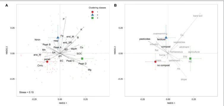
Garden sites were grouped into three main clusters (fuzzy clustering). With the NMDS ordination (Figure 3) we could show that the first cluster (red dot) contained home garden sites, dominated by grass sites with high content of Cmic,
FIGURE 3 | (A) Multivariate NMDS ordination of significant (PERMANOVA, Table S1) measures of soil quality (MSQ). Colors and symbols correspond to different groups of soil quality based on a fuzzy clustering. (B) Biplot of management (black) and garden characteristics (gray) fitted on the NMDS ordination of plot (A). Only significant variables from PERMANOVA p ≤ 0.05 are displayed in (B), while MEM were excluded. ane_M, anecic biomass; end_M, endogeic biomass; end_SR, endogeic species richness; resp, basal respiration; penet, penetration resistance; BD, bulk density; SA, stable aggregates.
penetration resistance, and anecic earthworms biomass and species richness. The second cluster (blue triangle) included vegetables sites and allotment gardens, which have much “bare soil” and are surrounded by “industry” and are located within the more densified urban areas (“overwarming”). This group had high contents of basal respiration, Nmin, nutrients (Fe, P,
K, B), labile SOM compounds (Peak A & B), and endogeic earthworms biomass and species richness. The third cluster (green square) was characterized by herbaceous sites surrounded by “agriculture” and consisting of a “slope” (either facing NE or SW) with high contents of Mg, SOC, Cu (as micro-nutrient), As, aliphatic and aromatic SOM compounds (Peak C & D). The most important variables for the NMDS ordination (p ≤0.001, Table S1) were chemical (Mg, P, Fe, K, pH, Mn, B, and Mn), biological (Cmic, resp, and Nmin), physical (SA, penetration resistance and
BD) as well as SOM (Peaks A, B, C, D, and SOC) measurements.
3.2. Effects of Garden Management
The frequency of using pesticides (PERMANOVA; F = 6.4, P <0.001) and fertilizers (PERMANOVA; F = 2.4, P = 0.05) as well as the use of compost (PERMANOVA; F = 6, P < 0.001) indicated the biggest effects of management variables on the NMDS ordination (Table S2). For perennial grass sites the date of the first lawn mowing in a year, was the only siginficant management variable (NMDS habitat; P = 0.04, Table S4). If the first cut was earlier, P (r = −0.26, P = 0.04) and Fe contents (r = −0.29, P = 0.02) were higher, but BD (r = 0.28, P = 0.03; Table S3) was lower. For the sites under perennial herbaceous vegetation, the use of relatively young compost, less than 1 year old (“FertFlowerFreshCompost”), showed a positive correlation with the biomass of anecic earthworms (r =0.36, P = 0.02) and P contents (r = 0.36, P = 0.04). Annual vegetable sites were significantly influenced by the cropping sequence (NMDS habitat; P< 0.001), correlating negatively with penetration resistance (r = −0.65, P < 0.001) and Cmic
(r = −0.45, P = 0.01).
3.3. Effects of Garden Characteristics
Overall, the urban garden habitat type had the strongest effect (PERMANOVA; F = 10.3, P < 0.001) and was grouped into distinct classification groups (Figure 3), while “overwarming” had the second strongest effect (Table S2). Urban garden soils in more densely sealed areas showed higher rates of disturbances, such as the use of “pesticides” and “fertilizers” accompanied by higher values of basal respiration and labile SOM compounds within the second clustering group. Allotment gardens were grouped with “vegetables” and home gardens with “grass” sites, respectively. In addition, the “slope” of each urban garden site, the aspect (inclination of the garden), the history of the neighborhood (“settlement,” “industry,” or “agriculture”) and the amount of “bare soil” showed significant effects in the PERMANOVA (Table S2).
3.4. Effects of Heavy Metals
As (PERMANOVA; F = 7.5, P < 0.001) and Cu (PERMANOVA; F = 3.0, P = 0.02) were the only heavy metals with a significant effect on the NMDS ordination of MSQ. In turn, the variables with effects on the heavy metal distribution were intensive
soil management variables, represented by the use of mineral fertilizer and removing weeds and leaves (Table S5). The slope and the former land-use showed an effect on the heavy metal distribution, being positively correlated with Cu (r = 0.28, P = 0.01), Pb (r = 0.20, P = 0.02), and Sb (r = 0.19, P = 0.02). The variation of heavy metals was considerably high between and within gardens (Figures S6–S8). For instance Pb concentrations ranged from 18.5 to 1076.0 mg kg−1(Table S6). Generally, more Cu was found in vegetables sites and more Co as well as V was found in allotment gardens (Table 3).
3.5. Differences in Functional Groups of
Earthworms and Decomposition
The total abundance as well as the species richness and biomass of endogeic earthworms were enhanced in vegetable sites, but not between garden types (Table 3). Total earthworm species richness was highest in vegetable sites, followed by herbaceous sites. Compost application was correlated with endogeic species richness (p = 0.04, Table S8), while “bare soil” was correlated with biomass (r = 0.24, P < 0.001) and species richness of endogeic earthworms (r = 0.18, P = 0.03) as well as total earthworm species richness (r = 0.2, P = 0.02). The biomass of earthworms correlated with the decomposition of rooibos tea (r = 0.17, P = 0.04). Decomposition of green tea was higher (Table 3) in grass sites (60.1% decomposed material) than in vegetable sites (57.7%). In addition to the garden habitat, urbanization density had a positive (r = 0.2, P = 0.02) and “bare soil” a negative (r = −0.17, P = 0.05) correlation with green tea decomposition. There was no significant correlation between decomposition and heavy metal concentrations (Table S7).
3.6. Soil Quality Indices
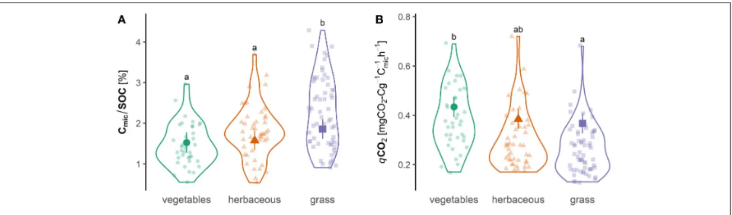
The Cmic/SOC ratio was lowest in vegetables and highest in
grass sites, while the qCO2 was lowest in grass and highest
in vegetable sites (Figure 4). The amount of “bare soil” was positively correlated with qCO2(r = 0.36, P < 0.001, Table S9)
and negatively with the Cmic/SOC ratio (r = −0.35, P < 0.001).
The structural soil quality indicator fromJohannes et al. (2017)
revealed that 85% of the gardens (Figure S2) had a SOC/clay ratio >1:13 and 4% were below the 1:10 threshold.
4. DISCUSSION
4.1. Soil Quality Assessment
Along with the ongoing discussion about the effect of urbanization on plant communities and soil properties (Groffman et al., 2017), we have found that garden habitats showed distinct MSQ. Thus, the way gardeners manage their habitats acts as an important driver of soil properties. In contrast to Edmondson et al. (2014), who found no differences in topsoil contents of SOC, TON, BD, and C/N ratio between soils of allotment, home and non-domestic green spaces, we found distinct differences in physical, chemical and biological MSQ (Table 3) between allotment and home gardens but most pronounced between the contrastingly managed habitat types. This conforms with the first hypothesis, that garden management practices have an effect on soil properties. Our second hypothesis that biological soil quality measures will be most affected by
T A B L E 3 | U n iv a ria te st a tis tic o f so il q u a lit y m e a su re s, u se d fo r th e so il q u a lit y a ss e ss m e n t a n d a d d iti o n a lv a lu e s o f te a b a g d e c o m p o si tio n a n d h e a vy m e ta ls . M e a n c v M e a n v e g e ta b le s M e a n h e rb a c e o u s M e a n g ra s s H e rb a c e o u s G ra s s H o me O v e rw a rmi n g E s ti ma te s e p E s ti ma te s e p E s ti ma te s e p E s ti ma te s e p P H Y S IC A L C la y [% ] 2 4 .0 ± 0 .5 2 3 2 4 .4 ± 0 .8 2 2 .9 ± 0 .8 2 4 .5 ± 0 .8 − 1 .0 9 ± 1 .0 3 0 .2 9 − 0 .0 3 ± 0 .9 3 0 .9 8 0 .2 1 ± 1 .1 5 0 .8 6 − 1 .1 4 ± 0 .5 6 0 .0 4 W a te r h o ld in g c a p a c ity (W H C ) [% ] 0 .8 2 ± 0 .0 1 1 6 0 .8 3 ± 0 .0 2 0 .8 1 ± 0 .0 2 0 .8 2 ± 0 .0 2 0 .0 2 ± 0 .0 2 0 .3 6 0 .0 2 ± 0 .0 2 0 .3 8 − 0 .0 4 ± 0 .0 3 0 .1 3 0 .0 2 ± 0 .0 1 0 .1 9 B u lk d e n si ty (B D ) [g c m − 3] 1 .0 7 ± 0 .0 1 1 5 1 .1 4 ± 0 .0 2 1 .1 1 ± 0 .0 3 1 .0 1 ± 0 .0 2 − 0 .0 5 ± 0 .0 3 0 .1 6 − 0 .1 4 ± 0 .0 3 < 0 .0 0 1 0 ± 0 .0 3 0 .9 7 − 0 .0 1 ± 0 .0 1 0 .7 3 M e a n p e n e tr a tio n re si st a n c e [M P a ] 1 .4 4 ± 0 .0 5 4 0 0 .9 8 ± 0 .0 7 1 .4 6 ± 0 .0 8 1 .7 ± 0 .0 7 0 .3 5 ± 0 .0 9 < 0 .0 0 1 0 .6 4 ± 0 .0 8 < 0 .0 0 1 0 .1 ± 0 .1 0 .3 2 0 .1 6 ± 0 .0 5 0 .0 1 S o il d e p th [c m ] 4 4 .0 ± 1 .6 4 3 5 0 .2 ± 2 .8 4 1 .1 ± 2 .6 4 2 .5 ± 2 .6 − 6 .1 6 ± 2 .8 2 0 .0 3 − 7 .6 8 ± 2 .4 9 0 .0 1 − 1 .9 6 ± 4 .1 1 0 .6 4 − 3 .8 3 ± 2 .0 0 0 .0 6 S ta b le a g g re g a te s (S A ) [% ] 8 3 .4 6 ± 0 .8 1 2 7 9 .2 4 ± 1 .6 8 2 .0 7 ± 1 .4 5 8 7 .0 0 ± 1 .1 2 .7 ± 1 .8 8 0 .1 6 7 .2 3 ± 1 .7 2 < 0 .0 0 1 3 .1 1 ± 1 .8 6 0 .1 0 0 .0 6 ± 0 .8 9 0 .9 5 C H E M IC A L p H 7 .2 6 ± 0 .0 2 3 7 .2 5 ± 0 .0 4 7 .3 2 ± 0 .0 3 7 .2 3 ± 0 .0 4 − 0 .0 2 ± 0 .0 4 0 .6 8 − 0 .0 7 ± 0 .0 4 0 .0 6 0 .1 5 ± 0 .0 5 0 .0 1 − 0 .0 2 ± 0 .0 3 0 .5 7 E le c tr ic a lc o n d u c tiv ity (E C ) [µ S c m − 1] 1 8 5 .4 ± 3 .3 2 2 1 7 7 .9 ± 7 .5 1 8 7 .3 ± 6 .3 1 8 8 .5 ± 4 .2 3 .9 ± 8 .1 9 0 .6 3 5 .6 9 ± 7 .4 8 0 .4 5 1 4 .6 8 ± 7 .9 8 0 .0 7 1 .6 7 ± 3 .8 2 0 .6 6 P [m g kg − 1] 1 8 0 .5 ± 9 .5 6 3 2 6 0 .6 ± 1 7 .8 1 7 2 .4 ± 1 6 .1 1 3 8 .6 ± 1 2 .3 − 6 7 .0 8 ± 2 0 .1 7 0 .0 1 − 1 0 9 .9 4 ± 1 8 .2 7 < 0 .0 0 1 − 5 9 .1 8 ± 2 1 .2 2 0 .0 1 1 5 .8 9 ± 1 0 .2 1 0 .1 2 K [m g kg − 1] 1 6 3 .5 ± 1 0 .4 7 6 2 2 2 .9 ± 2 2 .9 1 6 2 .2 ± 1 7 .1 1 2 9 .0 ± 1 4 .1 − 5 3 .7 6 ± 2 6 .4 2 0 .0 4 − 8 7 .5 3 ± 2 4 .5 5 < 0 .0 0 1 − 3 9 .3 6 ± 2 2 .4 9 0 .0 8 1 8 .5 5 ± 1 0 .6 3 0 .0 8 M g [m g kg − 1] 5 1 6 .0 ± 1 4 .6 3 4 5 6 5 .5 ± 3 3 .9 5 0 8 .8 ± 2 0 .0 4 9 1 .8 ± 2 2 .7 − 4 6 .4 8 ± 2 6 .1 6 0 .0 8 − 8 5 .1 8 ± 2 3 .1 5 < 0 .0 0 1 4 2 .9 7 ± 3 7 .5 7 0 .2 6 − 4 8 .3 8 ± 1 8 .3 1 0 .0 1 F e [m g kg − 1] 3 6 7 .2 ± 9 .1 3 0 3 9 5 .5 ± 2 1 .5 3 7 0 .4 ± 1 5 .3 3 4 7 .9 ± 1 2 .4 − 1 3 .1 7 ± 1 7 .1 3 0 .4 4 − 4 1 .6 ± 1 5 .2 6 0 .0 1 − 5 7 .5 ± 2 1 .8 9 0 .0 1 4 4 .7 2 ± 1 0 .6 3 < 0 .0 0 1 C u [m g kg − 1] 3 1 .9 ± 2 .3 8 7 3 5 .5 ± 4 .4 3 1 .7 ± 4 .1 2 9 .9 ± 3 .6 − 0 .0 9 ± 2 .3 5 0 .9 7 − 4 .4 3 ± 2 .0 3 0 .0 3 − 2 1 .1 1 ± 6 .3 8 0 .0 1 9 .8 8 ± 3 .1 4 0 .0 1 M n [m g kg − 1] 2 9 3 .7 ± 9 .2 3 8 2 9 1 .9 ± 2 0 .2 2 7 9 .6 ± 1 3 .3 3 0 5 .3 ± 1 4 .9 − 2 .9 6 ± 1 5 .7 9 0 .8 5 1 7 .6 4 ± 1 3 .9 3 0 .2 1 2 9 .2 6 ± 2 4 .0 1 0 .2 3 − 3 4 .1 ± 1 1 .7 2 0 .0 1 B [m g kg − 1] 1 .3 6 ± 0 .0 6 5 3 1 .8 8 ± 0 .1 1 1 .3 4 ± 0 .1 1 .0 6 ± 0 .0 7 − 0 .4 ± 0 .1 2 0 .0 1 − 0 .7 2 ± 0 .1 1 < 0 .0 0 1 − 0 .3 7 ± 0 .1 3 0 .0 1 0 .1 3 ± 0 .0 6 0 .0 5 B IO L O G IC A L B a sa lr e sp ira tio n [µ g C O2 − C g − 1h − 1] 0 .2 4 ± 0 .0 1 4 7 0 .2 7 ± 0 .0 2 0 .2 4 ± 0 .0 2 0 .2 2 ± 0 .0 1 − 0 .0 2 ± 0 .0 2 0 .4 4 − 0 .0 5 ± 0 .0 2 0 .0 2 − 0 .0 1 ± 0 .0 2 0 .5 2 0 .0 1 ± 0 .0 1 0 .2 2 Cm ic [m g kg − 1] 8 1 4 .5 7 ± 2 2 .2 3 3 7 1 3 .0 6 ± 4 1 .4 7 9 6 .2 8 ± 3 6 .9 8 8 8 .7 2 ± 3 4 .1 7 5 .1 1 ± 5 1 .7 6 0 .1 5 1 5 7 .1 3 ± 4 7 .0 7 0 .0 1 1 1 9 .2 5 ± 5 2 .3 2 0 .0 3 − 2 7 .9 5 ± 2 5 .1 0 .2 7 Nm ic [m g kg − 1] 1 4 2 .2 9 ± 4 .4 3 7 1 1 8 .6 6 ± 7 .3 1 4 0 .7 6 ± 7 .4 1 5 7 .5 3 ± 6 .9 1 9 .3 2 ± 1 0 .1 4 0 .0 6 3 5 .5 9 ± 9 .2 3 < 0 .0 0 1 2 3 .5 7 ± 1 0 .2 1 0 .0 2 − 3 .9 2 ± 4 .9 0 .4 3 Nm in [m g kg − 1] 1 .7 8 ± 0 .1 6 5 1 .7 0 ± 0 .1 1 .8 4 ± 0 .2 1 .7 8 ± 0 .2 0 .2 1 ± 0 .2 3 0 .3 6 0 .0 9 ± 0 .2 0 .6 7 − 0 .2 7 ± 0 .2 4 0 .2 8 0 .0 8 ± 0 .1 2 0 .5 1 A n e c ic S R [in d .m − 2] 1 .2 6 ± 0 .1 7 1 1 .3 5 ± 0 .2 1 .4 8 ± 0 .1 1 .0 5 ± 0 .1 0 .1 8 ± 0 .1 9 0 .3 3 − 0 .2 6 ± 0 .1 7 0 .1 4 − 0 .1 2 ± 0 .1 7 0 .4 7 − 0 .0 2 ± 0 .0 8 0 .7 7 A n e c ic M [g m − 2] 7 .9 3 ± 0 .5 8 0 7 .5 2 ± 0 .9 8 .7 8 ± 1 .2 7 .5 5 ± 0 .7 1 .5 2 ± 1 .3 8 0 .2 7 0 .1 ± 1 .2 7 0 .9 4 0 .4 9 ± 1 .2 6 0 .7 0 − 0 .4 8 ± 0 .6 0 .4 3 E n d o g e ic S R [in d .m − 2] 1 .7 3 ± 0 .1 7 3 2 .2 7 ± 0 .2 1 .5 9 ± 0 .1 1 .5 2 ± 0 .2 − 0 .5 3 ± 0 .2 6 0 .0 4 − 0 .7 5 ± 0 .2 4 0 .0 1 − 0 .1 1 ± 0 .2 5 0 .6 6 − 0 .1 3 ± 0 .1 2 0 .2 8 E n d o g e ic M [g m − 2] 3 .3 1 ± 0 .3 9 3 5 .1 5 ± 0 .7 2 .7 4 ± 0 .4 2 .6 5 ± 0 .3 − 2 .2 7 ± 0 .6 4 < 0 .0 0 1 − 2 .5 3 ± 0 .5 9 < 0 .0 0 1 − 0 .0 8 ± 0 .5 6 0 .8 8 − 0 .0 7 ± 0 .2 7 0 .8 0 E p ig e ic S R [in d .m − 2] 0 .6 2 ± 0 .1 9 2 0 .4 3 ± 0 .1 0 .8 3 ± 0 .1 0 .6 4 ± 0 .1 0 .0 0 1 ± 0 .0 0 1 1 .0 0 0 .0 0 1 ± 0 .0 0 1 1 .0 0 − 0 .3 3 ± 0 .3 1 .0 0 0 .0 6 ± 0 .1 8 1 .0 0 E p ig e ic M [g m − 2] 3 .4 3 ± 0 .4 1 3 0 1 .4 3 ± 0 .3 4 .2 6 ± 0 .6 4 .2 4 ± 0 .7 4 .2 8 ± 2 .2 7 0 .0 7 2 .6 6 ± 1 .7 8 0 .1 6 − 3 .2 6 ± 2 .2 7 0 .1 7 − 0 .0 8 ± 1 .0 0 0 .9 4 E a rt h w o rm S R [in d .m − 2] 3 .1 ± 0 .2 5 7 3 .7 ± 0 .3 3 .1 7 ± 0 .3 2 .6 8 ± 0 .2 − 0 .3 2 ± 0 .3 6 0 .3 8 − 0 .9 9 ± 0 .3 3 0 .0 1 − 0 .2 9 ± 0 .3 5 0 .4 1 − 0 .1 ± 0 .1 7 0 .5 5 E a rt h w o rm M [g m − 2] 1 2 5 .5 2 ± 7 .2 6 9 1 4 1 .0 5 ± 1 4 .8 1 2 8 .5 5 ± 1 5 .2 1 1 4 ± 8 .9 − 7 .9 ± 1 8 .8 3 0 .6 8 − 2 6 .8 4 ± 1 7 .3 4 0 .1 2 4 .0 8 ± 1 7 .0 9 0 .8 1 − 5 .9 3 ± 8 .1 3 0 .4 7 E a rt h w o rm a b u n d a n c e [in d .m − 2] 2 2 7 .3 5 ± 1 5 .5 8 2 3 3 6 .6 3 ± 4 0 .8 1 8 3 .5 7 ± 2 0 .8 1 9 4 .6 2 ± 1 8 .5 − 1 3 5 .7 9 ± 3 8 .7 2 < 0 .0 0 1 − 1 3 4 .4 5 ± 3 5 .9 1 < 0 .0 0 1 − 1 6 .2 2 ± 3 3 .5 1 0 .6 3 − 1 9 .2 9 ± 1 5 .8 6 0 .2 3 S O M S O C [% ] 4 .7 1 ± 0 .1 3 5 5 .1 8 ± 0 .3 4 .8 2 ± 0 .2 4 .3 6 ± 0 .2 − 0 .1 5 ± 0 .2 8 0 .5 9 − 0 .6 3 ± 0 .2 5 0 .0 1 − 0 .5 5 ± 0 .3 5 0 .1 2 0 .3 9 ± 0 .1 7 0 .0 2 T O N [% ] 0 .3 3 ± 0 .0 1 3 4 0 .3 6 ± 0 .0 2 0 .3 3 ± 0 .0 2 0 .3 2 ± 0 .0 1 − 0 .0 2 ± 0 .0 2 0 .2 9 − 0 .0 3 ± 0 .0 2 0 .1 0 − 0 .0 3 ± 0 .0 2 0 .2 3 0 .0 1 ± 0 .0 1 0 .5 7 P e a k A [A .U .c m − 1] 1 .2 3 ± 0 .0 3 3 2 1 .0 2 ± 0 .0 5 1 .2 5 ± 0 .0 6 1 .3 4 ± 0 .0 5 0 .2 5 ± 0 .0 8 0 .0 1 0 .3 5 ± 0 .0 7 < 0 .0 0 1 − 0 .1 3 ± 0 .0 7 0 .0 8 0 .0 6 ± 0 .0 4 0 .1 2 (C o n ti n u e d )
T A B L E 3 | C o n tin u e d M e a n c v M e a n v e g e ta b le s M e a n h e rb a c e o u s M e a n g ra s s H e rb a c e o u s G ra s s H o me O v e rw a rmi n g E s ti ma te s e p E s ti ma te s e p E s ti ma te s e p E s ti ma te s e p P e a k B [A .U .c m − 1] 0 .0 7 ± 0 .0 0 1 2 4 0 .0 6 ± 0 .0 0 1 0 .0 7 ± 0 .0 0 1 0 .0 7 ± 0 .0 0 1 0 .0 0 1 ± 0 .0 0 1 0 .2 4 0 .0 1 ± 0 .0 0 1 0 .0 3 0 .0 0 1 ± 0 .0 0 1 0 .7 3 0 .0 0 1 ± 0 .0 0 1 0 .2 5 P e a k C [A .U .c m − 1] 0 .3 3 ± 0 .0 1 2 4 0 .3 1 ± 0 .0 1 0 .3 4 ± 0 .0 1 0 .3 4 ± 0 .0 1 0 .0 2 ± 0 .0 2 0 .3 2 0 .0 2 ± 0 .0 1 0 .2 1 0 .0 2 ± 0 .0 2 0 .2 9 − 0 .0 1 ± 0 .0 1 0 .3 1 P e a k D [A .U .c m − 1] 0 .9 ± 0 .0 3 3 6 0 .9 1 ± 0 .0 5 0 .9 6 ± 0 .0 4 0 .8 6 ± 0 .0 5 0 .0 3 ± 0 .0 5 0 .5 2 − 0 .0 4 ± 0 .0 5 0 .3 6 − 0 .0 2 ± 0 .0 7 0 .8 1 0 .0 5 ± 0 .0 3 0 .1 5 S O IL Q U A L IT Y IN D IC E S Cm ic /S O C [% ] 1 .9 ± 0 .0 7 4 2 1 .4 7 ± 0 .0 9 1 .7 8 ± 0 .1 2 .2 4 ± 0 .1 1 0 .2 5 ± 0 .1 3 0 .0 6 0 .6 8 ± 0 .1 2 < 0 .0 0 1 0 .4 6 ± 0 .1 5 0 .0 1 − 0 .1 9 ± 0 .0 7 0 .0 1 q C O2 [µ g C O2 − C g − 1h − 1C − 1 m ic h − 1] 0 .3 1 ± 0 .0 1 4 0 0 .3 8 ± 0 .0 2 0 .3 ± 0 .0 2 0 .2 7 ± 0 .0 1 − 0 .0 6 ± 0 .0 2 0 .0 1 − 0 .1 ± 0 .0 2 < 0 .0 0 1 − 0 .0 6 ± 0 .0 2 0 .0 1 0 .0 2 ± 0 .0 1 0 .0 4 S O C /c la y 0 .2 1 ± 0 .0 1 4 5 0 .2 3 ± 0 .0 2 0 .2 2 ± 0 .0 1 0 .1 9 ± 0 .0 1 0 ± 0 .0 2 0 .9 1 − 0 .0 3 ± 0 .0 2 0 .0 5 − 0 .0 2 ± 0 .0 2 0 .2 3 0 .0 3 ± 0 .0 1 0 .0 1 T B I G re e n te a d e c o m p o si tio n [% ] 5 9 .0 ± 3 .7 7 5 7 .7 ± 7 .1 5 8 .5 ± 5 .8 6 0 .1 ± 5 .8 0 .0 1 ± 0 .0 1 0 .6 1 0 .0 2 ± 0 .0 1 0 .0 1 − 0 .0 1 ± 0 .0 1 0 .4 4 0 .0 1 ± 0 .0 0 1 0 .0 2 R o o ib o s te a d e c o m p o si tio n [% ] 2 9 .6 ± 2 .8 1 1 2 9 .4 ± 4 .9 2 9 .8 ± 5 .4 2 9 .5 ± 4 .2 0 .0 0 1 ± 0 .0 1 0 .9 9 0 .0 0 1 ± 0 .0 1 0 .7 8 0 .0 1 ± 0 .0 1 0 .3 6 0 .0 0 1 ± 0 .0 0 1 0 .4 4 H E A V Y M E T A L S S b [m g kg − 1] 1 .9 1 ± 0 .4 2 3 1 2 .4 7 ± 0 .9 1 .6 2 ± 0 .3 1 .7 9 ± 0 .6 − 1 .3 5 ± 0 .8 8 0 .1 3 − 0 .7 4 ± 0 .8 0 .3 5 0 .8 7 ± 0 .9 2 0 .3 5 − 0 .1 4 ± 0 .4 4 0 .7 5 A s [m g kg − 1] 9 .4 1 ± 0 .3 3 7 8 .8 5 ± 0 .7 9 .5 5 ± 0 .5 9 .6 3 ± 0 .4 0 .0 1 ± 0 .4 3 0 .9 9 0 .5 1 ± 0 .3 8 0 .1 8 0 .8 9 ± 0 .8 1 0 .2 7 − 0 .3 9 ± 0 .4 0 .3 3 C o [m g kg − 1] 3 1 .6 0 ± 0 .4 1 5 3 1 .3 1 ± 0 .8 3 2 .6 2 ± 0 .7 3 1 .0 2 ± 0 .6 0 .6 4 ± 0 .9 4 0 .5 0 − 0 .7 2 ± 0 .8 6 0 .4 0 2 .3 8 ± 0 .9 4 0 .0 1 − 1 .1 ± 0 .4 5 0 .0 2 C u [m g kg − 1] 7 7 .3 0 ± 4 .9 7 7 8 5 ± 9 .0 7 7 .4 4 ± 9 .0 7 2 .6 ± 7 .8 − 9 .3 2 ± 5 .7 9 0 .1 1 − 1 2 .5 9 ± 5 .0 2 0 .0 1 − 4 .7 7 ± 1 4 .2 8 0 .7 4 8 .0 6 ± 7 .0 2 0 .2 5 P b [m g kg − 1] 1 7 9 .1 4 ± 1 5 .0 1 0 1 1 9 5 .4 7 ± 2 7 .5 1 7 1 .5 4 ± 2 4 .0 1 7 5 .0 2 ± 2 5 .7 − 1 5 .0 6 ± 2 8 .5 3 0 .6 0 − 1 0 .5 1 ± 2 5 .2 7 0 .6 8 − 1 5 .5 2 ± 4 0 .1 6 0 .7 0 8 .2 2 ± 1 9 .5 6 0 .6 8 V [m g kg − 1] 7 9 .4 0 ± 1 .3 1 9 7 5 .7 3 ± 2 .2 8 1 .7 2 ± 2 .3 7 9 .8 8 ± 2 .0 2 .9 7 ± 2 .4 0 .2 2 3 .4 5 ± 2 .1 3 0 .1 1 7 .0 8 ± 3 .2 2 0 .0 3 − 4 .4 1 ± 1 .5 7 0 .0 1 Es ti m a te s a n d p -v a lu e s a re re po rte d fr o m lin e a r m ix e d e ff e c t m ode ls w ith ov e rw a rm in g, ga rde n h a bi ta t, a n d ga rde n ty pe a s fix e d e ff e c ts a n d ga rde n ide n ti ty a s ra n dom e ff e c t. B ol d va ri a bl e s in di c a te p < 0.05. M, e a rth w or m bi om a s s ; S R , e a rth w o rm s pe c ie s ri c h n e s s ; c v, c o e ffi c ie n t o f va ri a ti on .
FIGURE 4 | Violin plots showing probability density of the raw data of (A) Microbial quotient Cmic/SOC and (B) the metabolic quotient qCO2. Colors correspond to the different garden habitat types with the following observation numbers: Annual vegetables (N = 37), perennial herbaceous (N = 46), and perennial grass (N = 62). Bold points are mean values of the simulated Bayesian inference posterior distribution taking into account the random effect of garden identity with the 95% credible intervals as lines. Letters are least square means from linear mixed effect models (cf. Table S11) with a significance level alpha = 0.05.
garden management practices could not be confirmed, since other measures, such as physiochemical soil properties were equally important in the NMDS ordination. This underpins the importance of assessing soil quality with a comprehensive set of inherent and dynamic soil quality measurements. Overall, our results support the importance of anthropogenic management in urban ecology theory (Alberti, 1999), but we found little evidence for a convergence of soil properties with urbanization contrary to the urban convergence hypothesis of McKinney (2006). Whereas,Pouyat et al. (2015)found that topsoil contents of SOC and TON converged, but others such as K and P rather diverged in five metropolitan areas. In contrast to this study we found higher SOC with increasing urbanization density. This may be explained by less intensive managed urban gardens such as more grass sites in the inner parts of Zurich. Our results support the findings ofGreinert (2015), that variation in soil properties increases with anthropogenic management and land-use types. The urban convergence theory does not take ecosystem services into account, therefore further research is needed to close this gap. Similar to the findings ofPouyat and Carreiro (2003), who showed increased litter decomposition rates in urban than in rural forests, we found a positive correlation of decomposition and urbanization density. This might be due to the enhanced microbial decomposer activity caused by the UHI effect (Craine et al., 2010).
It has been proven that ecological gardening practices such as the application of organic inputs (Cogger, 2005; Sax et al., 2017) or less soil disturbance in gardens (Grewal et al., 2011) contribute to the above-ground biodiversity (e.g., Fuller et al., 2007; Sperling and Lortie, 2010). Further consequences on the nutrient cycle or soil quality are still poorly explored. We could show that sites with frequent compost application had higher P contents, endogeic earthworm species richness and biomass as well as lower penetration resistance. Other studies showed that organic matter inputs such as compost or mulch improved physical soil properties (Beniston and Lal, 2012). We support the fact that compost is a valuable regenerative soil management practice, but its quality must be tested, as urban
organic waste may contain soil contaminants (Alvarenga et al., 2015).
In general, our results confirm the findings of Edmondson et al. (2014)that soil quality can be better in urban gardens than in agricultural soils. For example, topsoil content of Cmic, was
on average 57% higher (cf. Table 4) than the reference values for Swiss croplands (Oberholzer et al., 1999), but was still 2.5 times lower than extensive grassland values (Oberholzer and Scheid, 2007). Similarly, Nmic content was found to be 82% higher
than Swiss croplands (Oberholzer et al., 1999) but four times lower than extensive grassland values (Oberholzer and Scheid, 2007). The mean density of 225 earthworms per m2was higher compared to conventionally tilled Swiss agricultural soils (Kuntz et al., 2013) but at the same level as urban soils in Neuchâtel (CH) found byAmossé et al. (2016). The mean biomass of earthworms was lower by a factor of 2.4 compared to the reference value for Swiss grasslands (Stähli et al., 1997). This is probably because agricultural fields are dominated by anecic earthworm species, known to have a high body weight and abundance (Bouché, 1977). Bulk density was 13% lower and stable soil aggregates were 51% higher in comparison with agricultural soils (Mäder et al., 2002) and nutrient contents such as P or K have been enriched by a factor of 8.4 and 1.7, respectively.
4.2. Effect of Soil Disturbance on Urban
Garden Soils
Overall, we found that intensive soil management such as the use of pesticides and fertilizers were associated with higher values of respiration rates and labile compounds of SOM (Figure 3). We hypothesized that more intense soil management results in a lower Cmic/SOC ratio and a higher qCO2. We
observed lower Cmic/SOC and higher qCO2 values (Figure 4)
in vegetables than in the less frequently disturbed grass sites, which is comparable with the findings ofAnderson (2003)who reported higher Cmic/SOC and lower qCO2values for soils under
crop rotation. However, these two indices cannot discriminate between disturbed or stressed (e.g., nutrient poor) ecosystems but are still valuable bio-indicators of soil quality (Wardle and
TABLE 4 | Comparison of selected physical, chemical, and biological properties of urban soils compared to other urban studies or reference values from Swiss agricultural topsoils.
This study Other studies References
PHYSICAL PROPERTIES
Stable aggregates [%] Vegetables 77.3 ± 1.8 55 Conventional agricultural fields, CHE Mäder et al., 2002
Herbaceous 82.7 ± 1.4
Grass 87 ± 1.1
Mean 83 ± 0.8
Bulk density [g cm−3] Vegetables 1.15 ± 0.02 1.09 Urban garden soils, Bottrop, GER Burghardt and Schneider, 2016 Herbaceous 1.10 ± 0.03 1.23 Conventional agricultural fields, CHE Mäder et al., 2002
Grass 1.01 ± 0.02
Mean 1.07 ± 0.01
CHEMICAL PROPERTIES
Phosphorus [mg kg−1] Vegetables 247.5 ± 16.6 21.4 Conventional agricultural fields, CHE Mäder et al., 2002
Herbaceous 176.0 ± 16.6 90 ± 15 Urban cites including gardens of Baltimore, USA Pouyat et al., 2007
Grass 138.7 ± 12.4
Mean 179.2 ± 9.3
Kalium [mg kg−1] Vegetables 212.2 ± 22.1 97.5 Conventional agricultural fields, CHE Mäder et al., 2002 Herbaceous 166.6 ± 17.5 106 ± 5.2 Urban cites including gardens of Baltimore, USA Pouyat et al., 2007
Grass 129.16 ± 14.1
Mean 162.8 ± 10.3
Lead [mg kg−1] Vegetables 181.3 ± 26.8 36 European agricultural soils GEMAS, EU Reimann et al., 2012
Herbaceous 175.7 ± 24.9 74.6 Vegetable garden soils three french cities, FRA Joimel et al., 2016
Grass 175.0 ± 25.7 202 Urban parks Palermo, ITA Salvagio Manta et al., 2002
Mean 176.9 ± 15.1 231 ± 53 Urban cites including gardens of Baltimore, USA Pouyat et al., 2007
266 Garden soils of 50 UK cities, GBR Alloway, 2004
291 Urban garden soils, Bottrop, GER Burghardt and Schneider, 2016
BIOLOGICAL PROPERTIES
Cmic[mg kg−1] Vegetables 699.1 ± 39.9 321 Urban park soils of Aberdeen, GBR Yuangen et al., 2006 Herbaceous 808.6 ± 37.5 518 Reference values Swiss cropland, CHE Oberholzer et al., 1999
Grass 888.7 ± 34.1 2077 Reference values Swiss grassland extensive, CHE Oberholzer and Scheid, 2007
Mean 813.2 ± 22.4
Nmic[mg kg−1] Vegetables 116.3 ± 7.0 78 Reference values Swiss cropland, CHE Oberholzer et al., 1999 Herbaceous 142.9 ± 7.5 573 Reference values Swiss grassland extensive, CHE Oberholzer and Scheid, 2007
Grass 157.5 ± 6.8
Mean 142.0 ± 42
SOC [%] Vegetables 5.0 ± 0.3 2.6 Vegetable garden soils three french cities, FRA
Herbaceous 4.9 ± 0.2 2.9 Urban park soils of Aberdeen, GBR Yuangen et al., 2006
Grass 4.3 ± 0.2 5.2 Urban soils of Neuchâtel, CHE Amossé et al., 2016
Mean 4.7 ± 0.1 5.2 Allotment gardens (vegetable beds) GER Burghardt and Schneider, 2016
5.8 Allotment gardens (lawn), GER Burghardt and Schneider, 2016
Earthworm density [ind. m−2] Vegetables 321 ± 40 25 Urban-rural oak forest stands New York City, USA Steinberg et al., 1997
Herbaceous 183 ± 22 54 Conventional agricultural fields, CHE Kuntz et al., 2013
Grass 195 ± 18 93 Floodplains, Thur river, CHE Fournier et al., 2012
Mean 225 ± 18 220 Urban soils of Neuchâtel, CHE Amossé et al., 2016
Earthworm biomass [g m−2] Vegetables 133.3 ± 14.9 301 Reference values Swiss grassland sites, CHE Stähli et al., 1997
Herbaceous 127.6 ± 15.9
Grass 114.0 ± 8.9
Mean 123.3 ± 7.3
Total earthworm species Vegetables 13 13 Urban parks Basel, CHE Glasstetter and Nagel, 2001
Herbaceous 15 18 Urban cites including gardens of Baltimore, USA Pouyat et al., 2010
Grass 15 19 Urban sites Brussels, BEL Pižl and Josens, 1995
Total 18
Ghani, 2018). Inspired by Johannes et al. (2017) we found increased SOC/clay ratios compared to agriculture sites, but this relationship must be further investigated for other non-arable soils.
4.3. Heavy Metal Assessment
Soil contamination is a potential health risk for gardeners who consume their own vegetables and especially for children who play on the ground and ingest contaminated soil directly (Kim et al., 2014). Soil contamination varies widely and depends on emission sources such as industry (Salvagio Manta et al., 2002) and traffic (Filippelli and Laidlaw, 2010; Beniston and Lal, 2012) but also on geogenic factors. Pb contamination in urban soils is mainly due to historical use of leaded paint, vehicle (Chaney and Ryan, 1994) and industrial emissions (Beniston and Lal, 2012). Although the use of Pb is strongly restricted today, it still represents a serious risk for human health due to its high persistence in soils (Filippelli and Laidlaw, 2010). Total Pb concentrations in urban gardens worldwide vary widely (e.g., from 60 to > 2,500 mg kg−1; Cheng et al., 2011; Attanayake et al., 2014), this is also confirmed in this study, whereby the concentrations ranged between 18.5 and 1,076 mg kg−1. Nonetheless, the mean value of Pb was relatively low compared to other cities (Table 4). A potential public health risk exists in soils with >1,000 mg kg−1 Pb (Whitzling et al., 2010), which
makes them unsuitable for urban gardening (Beniston and Lal, 2012). This is also the upper guideline limit for Pb in Swiss soils (Swiss Federal Council, 1998), which was exceeded only once in this study. The threshold requiring a further inspection of the soils (300 mg Pb kg−1) was exceeded in 16% of all garden
sites (18 allotments and 10 home gardens), thus requiring further examination. It has to be mentioned, that the XRF device rather overestimates heavy metal concentrations by 10–20% compared to the standard method with aqua regia digestion (Christl et al., 2004).
We assumed that heavy metals had a negative impact on decomposition and functional groups of earthworms, but no correlation was found. A possible explanation is that the positive influence of garden management particularly the high SOM content, may have masked potentially toxic effects (Fliessbach et al., 1994). Besides that, we found positive correlations of Cu, Pb, and Sb with the “slope” as well as the broad scale spatial variable “MEM2” (Figure S9). The latter can be interpreted as an increased exposure to industrial facilities in the North Eastern parts of Zurich. A certain bias of our results may derive from the fact, that the survey questions represent only the current but not the past management practices. While we have focused on heavy metals, there are other contaminations common to urban areas, such as polycyclic aromatic hydrocarbons and polychlorinated biphenyls (Vane et al., 2014), which can have negative impact on urban food production and therefore should be addressed in future studies.
4.4. Gardening Effects on Functional
Groups of Earthworms and Decomposition
It has been shown that the loss of soil biota has a negative impact on soil functions and thus also on the health of ecosystems in natural soils (Handa et al., 2014). We found that garden
management not only influences soil quality, but also functional groups of earthworms. Surprisingly, we found the highest diversity and biomass of earthworms in vegetable sites that are more frequently disturbed than grass sites. Although intensive agricultural soil management practices adversely affect total earthworm species numbers (Smith et al., 2008), the impacts may also depend on ecological groups of earthworms. For example, the number of endogeic species can also increase with tillage due to increased food supply, while the abundance of deep burrowing anecic species decreases (Chan, 2000). This could also explain the positive correlation between “bare soil” and endogeic biomass. Interestingly, “compost” was also positively related to endogeic earthworms, highlighting the importance of providing food to earthworms. In contrast to the study carried out in urban forests of New York (Steinberg et al., 1997), we found no correlation between earthworm abundance and urban density. Moreover, we found higher decomposition rates in grass than in vegetables sites (Table 3, Table S11), unlikeGrewal et al. (2011) who reported no differences in the decomposition rates between vacant lots, mainly consisting of grass sites and urban gardens, dominated by vegetables and fruits. With the modification of the TBI protocol given byKeuskamp et al. (2013), we tried to minimize bias in mass loss due to small soil particles which could enter the mesh size of the tea bags. However, this did not prevent from possible ingrowth of fungal hyphae, representing a deficiency of the TBI method. Beyond that,Pelosi et al. (2016)observed that functional but not structural diversity decreases with soil tillage intensity. Therefore, future research on the effects of soil management on soil fauna should not only focus on structural but also on functional diversity.
4.5. Conclusion
Soil is essential for the functioning of urban ecosystems (Levin et al., 2017). Although urban garden soils are an important part of urban green spaces, they are still poorly investigated. The multivariate approach has allowed for an integrated and comprehensive evaluation of the impact of garden management on soil quality. Garden management was identified as the main driver of the differentiation of gardens according to soil quality. Our results show the fragmentation of soil quality within a garden and the city, which was mainly dependent on the habitat (annual vegetables, herbaceous, and perennial grass). Other gardening practices, such as mulching or the use of compost, improve soil quality, whereas soil disturbance such as frequent digging and compaction may change soil biological activity. The eco-physiological indicators of soil quality qCO2
and Cmic/SOC were useful in identifying soil disturbance and
the intensity of soil use, indicating diverging biogenic soil quality properties in contrastingly managed urban garden soils. Moreover, we found that the gardening practices lead to an increased SOC/clay ratio indicating a higher structural soil quality and that biological measures of soil quality such as Cmicor
earthworm densities and species richness are strongly increased compared to agricultural soils. The multivariate approach by combining management, garden as well as city characteristics with soil quality measurements, allowed for disentangling the gardener’s impact on urban soils. This may also be applied to other research questions focussing on soil quality in urban as well
as in rural areas. In summary, this study contributes to a better understanding of the role of garden soils in urban ecosystems and provides inputs for a sustainable management practice of garden soils.
DATA AVAILABILITY STATEMENT
All data generated for this study is part of the interdisciplinary research project BetterGardens. Data supporting the conclusions of this manuscript will be made available by the authors, upon request to any qualified researcher.
AUTHOR CONTRIBUTIONS
AF, MM, R-CL, PM DF, and ST: conceived and designed the research; DF, AZ, and ST: performed the field work; ST: performed the lab work and analyzed the data. All authors contributed to the writing of the manuscript.
FUNDING
We gratefully acknowledge the financial support for this interdisciplinary project BetterGardens provided by the Swiss
National Science Foundation in frame of the Sinergia programm (CRSII1_154416).
ACKNOWLEDGMENTS
We thank the project coordinator Dr. Robert Home and the whole BetterGardens team. We are grateful to Prof. Rainer Schulin (XRF analysis), Dr. Frank Rasche and Dr. Scott Demian (DRIFTS analysis), Dr. Lukas Pfiffner (earthworm identification) as well as to Dr. Daniel Haefelfinger, Adolphe Munyangabe, Anton Kuhn, Lena Fischer, Stefan Grubelnig, Reto Henzmann, Bernhard Stehle, Rebekka Tresch, Roger Köchlin and Björn Studer for their extraordinary support in the field and lab work. We acknowledge in particular the willingness and interest of the 85 participating gardeners of this study, who provided access and let us dig and sample soils in their gardens.
SUPPLEMENTARY MATERIAL
The Supplementary Material for this article can be found online at: https://www.frontiersin.org/articles/10.3389/fenvs. 2018.00025/full#supplementary-material
REFERENCES
Agroscope (2012). Referenzmethoden der Forschungsanstalten Agroscope: Band 1, Bodenuntersuchungen zur Düngeberatung. Zurich: Forschungsanstalt Agroscope Reckenholz-Tänikon (ART) and Changins-Wädenswil (ACW). Alberti, M. (1999). Modeling the urban ecosystem: a conceptual framework.
Environ. Plann. B 26, 605–630.
Alloway, B. J. (2004). Contamination of domestic gardens and allotments. Land Contam. Reclam. 12, 179–187. doi: 10.2462/09670513.658
Alvarenga, P., Mourinha, C., Farto, M., Santos, T., Palma, P., Sengo, J., et al. (2015). Sewage sludge, compost and other representative organic wastes as agricultural soil amendments: benefits versus limiting factors. Waste Manag. 40, 44–52. doi: 10.1016/j.wasman.2015.01.027
Amossé, J., Dózsa-Farkas, K., Boros, G., Rochat, G., Sandoz, G., Fournier, B., et al. (2016). Patterns of earthworm, enchytraeid and nematode diversity and community structure in urban soils of different ages. Eur. J. Soil Biol. 73, 46–58. doi: 10.1016/j.ejsobi.2016.01.004
Anderson, T. H. (2003). Microbial eco-physiological indicators to asses soil quality. Agric. Ecosyst. Environ. 98, 285–293. doi: 10.1016/S0167-8809(03)00088-4 Anderson, T.-H., and Domsch, K. (1989). Ratios of microbial biomass carbon to
total organic carbon in arable soils. Soil Biol. Biochem. 21, 471–479.
Attanayake, C. P., Hettiarachchi, G. M., Harms, A., Presley, D., Martin, S., and Pierzynski, G. M. (2014). Field evaluations on soil plant transfer of lead from an Urban garden soil. J. Environ. Qual. 43, 475–487. doi: 10.2134/jeq2013.07.0273 Baes, A. U., and Bloom, P. R. (1989). Diffuse reflectance and transmission Fourier transform infrared (DRIFT) spectroscopy of humic and fulvic acids. Soil Sci. Soc. Am. J. 53, 695–700.
Bartlett, M. D., Briones, M. J. I., Neilson, R., Schmidt, O., Spurgeon, D., and Creamer, R. E. (2010). A critical review of current methods in earthworm ecology: from individuals to populations. Eur. J. Soil Biol. 46, 67–73. doi: 10.1016/j.ejsobi.2009.11.006
Beniston, J., and Lal, R. (2012). “Improving soil quality for Urban agriculture in the North Central U.S.,” in Carbon Sequestration in Urban Ecosystems, eds R. Lal, and B. Augustin (Dordrecht: Springer), 279–313.
Beniston, J. W., Lal, R., and Mercer, K. L. (2016). Assessing and managing soil quality for Urban agriculture in a degraded vacant lot soil. Land Degrad. Dev. 27, 996–1006. doi: 10.1002/ldr.2342
Blakemore, R. (2008). An Updated List of Valid, Invalid and Synonym Names of Criodrioidea (Criodrilidae) and Lumbricoidea (Annelida: Oligochaeta: Spar-ganophilidae, Ailoscolecidae, Hormogastridae, Lumbricidae, and Luto- drilidae). Ph.D. thesis, Yokohama National University.
Bolund, P., and Hunhammar, S. (1999). Ecosystem services in urban areas. Ecol. Econ. 29, 293–301.
Borcard, D., Gillet, F., and Legendre, P. (2011). Numerical Ecology with R. New York, NY: Springer.
Bouché, M. (1977). Lombriciens de France. Ecologie et systématique. Paris: Annales de edition; INRA Editions.
Bowler, D. E., Buyung-Ali, L., Knight, T. M., and Pullin, A. S. (2010). Urban greening to cool towns and cities: a systematic review of the empirical evidence. Landsc. Urban Plann. 97, 147–155. doi: 10.1016/j.landurbplan.2010.05.006 Braaker, S., Ghazoul, J., Obrist, M. K., and Moretti, M. (2014). Habitat connectivity
shapes urban arthropod communities: the key role of green roofs. Ecology 95, 1010–1021. doi: 10.1890/13-0705.1
Bradley, R., Milne, R., Bell, J., Lilly, A., Jordan, C., and Higgins, A. (2005). A soil carbon and land use database for the United Kingdom. Soil Use Manage. 21, 363–369. doi: 10.1079/SUM2005351
Bünemann, E. K., Bongiorno, G., Bai, Z., Creamer, R. E., De Deyn, G., de Goede, R., et al. (2018). Soil quality - a critical review. Soil Biol. Biochem. 120, 105–125. doi: 10.1016/j.soilbio.2018.01.030
Burghardt, W., and Schneider, T. (2016). Bulk density and content, density and stock of carbon, nitrogen and heavy metals in vegetable patches and lawns of allotments gardens in the northwestern Ruhr area, Germany. J. Soils Sediments 18, 407–417. doi: 10.1007/s11368-016-1553-8
Chan, K. Y. (2000). An overview of some tillage impacts on earthworm population abundance and diversity - Implications for functioning in soils. Soil Tillage Res. 57, 179–191. doi: 10.1016/S0167-1987(00)00173-2
Chaney, R. L., and Ryan, J. A. (1994). Risk Based Standards for Arsenic, Lead and Cadmium in Urban Soils. Frankfurt: Dechema.
Cheng, Z., Lee, L., Dayan, S., Grinshtein, M., and Shaw, R. (2011). Speciation of heavy metals in garden soils: evidences from selective and sequential chemical leaching. J. Soils Sediments 11, 628–638. doi: 10.1007/s11368-011-0351-6 Christl, I., Gulz, P. A., Kretzschmar, R., and Schulin, H. R. (2004). Umgang mit
Bodenbelastungen in Familiengärten der Stadt Zürich. Technical report, ETH Zürich.