Spatial and temporal CO2 exchanges measured by Eddy Covariance over a temperate intertidal flat and their relationships to net ecosystem production

Biogeosciences, 9, 249–268, 2012 www.biogeosciences.net/9/249/2012/ doi:10.5194/bg-9-249-2012

© Author(s) 2012. CC Attribution 3.0 License.

Biogeosciences

Spatial and temporal CO

₂

exchanges measured by Eddy Covariance

over a temperate intertidal flat and their relationships to net

ecosystem production

P. Polsenaere1,*, E. Lamaud2, V. Lafon1, J.-M. Bonnefond2, P. Bretel1, B. Delille1,3, J. Deborde1,4, D. Loustau2, and G. Abril1,5

1_{Laboratoire Environnements et Pal´eoenvironnements OC´eanique (EPOC), Universit´e Bordeaux 1, CNRS-UMR5805,} Avenue des Facult´es, 33405 Talence Cedex, France

2_{Laboratoire Ecologie fonctionnelle et PHYSique de l’Environnement (EPHYSE), INRA, Centre de Bordeaux-Aquitaine, 71} Avenue Edouard Bourlaux, 33883 Villenave d’Ornon Cedex, France

3<sub>Unit´e Oc´eanographie Chimique, D´epartement d’Astrophysique, G´eophysique et Oc´eanographie, Universit´e de Li`ege, All´ee</sub> du 6 Aoˆut, 17-Bˆat. B5 4000 Li`ege, Belgium

4_{Institut de Recherche pour le D´eveloppement (IRD), 101 Promenade Roger Laroque-Anse Vata BPA5 98848 Noum´ea,} Nouvelle-Cal´edonie, France

5_{Institut de Recherche pour le D´eveloppement (IRD), Laboratorio de Potamologia Amazˆonica, LAPA, Universidade Federal} do Amazˆonas, Manaus, Brazil

*_{present address: Royal Netherlands Institute for Sea Research (NIOZ), Ecosystem Studies Department, Korringaweg 7, 4401} NT Yerseke, The Netherlands

Correspondence to: P. Polsenaere (p.polsenaere@nioo.knaw.nl, p.polsenaere@epoc.u-bordeaux1.fr)

Received: 23 May 2011 – Published in Biogeosciences Discuss.: 6 June 2011

Revised: 4 December 2011 – Accepted: 26 December 2011 – Published: 12 January 2012

Abstract. Measurements of carbon dioxide fluxes were

per-formed over a temperate intertidal mudflat in southwestern France using the micrometeorological Eddy Covariance (EC) technique. EC measurements were carried out in two con-trasting sites of the Arcachon flat during four periods and in three different seasons (autumn 2007, summer 2008, au-tumn 2008 and spring 2009). In addition, satellite images of the tidal flat at low tide were used to link the net ecosystem CO2exchange (NEE) with the occupation of the mudflat by primary producers, particularly by Zostera noltii meadows. CO2 fluxes during the four deployments showed important spatial and temporal variations, with the flat rapidly shift-ing from sink to source with the tide. Absolute CO2fluxes showed generally small negative (influx) and positive (efflux) values, with larger values up to −13 µmol m−2s−1 for in-fluxes and 19 µmol m−2s−1for effluxes. Low tide during the day was mostly associated with a net uptake of atmospheric CO2. In contrast, during immersion and during low tide at night, CO2fluxes where positive, negative or close to zero, depending on the season and the site. During the autumn of 2007, at the innermost station with a patchy Zostera noltii

bed (cover of 22 ± 14 % in the wind direction of measure-ments), CO2influx was −1.7 ± 1.7 µmol m−2s−1at low tide during the day, and the efflux was 2.7 ± 3.7 µmol m−2s−1 at low tide during the night. A gross primary production (GPP) of 4.4 ± 4.1 µmol m−2_s−1_{during emersion could be} attributed to microphytobenthic communities. During the summer and autumn of 2008, at the central station with a dense eelgrass bed (92 ± 10 %), CO2uptakes at low tide dur-ing the day were −1.5 ± 1.2 and −0.9 ± 1.7 µmol m−2s−1, respectively. Night time effluxes of CO2 were 1.0 ± 0.9 and 0.2 ± 1.1 µmol m−2s−1in summer and autumn, respec-tively, resulting in a GPP during emersion of 2.5 ± 1.5 and 1.1 ± 2.0 µmol m−2s−1, respectively, attributed primar-ily to the seagrass community. At the same station in April 2009, before Zostera noltii started to grow, the CO2 uptake at low tide during the day was the highest (-2.7 ± 2.0 µmol m−2s−1). Influxes of CO2 were also ob-served during immersion at the central station in spring and early autumn and were apparently related to phytoplank-ton blooms occurring at the mouth of the flat, followed by the advection of CO2-depleted water with the flooding tide.

250 P. Polsenaere et al.: Spatial and temporal CO2exchanges measured by Eddy Covariance

Although winter data as well as water carbon measurements would be necessary to determine a precise CO2budget for the flat, our results suggest that tidal flat ecosystems are a modest contributor to the CO2budget of the coastal ocean.

1 Introduction

The coastal zone is defined as the ocean area on the conti-nental shelf with a depth of less than 200 m, including all estuarine areas to the upstream limit of tidal influence. The coastal zone receives considerable amounts of nutrients and organic matter from the land, exchanges matter and energy with the open ocean (Borges, 2005) and thus constitutes one of the most biogeochemically active areas of the bio-sphere (Gattuso et al., 1998; Borges et al., 2005). In the coastal ocean, shallow depth favours light penetration in a large part of the water column and allows for a strong cou-pling between pelagic and benthic processes. These charac-teristics make the coastal zone very active in terms of CO2 exchange with atmosphere, benthic and pelagic primary pro-duction and respiration (Gazeau et al., 2004; Borges et al., 2006). The coastal zone covers approximately 7 % of the surface of the global ocean; despite its relatively modest sur-face area, this zone accounts for 14–30 % of all oceanic pri-mary production, 80 % of organic matter burial and 90 % of sedimentary mineralisation (Mantoura et al., 1991; Pernetta and Milliman, 1995). In addition, continental shelves act as a net sink of CO2of −0.21 ± 0.36 PgC yr−1– i.e. 15 % of the open ocean sink – whereas near-shore estuarine environ-ments emit to the atmosphere +0.27 ± 0.23 PgC yr−1 (Laru-elle et al., 2010). This active but heterogeneous region of the ocean has recently begun to be taken into account in global carbon budgeting efforts (Frankignoulle et al., 1998; Borges, 2005).

The ability of an ecosystem to consume CO2 and pro-duce organic matter is governed to a large extent by its net ecosystem production (NEP), defined either as the rate of net organic carbon burial and export or as the difference be-tween ecosystem-level gross primary production (GPP) and community respiration (CR) (Smith and Hollibaugh, 1993; Gattuso et al., 1998). GPP represents the C fixation by au-totrophic organisms, and CR represents the respiration of all organisms, both autotrophic and heterotrophic. Both GPP and CR are summed per unit ground or water area over time (Chapin et al., 2006). Autotrophic ecosystems have GPP greater than their CR and are net producers of organic C that can be accumulated in the system or exported outside of the system. Heterotrophic ecosystems have GPP lower than their CR and are net consumers of organic C supplied by an external source (Odum, 1956). GPP and CR are pro-cesses that also consume and release, on a short timescale, inorganic C in an ecosystem. In a terrestrial system, GPP directly consumes atmospheric CO2, and CR releases CO2

directly to the atmosphere. Thus, the net ecosystem ex-change (NEE), defined as the net vertical CO2exchange be-tween the ecosystem and the atmosphere, is generally ap-proximated by NEP in many terrestrial ecosystems over short timescales (Baldocchi, 2003). In contrast, in aquatic sys-tems, GPP consumes dissolved inorganic carbon and reduces the concentration of CO2 in the water. This reduction of CO2 generates a diffusion gradient that causes CO2 to en-ter the waen-ter from the atmosphere (Chapin et al., 2006). CR in aquatic systems releases CO2to the water, where it dis-sociates into bicarbonate and carbonate ions, generating a water–air CO2 gradient that tends to emit CO2 to the at-mosphere. Because water–air diffusion is a slow process in comparison with GPP and CR and also compared to lateral water movements, NEE and NEP can be very different over short timescales in aquatic systems (Gattuso et al., 1998; Borges et al., 2006). For instance, a system that receives large amounts of CO2-saturated water can be autotrophic but also a source of atmospheric CO2. In addition, a system that receives large amounts of allochthonous organic matter can be heterotrophic but serve as a sink of atmospheric CO2if waters are strongly stratified and if the surface layer in con-tact with the atmosphere becomes net autotrophic. Finally, in aquatic systems, carbonate precipitation and dissolution are additional processes that affect CO2concentration; the pre-cipitation of calcium carbonate results in the sequestering of carbon (and a DIC decrease) but is accompanied by a shift of pH that results in the release of CO2(Ware et al., 1991). For instance, a significant release of CO2to waters as a result of carbonate precipitation by invasive benthic macrofauna has been reported in San Francisco Bay (Chauvaud et al., 2003). Inversely, a significant reduction of CO2degassing resulting from carbonate dissolution has been reported in a turbid, eu-trophic and heteroeu-trophic estuary (Abril et al., 2003).

In the coastal zone, NEP and GPP show important vari-ations both spatially and temporally, depending on a large suite of environmental factors, mainly light and nutrient availability and organic matter loads. Open shelves are net autotrophic and serve as CO2 sinks (Gazeau et al., 2004; Borges, 2005). Estuaries are generally heterotrophic and are a CO2 source because of the large inputs of labile organic matter from rivers that fuel CR, while GPP is limited in es-tuaries by light availability (Smith and Hollibaugh, 1993; Frankignoulle et al., 1998; Wang and Cai, 2004; Borges, 2005). Shallow coastal environments colonised with sea-grass meadows are generally net autotrophic, with a GPP es-timated at 2.7 ± 0.1 g C m−2_d−1_{(Duarte et al., 2010). The} intertidal area of the coastal zone also has particular proper-ties with respect to NEP and CO2fluxes. First, benthic GPP can be greatly enhanced at low tide because of the increased availability of light and high temperature (Parsons et al., 1984; Hubas et al., 2006). During emersion, benthic NEP is equivalent to NEE. However, during immersion, planktonic and benthic NEP do not necessary correspond to NEE, as a substantial advection of metabolic carbon can occur. Indeed,

P. Polsenaere et al.: Spatial and temporal CO2exchanges measured by Eddy Covariance 251

outwelling of CO2supersaturated waters with the tide have been described in salt marsh and mangrove ecosystems (Cai and Wang, 1998; Borges et al., 2003; Wang and Cai, 2004).

CO2fluxes at the water–air interface can be measured di-rectly using floating chambers (Frankignoulle et al., 1998) or calculated from water partial pressure of CO2(pCO2) mea-surements and a given gas transfer velocity. However, CO2 flux computations can be subject to large uncertainties be-cause of the difficulty in accurately assessing the gas trans-fer velocity (Raymond and Cole, 2001; Vachon et al., 2010). Similarly, the floating chamber method has been suspected to artificially enhance the CO2exchange across the air–water interface (Raymond and Cole, 2001). CO2fluxes at the air-sediment interface at low tide can be assessed by deploying benthic chambers (Mign´e et al., 2002), but this method suf-fers from variability of intertidal sediment habitat resulting from patchiness at all timescales and particularly from spatial patchiness (Mign´e et al., 2004). Micrometeorological mea-surements, especially the Eddy Covariance technique (EC), show potential, as CO2 fluxes across heterogeneous inter-tidal areas can be obtained with the same technique, at high tide and low tide (Houghton and Woodwell, 1980; Kathi-lankal et al., 2008; Zemmelink et al., 2009). In addition, the EC method is non-invasive and provides direct and con-tinuous measurements of the net carbon dioxide exchange of a whole ecosystem across a spectrum of time scales from hours to years (Baldocchi et al., 1988; Aubinet et al., 2000; Baldocchi, 2003). Applying the EC in the coastal zone ap-pears to be a very promising technique, as the method can provide flux data on timescales short enough to resolve the temporal variability induced by the tidal, diurnal and sea-sonal cycles. However, the method can also have limitations and requires important qualitative and quantitative analyses and corrections because of its physical and theoretical back-ground (Baldocchi et al., 1988). In intertidal ecosystems, EC measurements present the great advantage of providing pre-cise CO2fluxes at the air/water interface during immersion and at the air/sediment interface during emersion. In salt marshes, the EC technique has shown substantial changes in fluxes throughout the tidal cycle (Houghton and Wood-well, 1980; Kathilankal et al., 2008). Likewise, Zemmelink et al. (2009) used the EC technique over the intertidal Wad-den Sea mudflat in Europe and observed a CO2sink, partic-ularly at low tide and during the day.

On four occasions between 2007 and 2009, we employed an EC system in a flat dominated by an intertidal mudflat in southwestern France. Here we present results on the contin-uous CO2fluxes obtained during four different periods over two intertidal areas of the Arcachon flat. The main focuses of this paper are (1) to describe and characterise the tempo-ral and spatial variations of CO2exchanges occurring in the flat during the day and night and during emersion and im-mersion; (2) to understand the CO2flux dynamic in relation to the components of NEP (benthic and planktonic GPP and CR) – we focus more specifically on the low tide/day case,

during which we could relate CO2fluxes to the tidal flat oc-cupation by Zostera noltii eelgrass meadows; and (3) to im-prove present conceptualization of carbon flows through tidal flats and the potential role of these ecosystems in the carbon budget of the coastal ocean.

2 Materials and methods

2.1 Study site

The Arcachon bay is a temperate intertidal flat of 174 km2 on the southwestern Atlantic coast of France (44◦400N, 01◦₁₀0_{W). This triangle-shaped bay is enclosed by the}

coastal plain of Landes Gascony, and communicates with the Atlantic Ocean through a narrow channel 8 km in length (Fig. 1). With a mean depth of 4.6 m, this shallow flat presents semi-diurnal tides with amplitudes varying from 0.8 to 4.6 m (Plus et al., 2008). During a tidal cycle, the flat exchanges approximately 264 × 106m3and 492 × 106m3of water with the ocean during average neap and spring tides, respectively. The flat also receives freshwater, but to a lesser extent, with an annual input of 1.25 × 109m3(1.8 × 106m3 at each tidal cycle), of which 8 % is from groundwater, 13 % is from rainfall and 79 % is from rivers and small streams (Rimmelin et al., 1998). Water temperatures in the bay vary from 6◦C in winter to 22.5◦C in summer, and water salin-ity varies from 22 to 35 PSU according to freshwater input variations during the year.

The Arcachon flat surface is composed of 57 km2of chan-nels, with a maximum depth of 25 m, which drain a large muddy tidal flat of 117 km2. Zostera noltii seagrass beds are particularly extensive and colonise the major part of this in-tertidal area (60 %, i.e. 70 km2)between −1.9 m and +0.8 m relative to local Mean Sea Level (Amanieu, 1967). With a net primary production estimated between 45 and 75 Mt C yr−1 (I. Auby, personal communication, 2011), the flat is consid-ered as the most important eelgrass meadow of Europe. The microphytobenthic communities also represent a significant proportion of benthic production, which is estimated at be-tween 16 and 18 Mt C yr−1. Together, these two categories of benthic primary production represent more than half of the total primary production of the flat (Auby, 1991). Zostera

noltii shows contrasted temporal variations in the Arcachon

flat. Indeed, the root system growth begins at the end of the winter and maximum amounts of below-ground biomass are achieved in the spring. To the contrary, the leaf growth pe-riod begins later in the spring, and leaves reach maximum above-ground biomass in the summer (Auby and Labourg, 1996).

An EC measurement system was then deployed on four occasions and during the spring, summer and autumn sea-sons at two different intertidal sites of the mudflat (Fig. 1). A first deployment was made in the inner part of the flat at Station 2 characterized by a low Zostera noltii seagrass

252 P. Polsenaere et al.: Spatial and temporal CO2exchanges measured by Eddy Covariance Fig. 1

Fig. 1. Localisation of the Eddy Covariance (EC) experimental sites. (A) The Arcachon flat with the subtidal zone (channels) and the

intertidal mudflat area; (B) the two EC sites: Station 1 (44◦42059.1500N, 01◦08036.9600W) and Station 2 (44◦42019.9600N, 01◦04001.3500W). The Zostera noltii seagrass meadow is derived from the SPOT satellite image of the 22 June 2005; it represents 60 % of the intertidal area (shades of green show the differences in seagrass density).

meadow (N 44◦42019.9600, W 01◦04001.3500) in autumn 2007. The three other deployments were carried out in the central part of the flat at Station 1 characterised by a dense eelgrass bed (N 44◦₄₂0_59.1500_{, W 01}◦₀₈0_36.9600_{) in summer 2008,}

au-tumn 2008 and spring 2009. During the four experiments, throughout the tidal cycle, the tidal flat was emerged for ap-proximately four hours and immersed for apap-proximately nine hours.

2.2 CO2fluxes measured by EC in the Arcachon flat

2.2.1 Theory behind the EC technique

The atmosphere contains turbulence (eddies) caused by buoyancy and shear (Aubinet et al., 2000) of upward and downward moving air that transports trace gases such as CO2 (Baldocchi, 2003). The EC technique allows for the measurement of these turbulent eddies to determine the net flux of any scalar movement vertically across the ecosys-tem/atmosphere interface.

The mean turbulent flux of the scalar x in the vertical direc-tion (Fx)is expressed as the covariance between the

fluctua-tions in the vertical wind velocity (w) and the scalar density or concentration (ρx)(Moncrieff et al., 1997) as

Fx=w0ρ 0

x (1)

where the overbar represents a temporal average (i.e. 10 min were used in the case of the Arcachon flat), and primes denote the instantaneous turbulent fluctuations relative to their temporal average (e.g. w0=w − w and ρ_x0 = ρx−ρx,

Reynolds, 1895).

Carbon dioxide fluxes (Fc)can be then defined as

Fc=w0c0 (2)

where Fc is expressed in µmol m−2s−1, w is expressed in m s−1 and c (the CO2 concentration) in µmol m−3. CO2 fluxes are directed upward when Fc values are positive and downward when corresponding values are negative.

2.2.2 Turbulent flux measurement system in the Arcachon flat

Fluxes of CO2were measured using an EC system deployed from 30 September at 11:35 to October 2007 at 08:55 (GMT) at Station 2 (Fig. 1); from the 1 July at 16:40 to 7 July 2008 at 04:00 (GMT); from 25 September at 15:10 to 17 October 2008 at 01:10 (GMT) and from the 1 April at 16:30 to 13 April 2009 at 22:50 (GMT) at Station 1, for a total of 4, 7, 20 and 13 days, respectively.

Our EC system (Fig. 2) was fixed to a mast and con-sisted of a sonic anemometer (model CSAT3, Campbell

Sci-entific Inc., Logan, UT) to measure the three wind speed

components (m s−1_{), as well as the sonic temperature (}◦_C),

and an infra-red gas analyser (model LI-7500, Licor Inc., Lincoln, NE) that measured CO2 and H2O concentrations (mmol m−3)and atmospheric pressure (kPa). Analogue out-put signals from these fast-response instruments were sam-pled and digitised at the rate of 20 Hz. With these two main EC sensors separated by a distance of 0.25 m, a fil-tered silicon quantum sensor (SKP215, Skye Instruments, Llandrindod Wells, UK) was used to measure photosynthet-ically active radiation (PAR, µmol m−2s−1) every minute

P. Polsenaere et al.: Spatial and temporal CO2exchanges measured by Eddy Covariance 253 Fig. 2

Fig. 2. The Eddy Covariance system deployed in the Arcachon flat

in April 2009. (A) General view of the system measurement show-ing the sensors mounted on the mast and the data system acquisi-tion Campbell CR3000 in the lifeboat; (B) the sensors: (1) the sonic anemometer CSAT3, (2) the infra-red gas analyser LI-7500, (3) the quantum sensor SKP215 and (4) the meteorological station (Vaisala

WXT510). The measurement heights were 4.20, 5.50, 7.0 and 5.0 m

in September–October 2007, July 2008, September–October 2008 and April 2009, respectively.

(Fig. 2b). Additionally, a meteorological transmitter (model

WXT510, Vaisala Inc., Finland) was set up in September–

October 2008 and April 2009. This transmitter provided ad-ditional wind speed and direction measurements that could be compared with data from the sonic anemometer and other weather parameters: air temperature, pressure, humidity, and the amount, intensity and duration of rainfall events. The sensors were mounted on a mast inserted in the mud and se-cured by three wires to keep it vertical and to limit vibrations that could bias EC flux measurements (Fig. 2a). Data were recorded by a central acquisition system (model CR3000,

Campbell Scientific Inc., Logan, UT) (connected to the

sen-sors with a waterproof cable) located in an anchored inflat-able raft and protected by a tide pool. The entire system was powered by rechargeable lead batteries (12 volts, 100 amperes per hour) and those latter were replaced every four days.

The equipment used was similar for the four deployments except during September–October 2007, when a different sonic anemometer (model Windmaster, Gill Instr., UK) was used, as well as a different sample frequency for both EC sensors, i.e. 10 Hz. Also during this deployment, the PAR was not directly measured at the EC station but at the Cap Ferret meteorological station (N 44◦3705400, W 01◦1405400, 14 km from Station 2). Global radiation (J cm−2) hourly data were first obtained and then converted to W m−2 and to µmol m−2s−1, assuming a factor of 2 from W m−2 to µmol m−2s−1, to homogenise PAR units between the four deployments. The sensors for the four field setups were mounted at maximum heights (during low tide) of 4.20, 5.50, 7.0 and 5.0 m in September–October 2007, July 2008, September–October 2008 and April 2009, respectively.

2.2.3 Data processing and quality control

Raw data were processed following the Aubinet et al. (2000) methodology developed in the context of the EUROFLUX project for net carbon and water exchanges of forests and modified to be applied to intertidal areas. The first impor-tant adaptation of the forest-based methodology to the case of the Arcachon mudflat was to adjust for variations in the relative measurement height with the tidal rhythms, which must be included in EC data computations and corrections. Secondly, fluxes were computed with a shorter averaging pe-riod (10 min) than usually used (30 min) to detect the quick transitions from low tide to high tide and vice versa. Data were processed using the EdiRe software from the Univer-sity of Edinburg (Scotland) by applying the following steps: (1) spike removal in anemometer or gas analyser data; (2) unit modifications and statistical operations; (3) coordinat-ing rotation to align coordinate system with the stream lines of the 10 min. averages; (4) linear de-trending of sonic tem-perature, H2O and CO2 channels; (5) determining time lag values for H2O and CO2channels using a cross-correlation procedure; (6) computing mean values, turbulent fluxes and characteristic parameters, e.g. the Monin–Obhukov stability index Z/L; (7) high-frequency corrections via transfer func-tions based on Kaimal–Moore’s co-spectral models (Kaimal et al., 1972; Moore, 1986); and (8) performing a Webb-Pearman-Leuning correction to account for the effects of fluctuations of temperature and water vapour on measured fluctuations in CO2and H2O (Webb et al., 1980). In paral-lel to frequency corrections, a cospectral analysis was carried out for each period to quantify the distribution by frequency of the covariance of the raw measured signals.

According to data quality control protocols, incorrect pro-cessed data must be removed to obtain reliable CO2 flux measurements. Several factors can lead to bias or errors, i.e. instrument malfunctions, processing/mathematical artefacts, ambient conditions not satisfying the EC methodology (non-stationary periods, convergence, divergence), heavy precipi-tation – particularly for open-path gas analyser – or a mea-surement footprint larger than the fetch of interest (Burba and Anderson, 2005). Two main statistical tests were used: (1) the steady-state test was applied to pairs of specified signals, particularly to w and c in this study. Standard deviations and covariances of w and c were computed on short time in-tervals of 1 min, and these values were compared to those computed on the chosen time run of 10 min, following Foken and Wichura (1996). Only data corresponding to a difference lower than 30 % (periods defined as steady-state conditions) were retained. (2) The statistical test was based on the inte-gral turbulence characteristics of wind components and tem-perature, according to Foken et al. (1991, 1997). The σw/u∗

and σT/T∗ratios of the data signals (where σ is the

stan-dard deviation of the specified signals) were computed and compared to their parameterised values according to differ-ent ranges of stability (Z/L parameter). Only data matching

254 P. Polsenaere et al.: Spatial and temporal CO2exchanges measured by Eddy Covariance

with a difference of less than 50 % were retained. Using these two statistical tests, the retained EC data for the Ar-cachon flat corresponded to “high-quality data” with a gen-eral flag from 1 to 3, according to Foken (2003). In the end, 73 %, 83 %, 83 % and 87 % of CO2 flux data were retained for the September–October 2007, July 2008, September– October 2008 and April 2009 periods, respectively.

2.3 Eelgrass retrieval from satellite data

The available fetch over homogeneous mudflat always ranged between at least 1000 m at Station 1 and 700 m at Station 2 at low tide in all the wind directions (Fig. 1). Thus, we can assume that all measured fluxes were from the in-tertidal area of interest, the fetch being generally larger than the footprint of the measurements. Indeed, the relative max-imum sensor height at low tide was 4.20 m at Station 2 and ranged between 5 and 7 m at Station 1; it is generally ac-cepted that the relative height:footprint ratio must be 1:100 and 1:300 for unstable and stable atmospheric conditions, re-spectively (Leclerc and Thurtell, 1990; Hsieh et al., 2000). In the following, we therefore assume that the footprint of our measurement was close to 1 km due to the unstable pre-vailing atmospheric conditions in the flat and its low surface roughness too.

To relate the temporal and spatial variations in the mea-sured NEE with the distribution of vegetation on the mud-flat, satellite images at low tide during the day were anal-ysed. The occupation of the Zostera noltii eelgrass mead-ows was quantified within a circle of 1 km radius centred on the EC mast for both sites. To achieve the most pre-cise resolution of the seagrass cover, each circle was then divided into 32 sectors of 11.25◦_{. Each of them was}

anal-ysed and according to their relevance, grouped into bigger sectors as: 0–45◦: north-northeast, 45–90◦: east-northeast, 90–135◦: east-southeast, 135–180◦: south-southeast, 180– 225◦: south-southwest, 225–270◦: west-southwest, 270– 315◦: west-northwest and 315–360◦: north-northwest wind directions. Satellite images from SPOT were processed us-ing the methodology based on the normalised vegetation in-dex (Barill´e et al., 2010). With the exception of the very low eelgrass densities that can be confused with microphyto-benthos, the seagrass meadow surfaces can be assessed and the associated cover density can be derived from these im-ages. This approach has been applied to the retrieval of the meadows at Arcachon. For this purpose, images from the CNES/Kalideos database were used. Georeferenced images were downloaded and calibrated using field reflectance data. Finally, channel surfaces, oyster farms, and salt marshes were masked, before calculating the vegetation index on a pixel basis. The eelgrass position and density were deduced from the 2-D mapped index. A dataset of 36 GPS obser-vations collected during autumn 2009 were compared to a SPOT map derived from an image acquired 8 September 2009. The results show that ground-truthing corroborated the

map in approximately 90 % of the cases. This test validates this mapping approach that was applied to the five satellite images used in this study.

In total, we analysed five images corresponding to the flat at low tide during the day. The first was recorded on 13 September 2007, precisely matching with the EC deploy-ment carried out in autumn 2007 at Station 2 in the back of the flat. The second image, recorded on 17 October 2008, matched the deployment made in autumn 2008 at Station 1 in the centre of the flat. The third image, recorded at the same station and at the same season the next year, on 8 September 2009, was solely used to evaluate the inter-annual change of the seagrass meadow. Finally, no image precisely matched the deployment from spring 2009 at Station 1, with the clos-est matching image recorded on 24 June 2009. A fifth image, recorded the next year at Station 1 on 14 April 2010, was also analysed. The latter two images provided insights on the pos-sible changes of the meadow during the spring period.

3 Results

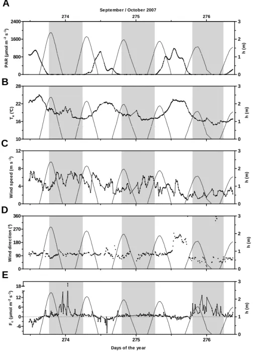
Because diurnal and tidal rhythms largely controlled the CO2 fluxes, the following results refer to the four distinct cases generated by these two cycles: emersion around low tide dur-ing the day (LT/Day), emersion at night (LT/Night), sion around high tide during the day (HT/Day) and immer-sion at night (HT/Night). The dynamics of the NEE in rela-tion to the environmental parameters are described for each EC measurement as presented in Table 1 and Figs. 3, 4, 5 and 6.

3.1 Autumn 2007 at Station 2

Over the four days of measurements in September–October 2007 at Station 2, the Arcachon flat acted as a source of CO2 to the atmosphere, with an average daily flux of 0.5 ± 0.5 g C m−2day−1 and values ranging from 0.1 to 1.0 g C m−2day−1(Table 1) . However, at shorter time scale, strong CO2 flux variations were observed with flux values ranging from −10 to 19 µmol m−2s−1, the flat shifting from sinks to source of CO2with both tidal and diurnal rhythms (Table 1, Fig. 3e). At low tide during sunny afternoons with PAR values reaching more than 1000 µmol m−2s−1 at mid-day (Fig. 3a), strong CO2uptakes (CO2sinks) were system-atically observed, as seen on Days 273 and 274, with val-ues close to 6 and 10 µmol m−2_s−1_{, respectively (Fig. 3e).} In contrast, during night time at low tide, the flat emit-ted large quantities of CO2 to the atmosphere, acting as a CO2 source (2.7 ± 3.7 µmol m−2s−1 on average, Table 1), as measured between Days 273 and 274 and between Days 275 and 276, with values largely above 10 µmol m−2s−1 (Fig. 3e). The CO2 uptake observed at LT/Day 275 was weak, reaching only 2 µmol m−2s−1, compared to that ob-served on preceding days (Fig. 3e); this change corresponded

P. Polsenaere et al.: Spatial and temporal CO2exchanges measured by Eddy Covariance 255

Table 1. Carbon dioxide fluxes (Fc)(mean ± standard deviation) measured in the Arcachon flat in September/October 2007 at Station 2 and

July 2008, September/October 2008 and April 2009 at Station 1 (see Fig. 1). Negative fluxes represent sinks of CO2and positive fluxes

represent sources of CO2to the atmosphere by convention. Averaged Fcvalues have been obtained computing the average over the whole

data set for each of the four periods. Daily Fcvalues represent the average over the averages obtained for every entire days of each period

and converted into g C m−2day−1(90 %, 92 %, 97 % and 96 % of data were used, for the deployments in autumn 2007, summer 2008, autumn 2008 and spring 2009 respectively). A PAR threshold of 20 µmol m−2s−1has been chosen to separate day and night cases and high tide cases corresponding to non-zero water heights. ∗Negative Fcdata corresponding to very short periods of low tide/night and very fast

changes in CO2fluxes in April 2009 (Days 94 and 96, Fig. 6e) were excluded from the average, as they were potentially affected by flooded

areas.

Fc Low Tide/Day Low Tide/Night High Tide/Day High Tide/Night Average Fc Daily Fc

(mean ± SD) (µmol m−2_s−1_{) (µmol m}−2_s−1_{) (µmol m}−2_s−1_{) (µmol m}−2_s−1_{) (µmol m}−2_s−1_{) (g C m}−2_day−1₎ September/October 2007 (Station 2) −1.7 ± 1.7 2.7 ± 3.7 0.4 ± 1.1 1.9 ± 2.4 0.8 ± 2.7 0.5 ± 0.5 (−10.0–0.9) (0.2–18.6) (−2.4–3.9) (−0.4–13.3) (−10.0–18.6) (0.1–1.0) July 2008 (Station 1) −0.3 ± 3.3 0.9 ± 0.8 −0.2 ± 1.4 0.7 ± 1.9 0.1 ± 1.9 0.1 ± 1.0 (−5.7–12.00) (−2.5–3.1) (−5.0–7.3) (−2.8–10.6) (−5.7–12.0) (−0.7–1.8) September/October 2008 (Station 1) −0.7 ± 2.3 0.2 ± 1.1 −0.1 ± 0.7 −0.3 ± 1.3 −0.2 ± 1.4 −0.2 ± 0.7 (−10.8–14.3) (−7.1–5.3) (−5.9–3.4) (−7.5–4.5) (−10.8–14.3) (−1.2–1.2) April 2009 (Station 1) −2.7 ± 2.0 −1.3 ± 1.4∗ −1.7 ± 1.4 −3.2 ± 2.4 −2.4 ± 2.1 −2.4 ± 0.9 (−11.7–0.6) (−6.2–1.9) (−8.7–2.6) (−13.1–0.4) (−13.1–2.6) (−4.3–−0.9)

to the occurrence of a mass of relatively hot air (approach-ing 24◦C, Fig. 3b) concomitant with a change in wind di-rection from the east-southeast (90–135◦) to south-southwest (180–225◦_{) (Fig. 3d) sectors and with a higher speed, above}

5 m s−1_{(Fig. 3c).}

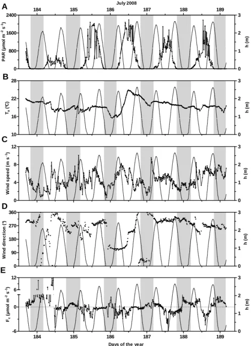
3.2 Summer 2008 at Station 1

In July 2008, at Station 1, the Arcachon flat represented a small source of CO2 to the atmosphere with a mean daily CO2 flux of 0.1 ± 1.0 g C m−2day−1, shifting from sinks to source of CO2from one day to another day (daily flux range: −0.7–1.8 g C m−2day−1, Table 1). With both diurnal and tidal cycles, the flat showed weaker CO2 exchanges than in autumn 2007 at Station 2 with CO2flux values ranging from −6 to 12 µmol m−2s−1 (Fig. 4e, Table 1). During summer 2008 at LT/Day, high CO2 uptakes were measured, reach-ing values of −5 µmol m−2s−1, as observed during Day 187 (Fig. 4e). These CO2 sinks occurred particularly during sunny days, with PAR values close to 1500 µmol m−2s−1 at midday, and were roughly synchronised with low tides (from Days 185 to 188, Fig. 4a). PAR values measured dur-ing this season showed variable but intense radiations above 2000 µmol m−2_s−1_{at midday (Days 185 and 186, Fig. 4a).} At LT/Night, CO2emissions to the atmosphere were mea-sured, with CO2flux values generally above 2 µmol m−2s−1 (Fig. 4e). At the beginning of the measurement (Days 183 and 184), this classical scheme of CO2uptake at LT/Day and CO2degassing at LT/Night was perturbed and replaced by a strong CO2source to the atmosphere, also at LT/Day, reach-ing 12 µmol m−2s−1(Fig. 4e). During this event, PAR val-ues were below 500 µmol m−2s−1at midday (Fig. 4a), and a particular mass of air coming from the south-southwest wind

sector (180–225◦) changed in speed, reaching 8 m s−1, and in direction (Fig. 4c and d).

3.3 Autumn 2008 at Station 1

Contrary to the previous measurements, in September– October 2008 at Station 1, the Arcachon flat was a sink of CO2over the twenty days, with an average daily uptake of −0.2 ± 0.7 g C m−2_day−1 _{and values ranging from −1.2 to} 1.2 g C m−2_day−1_{(Table 1). Contrasting CO}

2flux variations were also observed with natural cycles from CO2flux values of −11 to 14 µmol m−2s−1 (Fig. 5e). During this deploy-ment, medium CO2 sinks were measured at LT/Day, with values generally close to 5 µmol m−2s−1(i.e. Days 287 and 289), whereas weak CO2sources were found at LT/Night be-low 3 µmol m−2s−1(i.e. Days 286 and 288) (Fig. 5e). The PAR values were typical for the season, with some values close to 1250 µmol m−2s−1being measured at midday dur-ing sunny days. The PAR values were slightly higher than those measured during the same season in 2007 at Station 2, probably because of the presence of clouds during the four days of measurement. At Station 1, PAR values ob-served at midday decreased over the twenty days of mea-surement, from 1500 µmol m−2_s−1 _{to 1300 µmol m}−2_s−1_, i.e. at a rate of -10 µmol m−2_s−1 _{each day (Fig. 5a). As} noted in the previous measurements, reductions in CO2 in-fluxes at day and in CO2 effluxes at night were observed with immersion. Indeed, during Day 276, the CO2 flux shifted in less than one hour from −1.5 µmol m−2s−1 at LT to −0.7 µmol m−2s−1with 30 cm of water, whereas the PAR remained high and constant (Fig. 5e). During flood tide on Night 279/280, CO2 degassing decreased from 1.0 to 0.2 µmol m−2s−1in less than one hour after the tidal flat

256 P. Polsenaere et al.: Spatial and temporal CO2exchanges measured by Eddy Covariance Fig. 3 274 275 276 0 800 1600 2400 0 1 2 3 September / October 2007 P A R ( µ m o l m -2 s -1) h ( m ) 10 16 22 28 0 1 2 3 Ta ( °C ) h ( m ) 0 4 8 12 0 1 2 3 W in d s p e e d ( m s -1) h ( m ) 0 90 180 270 360 0 1 2 3 W in d d ir e c ti o n ( °) h ( m ) 274 275 276 -6 0 6 12 0 1 2 3 18 Days of the ye ar Fc ( µ m o l m -2 s -1) h ( m )

A

E

D

C

B

Fig. 3. Environmental parameters and carbon dioxide fluxes measured during the EC deployment in the Arcachon flat (St. 2) from 30

September at 11:35 to 3 October 2007 at 08:55 (GMT). (A) Photosynthetically active radiation (µmol m−2s−1)and water height (m); (B) temperature of the air (◦C); (C) wind speed (m s−1); (D) wind direction (◦) and (E) carbon dioxide fluxes (µmol m−2s−1). Negative fluxes represent sinks of CO2, and positive fluxes represent sources of CO2to the atmosphere by convention. Day 273 squares with 30 September

2007 and grey bands represent night periods. A PAR threshold of 20 µmol m−2s−1was chosen to separate day and night cases, and low tide cases correspond to zero-water heights. A specific range for Fc(E) was chosen for a better visualisation of CO2-flux variations.

immersion. Contrary to September–October 2007 at Sta-tion 2 and July 2008 at StaSta-tion 1, CO2 influxes were mea-sured at HT/Night (−0.3 ± 1.3 µmol m−2s−1on average, Ta-ble 1), as found during Night 282/283, with values reaching −7 µmol m−2_s−1_{(Fig. 5e). In addition, a strong CO}

2 emis-sion of 14 µmol m−2_s−1_{was observed at LT/Day (Day 279)} immediately after a sudden and concomitant increase in air

temperature and wind speed (Fig. 5b and c) and a switch in wind direction to the 180–225◦sector (Fig. 5d).

3.4 Spring 2009 at Station 1

In April 2009, the strongest CO2 sink was measured in the Arcachon flat, with an average daily flux of

P. Polsenaere et al.: Spatial and temporal CO2exchanges measured by Eddy Covariance 257 Fig. 4 184 185 186 187 188 189 0 800 1600 2400 0 1 2 3 July 2008 P A R ( µ m o l m -2 s -1) h ( m ) 10 16 22 28 0 1 2 3 Ta ( °C ) h ( m ) 0 4 8 12 0 1 2 3 W in d s p e e d ( m s -1) h ( m ) 0 90 180 270 360 0 1 2 3 W in d d ir e c ti o n ( °) h ( m ) 184 185 186 187 188 189 -6 0 0 1 2 3 6 12

Days of the year Fc ( µ m o l m -2 s -1) h ( m )

A

E

D

C

B

Fig. 4. Environmental parameters and carbon dioxide fluxes measured during the EC deployment in the Arcachon flat (St. 1) from 1 July at

16:40 to 7 July 2008 at 04:00 (GMT). (A) Photosynthetically active radiation PAR (µmol m−2s−1)and water height (m); (B) temperature of the air (◦C); (C) wind speed (m s−1); (D) wind direction (◦) and (E) carbon dioxide fluxes (µmol m−2s−1). Negative fluxes represent sinks of CO₂, and positive fluxes represent sources of CO₂to the atmosphere by convention. Day 183 squares with 1 July 2008 and grey bands represent night periods. A PAR threshold of 20 µmol m−2s−1was chosen to separate day and night cases, and low tide cases correspond to zero-water heights. A specific range for Fc(E) was chosen for a better visualisation of CO2flux variations.

−2.4 ± 0.9 g C m−2day−1, the flat remaining a CO2 sinks over each of the thirteen days of measurement (daily flux range: −4.3–−0.9 g C m−2day−1, Table 1). No clear pattern was observed in contrast to the previous measurements, with CO2 fluxes mostly always negative regardless of the diur-nal or the tidal phase, ranging from −13 to 3 µmol m−2s−1, the largest sinks occurring at HT during the night 96–97

(Fig. 6e). However, large sinks of CO2 also occurred at LT/Day (i.e. days 94, 95 and 103), and positive fluxes of CO2 occurred in conditions of well-established LT at night (nights 92–93, 99–100, 100–101 and 101–102) (Fig. 6e). At LT/Day during Days 95 and 96, weaker CO2influxes corresponded to cold masses of air close to 13◦C with low wind speeds near 1 m s−1and wind directions from the south-southeast (135–

258 P. Polsenaere et al.: Spatial and temporal CO2exchanges measured by Eddy Covariance

Fig. 5

Fig. 5. Environmental parameters and carbon dioxide fluxes measured during the EC deployment in the Arcachon flat (St. 1) from 25

September at 15:10 to 17 October 2008 at 01:10 (GMT). (A) Photosynthetically active radiation PAR (µmol m−2s−1)and water height (m);

(B) temperature of the air (◦C); (C) wind speed (m s−1); (D) wind direction (◦) and (E) carbon dioxide fluxes (µmol m−2s−1). Negative fluxes represent sinks of CO2, and positive fluxes represent sources of CO2to the atmosphere by convention. Day 269 squares with 25

September 2008, and grey bands represent night periods. Data between 30 September (00:10) and 2 October 2008 (07:10) could not be measured due to technical problems during the deployment. A PAR threshold of 20 µmol m−2s−1was chosen to separate day and night cases, and low tide cases correspond to zero-water heights. A specific range for Fc(E) was chosen for a better visualisation of CO2flux

variations.

180◦) (Fig. 6b, c, d and e). In contrast to the three previ-ous measurement periods, when LT/Night cases always cor-responded to CO2releases to the atmosphere due to benthic respiration, in April 2009, CO2fluxes at LT/Night were ei-ther null or negative (Table 1 and Fig. 6e). In fact, these neg-ative fluxes occurred during very short periods of LT/Night, at the end (Day 94) or at the beginning (Days 94/95 and 95/96) of the night and immediately after or before immer-sion (Fig. 6e). Negative Fcdata corresponding to very short periods of LT/Night and very fast changes in CO2fluxes were potentially affected by flooded areas and then excluded from the averages (Table 1).

3.5 Wind direction and Zostera noltii cover

Figure 7 presents the occurrence of prevailing winds per sec-tor for each period. Wind directions varied temporally ac-cording to the season and also spatially acac-cording to the station. In September–October 2007 at Station 2, the pre-vailing winds blew mostly from the southeast and east-northeast, with 60 % and 27 % of occurrence, respectively (Fig. 7a). In autumn 2008 at Station 1, no wind direction clearly prevailed; the north–northeast (0–45◦) and south– southeast (135–180◦) sectors both accounted for 20 % of the wind, and the 180–315◦sector accounted for less than 10 % (Fig. 7b). During July 2008 and April 2009 at Station 1, wind direction also changed often, but consistent prevailing winds

P. Polsenaere et al.: Spatial and temporal CO2exchanges measured by Eddy Covariance 259 Fig. 6 92 93 94 95 96 97 98 99 100 101 102 103 104 0 800 1600 2400 0 1 2 3 April 2009 P A R ( µ m o l m -2 s -1) h ( m ) 10 16 22 28 0 1 2 3 Ta ( °C ) h ( m ) 0 4 8 12 0 1 2 3 W in d s p e e d ( m s -1) h ( m ) 0 90 180 270 360 0 1 2 3 W in d d ir e c ti o n ( °) h ( m ) 92 93 94 95 96 97 98 99 100 101 102 103 104 -12 -9 -6 -3 0 3 0 1 2 3 Days of the ye ar Fc ( µ m o l m -2 s -1) h ( m )

A

E

D

C

B

Fig. 6. Environmental parameters and carbon dioxide fluxes measured during the EC deployment in the Arcachon flat (St. 1) from 1 April at

16:30 to 13 April 2009 at 22:50 (GMT). (A) Photosynthetically active radiation PAR (µmol m−2s−1)and water height (m); (B) temperature of the air (◦C); (C) wind speed (m s−1); (D) wind direction (◦) and (E) carbon dioxide fluxes (µmol m−2s−1). Negative fluxes represent sinks of CO2, and positive fluxes represent sources of CO2to the atmosphere by convention. Day 91 squares with the 1 2009 and grey bands

represent night periods. A PAR threshold of 20 µmol m−2s−1was chosen to separate day and night cases, and low tide cases correspond to zero-water heights.

occurred from the 225–315◦and the 270–360◦sectors. Con-sequently, winds from the west–northwest were mostly ob-served during both seasons, reaching more than 40 % in sum-mer 2008 and 30 % of occurrence in spring 2008 (Fig. 7c, d).

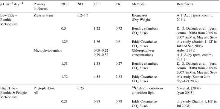
The analyses of satellite images of the tidal flat at LT/Day showed clear variations in the Zostera noltii seagrass cover according to wind directions for both stations (Table 2). In autumn 2007 at Station 2, seagrass cover was generally low (22 ± 14 % in average), ranging between 4 % and 51 % from

260 P. Polsenaere et al.: Spatial and temporal CO2exchanges measured by Eddy Covariance

Table 2. NEP values (corresponding to mean LT/Day CO2fluxes ± standard deviation) and Zostera noltii covers derived from satellite

image analyses from the Arcachon flat, at low tide during the day, according to sectors of wind direction (circle of 1000 m radius around the mast and split in 32 sectors of 11.25◦). No satellite image matching with the deployment in July 2008 at Station 1 was available.

NNE ENE ESE SSE SSW WSW WNW NNW

0–45◦ 45–90◦ 90–135◦ 135–180◦ 180–225◦ 225–270◦ 270–315◦ 315–360◦

Station 2 Autumn 2007 Zostera noltii cover (13/09/2007) 19 % 25 % 27 % 17 % 4 % 14 % 15 % 51 %

NEP (µmol m−2_s−1₎ −0.9 ± 0.7 −2.1 ± 1.4 −2.1 ± 4.4 −0.7 ± 0.6 −0.7 ± 0.7

Percentage of NEP data 4 % 61 % 7 % 21 % 7 %

Station 1 Summer 2008 NEP (µmol m−2s−1) −1.1 ± 0.9 −1.4 ± 0.3 −1.4 ± 0.6 −0.9 ± 0.9 −2.0 ± 1.4 −0.7 ± 0.2

Percentage of NEP data 11 % 6 % 14 % 18 % 47 % 4 %

Station 1 Autumn 2008 Zostera noltii cover (17/10/2008) 98 % 93 % 86 % 70 % 95 % 99 % 99 % 98 %

Zostera noltii cover (08/09/2009) 97 % 95 % 87 % 69 % 94 % 98 % 99 % 98 %

NEP (µmol m−2_s−1_{) −0.5 ± 1.5 −0.7 ± 1.3 −0.1 ± 0.9 −0.9 ± 1.0 −1.5 ± 2.6 −2.2 ± 2.0 −2.0 ± 1.1 −1.5 ± 1.2}

Percentage of NEP data 9 % 17 % 14 % 21 % 9 % 6 % 12 % 12 %

Station 1 Spring 2009 Zostera noltii cover (24/06/2009) 90 % 89 % 74 % 62 % 94 % 97 % 96 % 94 %

NEP (µmol m−2s−1) −3.8 ± 3.6 −1.0 ± 1.6 −1.6 ± 1.0 −4.5 ± 2.6 −3.0 ± 1.5 −3.1 ± 1.2

Percentage of NEP data 6 % 19 % 8 % 7 % 32 % 28 %

Fig. 7 0 20 40 60 80

Low Tide / Day Low Tide / Night High Tide / day High Tide / Night

NNW WNW WSW SSW SSE ESE ENE NNE Sept-Oct 07 P e rc e n ta g e o f o c c u re n c e ( % ) 10 20 30 40 50 NNW WNW WSW SSW SSE ESE ENE NNE July 08 P e rc e n ta g e o f o c c u re n c e ( % ) 0-45 ° 45-9 0° 90-1 35° 13 5-180° 18 0-225° 22 5-270° 27 0-315° 31 5-360° 0 10 20 30 NNW WNW WSW SSW SSE ESE ENE NNE Sept-Oct 08 Wind direction (°) P e rc e n ta g e o f o c c u re n c e ( % ) 0-45 ° 45-9 0° 90-1 35° 13 5-180° 18 0-225° 22 5-270° 27 0-315° 31 5-360° 10 20 30 40 NNW WNW WSW SSW SSE ESE ENE NNE April 09 Wind direction (°) P e rc e n ta g e o f o c c u re n c e ( % ) A C B D

Fig. 7. The wind directions during the four EC measurements in the Arcachon flat by percentage of occurrence and functions to the tidal

and diurnal rhythms (low tide/day, low tide/night, high tide/day and high tide/night). (A) 30 September to 3 October 2007 (St. 2), (b) 25 September to 17 October 2008 (St. 1), (C) 1 to 7 July 2008 (St. 1) and (D) 1 to 13 April 2009 (St. 1).

the south–southwest and east–southeast wind sectors, respec-tively (Table 2). A significant difference in the seagrass cover was computed between wind sectors 146.25–247.5◦/78.5– 146.25◦ with 4 ± 3 % (0–9 %) and 24 ± 13 % (7–37 %) re-spectively (p = 0.0027). In autumn 2008 at Station 1, higher

Zostera noltii covers were measured than during the same

season in 2007 at Station 2 (92 ± 10 % in average), with

val-ues ranging between 70 % (south-southeast) and 99 % (west-northwest) (Table 2). Similarly, a clear Zostera noltii sea-grass cover variation was observed between wind sectors 11.25–168.75◦and 168.75–360◦with 86 ± 13 % (55–100 %) and 96 ± 5 % (80–100 %) respectively (p = 0.0012). The next year, in autumn 2009, exactly the same percentage of

Zostera noltii cover was observed (92 ± 10 % in average),

P. Polsenaere et al.: Spatial and temporal CO2exchanges measured by Eddy Covariance 261

between 69 and 99 % (Table 2). In regards to the spring de-ployment at Station 1 in 2009, no matching satellite image was available; the analysis of the image recorded on April 2010 (14/04), the year after the EC deployment, showed a very low seagrass cover, below 5 %, regardless of wind di-rection (data not shown). The image recorded on 24 June 2009, obtained ten weeks after this spring EC deployment, showed slightly lower seagrass cover than in late summer– autumn (87 ± 13 % in average, range: 62–97 %, Table 2) but higher than that measured previously, in early spring 2010. A variation in the seagrass cover was also observed between wind sectors 135–247.5◦and 101.25–135◦/247.5–360◦, with 80 ± 22 % (36–99 %) and 91 ± 7 % (75–97 %) respectively (p = 0.823).

4 Discussion

4.1 Spatial and temporal variations of NEE in relation to NEP of the Arcachon flat

4.1.1 Diurnal and tidal changes in NEE at the different seasons

Throughout the diurnal and tidal cycles, variations in NEE were large, with the flat often rapidly shifting from source to sink. For instance, at Station 1 in July 2008 on Day 184 and daytime, NEE rapidly dropped from 12.0 µmol m−2s−1 at low tide to −5.0 µmol m−2s−1as soon as the water sub-merged the flat. Inversely, at night, between Days 187 and 188, the CO2flux was −0.8 µmol m−2s−1at the end of the immersion and rose to 3.0 µmol m−2_s−1_{at the beginning of} the emersion (Fig. 4e). There are a number of processes that can induce these rapid changes in NEE, including benthic and planktonic GPP and CR, advection with water move-ments and air-water gas exchange. Although in the inter-tidal Wadden Sea, Zemmelink et al. (2009) found little de-pendency of CO2fluxes on the tide, this was not the case in the Arcachon flat. The effect of rising tide on CO2exchange was first reported by Houghton and Woodwell (1980) in a salt marsh. Kathilankal et al. (2008) reported a 46 % reduc-tion in CO2uptake during emersion. In these salt marsh sys-tems, part of the vegetation remains emerged even at high tide. In intertidal systems like Arcachon or the Wadden Sea, at low tide, benthic GPP and CR are theoretically the two main drivers of NEE. When the tide rises over the flat, benthic and planktonic communities contribute to GPP and CR, but their effect on NEE may not be immediate because water-air gas exchange is slow in comparison with the dura-tion of the immersion. For instance, for typical condidura-tions in coastal systems and a gas-transfer velocity of 10 cm h−1, it takes 3.5 h for pCO2 to decrease from 600 to 500 ppmv with gas exchange, which corresponds to a CO2 flux of ∼1.2 µmol m−2s−1, comparable to what we observed here. Consequently, a negative water–air gradient can be created,

for instance by phytoplankton at the mouth of the flat at low tide, then these CO2-undersaturated waters can enter with the flood tide. This would generate a negative NEE in the flat at high tide, that would not result from the in situ NEP. In-versely, intense benthic and planktonic CR at high tide in the flat would not necessarily immediately generate an equiva-lent degassing of CO2to the atmosphere, with some of the CO2remaining in solution and being exported laterally with the subsequent ebb tide. Such CO2 outwelling from inter-tidal systems to adjacent creeks and bays has been observed in many tidal wetlands (Cai et al., 2003; Wang and Cai, 2004; Borges et al., 2003).

The September 2007 measurements at Station 2 in the in-ner part of the flat provide a first and relatively simple scheme for conceptualising NEE dynamics in relation to NEP at the different phases of the day and the tide. During this exper-iment, we observed strong CO2 uptake at LT/Day but CO2 degassing during all other cases (Fig. 3e, Table 1). This sug-gests that at LT/Day, the tidal flat was autotrophic, whereas it was heterotrophic during the night and during immersion. In addition, CO2degassing at LT/Night and HT/Night was sig-nificantly higher (p < 0.05) than at HT/Day, which suggests that in the daytime during immersion, benthic and planktonic GPP significantly reduce CO2degassing from waters. Ben-thic GPP by microphytobenthos is controlled by light avail-ability (Parsons et al., 1984) and is believed to be light lim-ited during immersion. At Station 2, where the Zostera noltii cover was particularly low, microphytobenthos, could signif-icantly be resuspended and contribute to planktonic GPP at the beginning of the flood tide (Guarini, 1998).

At Station 1, in the centre of the flat, patterns of CO2fluxes were fundamentally different, as uptake of atmospheric CO2 were also observed during the immersion. This occurred ing the day at the three periods of measurements and also dur-ing the night in September 2008 and in April 2009. In con-trast, in July 2008, the flat was a source of CO2at HT/Night, being a sink at HT/Day (Table 1). Negative NEE during HT/Night demonstrates the impact of planktonic GPP at the outlet of the flat, followed by advection of CO2-depleted wa-ter masses with the flood tide. Indeed, the channel and sub-tidal areas of the flat are the sites of development of phy-toplankton blooms with high primary production rates, par-ticularly in early spring (Gl´e et al., 2007, 2008). In April 2009, the uptake of atmospheric CO2 during immersion at Station 1 was nearly two times higher at night time than at daytime (Table 1). This suggests that the CO2depletion of the waters may have occurred at daytime a few hours before, precisely when the water masses were at the mouth of the flat. On the contrary, the water present at daytime over the tidal flat absorbed less atmospheric CO2, as it was present at the outlet of the flat around night time; this also suggests that during this spring period, GPP during immersion was lower in the flat than outside of the flat, consistent with results of Gl´e et al. (2007) who showed planktonic primary production always higher in external waters.

262 P. Polsenaere et al.: Spatial and temporal CO2exchanges measured by Eddy Covariance

In July and September 2008, NEE during immersion at Station 1 showed different patterns. In September, NEE was slightly negative (∼−0.2 µmol m−2_s−1_{; Table 1) at both} HT/Day and HT/Night, suggesting, as in April 2009, a pre-dominant role of advection of CO2-depleted waters from the mouth of the flat. In contrast, in July 2008, the water in the flat was a sink of CO2at daytime but a source of CO2at night (Table 1), meaning that advection phenomena were probably less important than metabolic processes inside the flat itself, by both planktonic and benthic communities. CO2 uptake at LT/Day measured by EC was systematically reduced at HT/Day during the four deployments (Figs. 3, 4, 5, 6e and Table 1). This was especially true in the summer and au-tumn seasons in 2008 at Station 1, when the Zostera noltii cover was maximal. This could be due to lower photosyn-thetic activity of primary producers due to light limitation in the presence of water, or to a delay in water-air gas equilibra-tion, as previously discussed. Little is known about seagrass metabolism in coastal flats, especially on NPP and photosyn-thetic efficiency during air-exposed versus immersed condi-tions (Silva et al., 2005, 2008; Abril, 2009; Silva and San-tos, 2009; Clavier et al., 2011). Using benthic chambers, Clavier et al. (2011) observed in the Banc d’Arguin (Mau-ritania) carbon fluxes by Zostera noltii beds greater under water than when exposed to air. Another key factor for CO2 uptake by air-exposed Zostera noltii is the leaf water con-tent (Leuschner et al., 1998). In tidal flats, the existence of depressions in the sediment at low tide can retain enough amount of water to maintain leaf hydration, and allow high photosynthetic rates of the seagrass and rapid air-water CO2 diffusion (Silva et al., 2005). Because CO2 diffuses much slowly through the water-air interface than through air, the carbon uptake we observed during tidal flooding in the flat is probably more related to the initial pCO2of waters entering the flat, than to the in situ photosynthetic activity of Zostera

noltii underwater.

Finally, another type of physical processes was driving CO2 fluxes in the flat, and resulted in very strong CO2 de-gassing to the atmosphere at LT/Day at Station 1, in July 2008 on Day 184 (Fig. 4e), and in September–October 2008 on Day 279 (Fig. 5e). Such singular CO2degassing was too high and rapid to be explained by biological respiration, and was obviously caused by destocking processes linked to the onset of atmospheric turbulence (high wind speeds). These destocking events were not related to the tide; they occurred during the emersion in the morning and were concomitant with sudden changes in wind direction.

4.1.2 Relationship between low tide CO2fluxes and the

distribution of Zostera noltii meadows

CO2fluxes between the Arcachon flat at low tide and the at-mosphere showed important spatial and temporal variations. Significant spatial and temporal differences in Zostera noltii cover were also observed from satellite images (Table 2).

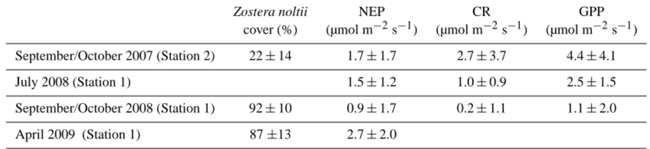
For the low tide conditions, we can assume that benthic CR was equivalent to NEE at night (Rocha and Goulden, 2008), and benthic NEP was equivalent to NEE averaged over the daytime. GPP at low tide can be calculated as the NEE at night minus the NEE during the day, as presented in Table 3. In autumn 2007 at Station 2 with a low Zostera noltii density, a particularly high GPP of 4.4 ± 4.1 µmol m−2s−1 was calculated, the CR showing the highest value, with 2.7 ± 3.7 µmol m−2s−1 (Table 3). In contrast, in autumn 2008 at Station 1 with a high Zostera noltii density, a slightly low GPP of 1.1 ± 2.0 µmol m−2s−1was found, the CR be-ing only 0.2 ± 1.1 µmol m−2s−1(Table 3). At both stations, rapid changes in CO2 fluxes (NEP) were observed in rela-tion to wind direcrela-tion and seagrass cover; the most nega-tive (highest NEP) and the less neganega-tive (lowest NEP) CO2 fluxes matched the highest and the lowest seagrass cover, respectively (Table 2). For instance, in September 2007 at Station 2, mean fluxes from the 78.75–90◦ _{wind sector}

with a seagrass cover of 24 ± 13 % were −2.2 ± 1.8 whereas those from the 146.25–247.5◦ sector with a 4 ± 3 % cover were −0.6 ± 0.6 µmol m−2s−1. Such correspondence be-tween NEP at low tide and seagrass cover was observed at all stations and seasons (Table 2). These results indicate that

Zostera noltii greatly contribute to the NEP in the central part

of the flat, from spring to autumn. In areas where the Zostera

noltii cover remains low all year round like the inner part

of the flat (Plus et al., 2010), microphytobenthos communi-ties potentially play a large role in the benthic metabolism and CO2 fluxes at low tide. Indeed, at Station 2, the av-erage computed NEP was slightly higher than at Station 1, but CR and thus the GPP were much higher than at Station 1 (Table 3). Such high GPP by microphytobenthos at low tide has been reported in many temperate intertidal mudflats (Guarini, 1998; Spilmont et al., 2006). These high GPP val-ues are associated with high CR valval-ues at night due to het-erotrophic bacteria (Hubas et al., 2006) and consistent with our observation with the EC at Station 2 (Table 3). In par-ticular, Goto et al. (2001) have shown that benthic bacteria can utilize exudates from microphytobenthos. Also, high CR rates can be accounted for by the intense grazing of meio-fauna and macromeio-fauna on microphytobenthos, the latter being easily and rapidly transferred toward superior benthic het-erotrophic components (Middelburg et al., 2000; Spilmont et al., 2006). Our EC data also reveal a clear seasonal cycle at Station 1, with a decrease of NEP from April through July to September (Table 3), a temporal pattern very consistent with the growing cycle of Zostera noltii (Auby and Labourg, 1996). There were probably also some changes in the contri-bution of the benthic primary producers (Zostera noltii, as-sociated epiphytes and benthic microalgae) over the course of the year, that could occur in a relatively constant rate of production at the community scale, as shown by Ouisse et al. (2010) using static chambers.

GPP and CR calculations could not be performed from the EC data obtained in April 2009 (Station 1); CO2fluxes

P. Polsenaere et al.: Spatial and temporal CO2exchanges measured by Eddy Covariance 263

Table 3. Comparison of NEP components at low tide for the autumn season at the two stations and in summer at Station 1. NEP was assumed

as NEE at low tide during daytime, CR was assumed as NEE at low tide during the night, and GPP was assumed as the sum of NEP and CR. Notice that Fcvalues obtained in July 2008 during the beginning of the experiment (Days 183, 184) and in September–October 2008 (Day

279) have been discarded for calculations, representing destocking but not biological degassing by respiration (Figs. 5f and 6f). The GPP and CR calculations for the spring 2009 period at Station 1 were not possible because of the slight negative averaged flux value obtained at Low Tide/Night (see discussion). Zostera noltii covers for the April 2009 flux data are derived from a SPOT image from ten weeks later (26 June 2009) and are thus probably much higher than during the flux measurements.

Zostera noltii NEP CR GPP

cover (%) (µmol m−2s−1) (µmol m−2s−1) (µmol m−2s−1) September/October 2007 (Station 2) 22 ± 14 1.7 ± 1.7 2.7 ± 3.7 4.4 ± 4.1 July 2008 (Station 1) 1.5 ± 1.2 1.0 ± 0.9 2.5 ± 1.5 September/October 2008 (Station 1) 92 ± 10 0.9 ± 1.7 0.2 ± 1.1 1.1 ± 2.0 April 2009 (Station 1) 87 ±13 2.7 ± 2.0

over the mudflat were null or slightly negative at LT/Night and could not be attributed to benthic CR. In the unvege-tated tidal flat of the Wadden Sea at the same season, Zem-melink et al. (2009) reported null and negative CO2 fluxes with both EC and chamber techniques. Several processes could partly explain these fluxes in the Arcachon mudflat during this season, when the Zostera noltii density was low and microphytobenthic also contributed to NEP. First, micro-phytobenthic cells can migrate down to deeper layers of the sediment at night as protection against grazing by deposit-feeders (Blanchard et al., 2001); thus, respiration would not release CO2to the atmosphere but deeper into the sediments. Second, CO2 generated by benthic respiration could be al-most entirely involved in the dissolution of carbonate shells and not released to the atmosphere, as occurred for instance in a Mediterranean seagrass meadow (Posidonia oceanica) in winter (Barr´on et al., 2006). The Arcachon flat repre-sents an important stock of carbonates of about 120 Mt of several shellfish species as Crassostrea gigas contributing to 95 % (D. M. X. De Montaudouin, personal communication, 2011). From the end of the reproduction season (November) to the spat removing in spring, juvenile bivalves are particu-larly sensitive to dissolution-induced mortalities as shown by Green et al. (2004) in laboratory on the juvenile bivalve

Mer-cenaria merMer-cenaria. Thus, CaCO3dissolution could occur in wet mud sediments in presence of such shellfishes patchy distributed on the tidal flat.

To complete our analysis on the controlling factors of CO2 fluxes at LT/Day, NEE-PAR relations ranked by wind direc-tion and Zostera noltii cover were analysed (Table 4). Sig-nificant (p < 0.01) negative or positive correlations were ob-tained at Station 1 (Table 4). Negative correlations occurred in areas with a high Zostera noltii cover (>93 %), whereas positive correlations occurred in areas with lower Zostera

noltii cover (<83 %). Note that for the April 2009 period,

the Zostera noltii cover was obtained from a SPOT image

from 24 June 2009, so the real cover during the measure-ments is probably much lower. Nevertheless, the first two sectors in Table 4 for this season have much higher seagrass covers than the last two sectors. As Zostera noltii growths in well-defined areas from spring to summer (Plus et al., 2010), differences in NEE-PAR correlations are indeed re-lated to large differences in the seagrass cover in spring, during the measurements. These negative correlations be-tween NEE and PAR (or positive correlations bebe-tween NEP and the intensity of available light) reveal an optimal adapta-tion of the plants to the environmental condiadapta-tions created by the solar radiation, such as temperature, humidity and light. Similar negative correlations have been observed with EC by Morison et al. (2000) for the C4aquatic grass Echinochloa polystachya of the Amazon and by Kathilankal et al. (2008)

for the Spartina alterniflora in a salt marsh on the eastern coast of Virginia. Using static chambers, Silva et al. (2005) obtained the same results for Zostera noltii meadows in the intertidal flats of the Ria Formosa flat in Portugal. The fact that these negative correlations occur in areas with the high-est Zostera noltii cover confirms that the seagrass in the Ar-cachon flat grows in optimal light condition and that its pho-tosynthetic activity dominates the CO2 uptake at low tide where the plant prevails. To the contrary, the three sig-nificant positive linear regressions observed in areas with lower Zostera noltii cover (Table 4) suggests another dom-inant metabolism that responses differently to the light in-tensity. In intertidal mudflats dominated by microphytoben-thos, negative correlations between CO2 fluxes and irradi-ance have been systematically observed with static chambers (Guarini, 1998; Spilmont et al., 2006; Mign´e et al., 2007). There was no significant correlation between NEE and air temperature during these three measurements periods, which precludes the hypothesis of a stimulation of CR by surface heating. Photoinhibition of photosynthesis by microphyto-benthos may occur, but this mechanism has been observed