Forecasting world and regional air traffic in the
mid-term (2025): An econometric analysis of air traffic
determinants using dynamic panel-data models
∗
Benoît Chèze
†‡, Julien Chevallier
§, and Pascal Gastineau
¶January 31, 2011
Abstract
This article proposes an econometric analysis of the demand for mobility in the avi-ation sector. The role played by different variables (GDP, jet-fuel prices, exogenous shocks, market maturity) on air traffic is estimated using dynamic panel-data modeling. GDP appears to have a positive influence on air traffic, whereas Jet-Fuel prices have a non-linear effect on air traffic. Our analysis shows that the magnitude of the influence of these air traffic determinants differs widely among regions. Then, we use our model to predict the evolution of air traffic until 2025. According to our main scenario, air traffic should be multiplied by a factor of two between 2008 and 2025 at the world level, cor-responding to a yearly average growth rate of 4.7% (ranging from 3% in North America to 8% in China, at the regional level) expressed in RTK.
Keywords: Air Traffic Determinants; Dynamic Panel Data; Forecasting. JEL Classification Numbers: C01; C32; Q43; Q54
∗The research leading to these results has received funding from the European Community’s Seventh
Framework Programme (FP7/2007-2013) under grant agreement ACP7-GA-213266 (Alfa–Bird). The authors are grateful to Laurie Starck (IFP Energies nouvelles (IFPEN)) for her valuable help. The authors also wish to thank for their helpful comments Laurent Meunier (ADEME) and from the IFPEN: Emilie Bertout, Nicolas Jeuland, Pierre Marion, Axel Pierru, Valérie Saint-Antonin, Stéphane Tchung-Ming and Simon Vinot. The usual disclaimer applies.
†Corresponding author. IFP Energies nouvelles, 1-4 avenue de Bois-Préau, 92852 Rueil-Malmaison, France.
‡EconomiX–CNRS, Université Paris Ouest, Nanterre–La Défense.
§Université Paris Dauphine (CGEMP/LEDa) & EconomiX–CNRS; [email protected]. ¶IFSTTAR; [email protected].
1
Introduction
According to the International Civil Aviation Organization (ICAO)1, air traffic is characterized by mean annual growth rates comprised between 5% and 6% since the middle of the 1980s (ICAO, 2007). This growth, strictly superior to that of other economic sectors, is expected to sustain in the coming years. The main actors in the aeronautical industry anticipate for instance the same sustained growth rate for the next twenty years (Airbus, 2007; Boeing, 2009). If these projections were to come true, they would imply a multiplication by a factor of two of air traffic at the worldwide level by 2025.
This strong and rapid growth of air transport is arguably a factor of economic growth, facilitating international exchanges (among others). Yet, in a scarce energy resources context, this development may appear problematic during the 21st century, leading to an increased interest for policy makers2. The classical example is the inclusion of the aviation sector in the
EU Emissions Trading Scheme (EU ETS) in January 20123.
Hence, forecasting and modeling air transport demand has become a central issue for public policy, that this article aims at pursuing. To understand the evolution of this demand, we must start by studying the fundamentals of this transportation means. This first task is developed by using econometric methods. Then, we perform various forecasts for air traffic in the mid-term (2025), at the world and regional levels. These forecasts are derived from the prior modelling and estimation of the relationship between air transport and its main determinants.
To perform air traffic forecasts, the relationship between air traffic and its main fundamen-tals is first estimated econometrically over around thirty years (1980-2007). Several factors of air transport are therefore identified. This analysis supports an interpretation of world air traffic growth in which GDP and Jet-Fuel prices play a central role. The former variable has a positive influence on air traffic, whereas the latter variable is expected to have a neg-ative influence. Based on panel-data econometric modelling, we show that the sensitivity of air transport differs depending on the degree of maturity of the market under consideration. Then, various scenarii are proposed concerning the evolution of these fundamentals. Once the econometric relationship has been estimated and the scenarii have been defined, we obtain
1
The ICAO is a body from the United Nations created in 1947 to standardize international security and navigation rules in the air transport sector.
2
See among others on this topic: ECI (2006), IEA (2009a, 2009b, 2009c), IPCC (1999, 2007a, 2007b, 2007c) and RCEP (2002).
3
The amending Directive 2003/87/EC highlights that ‘emissions from all flights arriving at and departing from Community aerodromes should be included’.
various trajectories for the evolution of air traffic. Depending on the assumptions made on the evolution of air traffic drivers, we obtain different air traffic projections. This modelling, and the associated forecasts, are applied to eight geographical zones4 and at the world level (i.e. the sum of the eight regions) by specifying a dynamic model on panel data. According to our main air traffic forecast scenario, at the world level, air traffic (expressed in RTK5) should increase with a yearly average growth rate of 4.7%. These air traffic forecasts differ from one region to another. At the regional level, yearly average growth rates range from 3 % in North America to 8.2 % in China.
The paper is organized as follows. Section 2 introduces some historical trends. Section 3 reports and discusses the econometric results. Section 4 presents different air traffic scenarii. Section 5 briefly concludes.
2
Evolution of air traffic
This section details the evolution of air transport from 1980 to 2007 at the worldwide level and for eight regions. It highlights the regional heterogeneity, which has important consequences in terms of forecasting air traffic.
2.1
Data
Air Traffic data from 1980 to 2007 have been obtained from the ICAO6. This specialized
agency of the United Nations provides the most complete air traffic database7: international and domestic, passenger and freight traffic (both for scheduled and non-scheduled flights).
The database used is entitled ‘Commercial Air Carriers - Traffic’. It contains, on annual basis, operational, traffic and capacity statistics of both international and domestic scheduled airlines, as well as non-scheduled operators. Where applicable, the data are for all services (passenger, freight and mail) with separate figures for domestic and international services,
4
Air traffic forecasts are computed for the following regions: Central and North America, Latin America, Europe, Russia and CIS (Commonwealth of Independent States), Africa, the Middle East, Asian countries and Oceania (except China). China is the eighth region. We choose to focus on that specific region due to its steady economic growth.
5
Revenue Ton Kilometer (RTK) is defined as one ton of load (passengers and/or cargo) carried for one kilometer.
6
http://www.icaodata.com
7
Note the International Air Transport Association (IATA), which represents about 230 airlines comprising 93% of scheduled international air traffic, also provides Air Traffic data, but this source is less detailed to our best knowledge.
for scheduled and non-scheduled services, and for all-freight services8. The main interest of this database consists in providing data by country, and not by pre-aggregated regions. Thus, it allows to recompose any kind of regions depending on any scenarii. Within the database by country, statistics are provided for airlines registered in a given country on a yearly basis9. Another advantage lies in the possibility to account for freight vs. passenger, and for domestic vs. international air traffic within each zone. There exists however one limitation with the use of such data for international air traffic. When re-aggregating the data by zone, one considers that the airline which declared the flights as ‘international air traffic’ has not registered international flights outside the country within which it is registered, and thus outside of the region within which it has been re-aggregated.
Cargo traffic is measured in Revenue Ton Kilometers (RTK) whereas passenger traffic is
expressed both in Revenue Passenger Kilometers (RPK10) and RTK.
Unless otherwise indicated, all descriptive statistics presented below are valid during 1980– 2007. Note that air traffic statistics are not available before 1983 for Russia and CIS. In order to account for this gap, we present the descriptive statistics only during 1983-2006.
The decomposition in geographical zones follows a classical representation. Thus, we ob-tain air traffic for eight distinct regions (Central and North America, Latin America, Europe, Russia and CIS, Africa, the Middle East, China, Asian countries and Oceania), and on a worldwide basis (computed as the sum of the eight regions).
The following sections present in more details the air traffic database from the ICAO.
2.2
Evolution of air traffic during 1980–2007
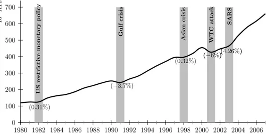
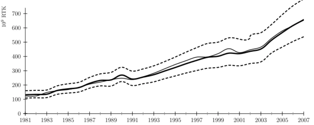
Figure 1 shows the evolution of world air traffic from 1980 to 2007.
Two major remarks may be inferred from this graph. First, it emphasizes the strong increase of this sector, with a variation growth of +340% during the period. Second, the aviation sector - cyclical in nature - has encountered some specific shocks (represented with gray solid bars) that all had downward impacts on the demand for air travel (Mason, 2005). Figures in brackets represent the variation of activity of the aviation sector during these events. The terrorist attacks in New York and Washington had a major impact on the airline industry (Alderighi and Cento, 2004; Ito and Lee, 2005). These attacks caused many travelers
8
These data are not provided on air routes basis.
9
With such statistics, air traffic data of a given airline cannot be provided in two different tables. Thus, it avoids the problem of double-counting.
10
Revenue Passenger Kilometers (RPK) is a measure of the volume of passengers carried by an airline. A revenue passenger kilometer is flown when a revenue passenger is carried one kilometer.
0 100 200 300 400 500 600 700 1980 1982 1984 1986 1988 1990 1992 1994 1996 1998 2000 2002 2004 2006 U S r e str ic ti v e m o ne ta r y p o li c y (0.31%) G ul f c r isi s (−3.7%) A si a n c r isi s (0.32%) W T C a tta c k (−6%) SA R S (4.26%) 10 9R T K
Note: Figures into brackets indicate air traffic growth rates during specific events.
Figure 1: Evolution of world air traffic (1980-2007) expressed in RTK (billions). Source: Authors, from ICAO data.
to reduce or avoid air travel and resulted in a transitory, negative demand shock in addition to an ongoing negative demand shift (Inglada and Rey, 2004; Guzhva and Pagiavlas, 2004; Njegovan, 2006a). The recovery patterns clearly vary across countries and regions (Gillen and Lall, 2003). Airlines were also affected by macroeconomic shocks such as the Asian financial crisis, the SARS (Severe Acute Respiratory Syndrome) and the Gulf Wars.
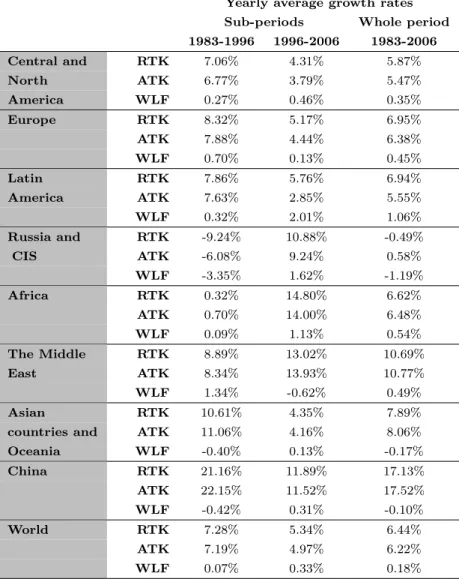
Table 1 provides air traffic statistics, expressed in levels, for each zone and the world. Data are presented within two sub-periods: 1983–1996 and 1996–2006. Note that air traffic data are expressed in two different units: RTK and ATK11. RTK measures actual air traffic, whereas ATK is a unit to measure the capacity of an aircraft/airline. The link between these two units is the Weight Load Factor (WLF): RT K = W LF ×AT K with WLF the percentage of an aircraft’s available ton effectively occupied during a flight. Then, if airline companies fill their aircrafts at the maximum available load (W LF = 100%), RTK is strictly equal to ATK. Because airlines never fully fill their aircrafts, ATK > RTK.
Note that in this article air traffic is measured in ton kilometer (as opposed to passenger kilometer). This explains why there is typically a 10 percentage points difference between the WLF value presented in Table 1 and the usual WLF as read in the literature which are rather expressed in passenger kilometer (thereafter called Passenger Load Factors (PLF)).
As a stylized fact, Table 1 shows that during the whole period airline companies’ WLF
11
Available Ton Kilometer (ATK) is a measure of an airline’s total capacity (both passenger and cargo). It is the capacity in tons multiplied by the number of kilometers flown.
Yearly average growth rates Sub-periods Whole period 1983-1996 1996-2006 1983-2006 Central and RTK 7.06% 4.31% 5.87% North ATK 6.77% 3.79% 5.47% America WLF 0.27% 0.46% 0.35% Europe RTK 8.32% 5.17% 6.95% ATK 7.88% 4.44% 6.38% WLF 0.70% 0.13% 0.45% Latin RTK 7.86% 5.76% 6.94% America ATK 7.63% 2.85% 5.55% WLF 0.32% 2.01% 1.06% Russia and RTK -9.24% 10.88% -0.49% CIS ATK -6.08% 9.24% 0.58% WLF -3.35% 1.62% -1.19% Africa RTK 0.32% 14.80% 6.62% ATK 0.70% 14.00% 6.48% WLF 0.09% 1.13% 0.54% The Middle RTK 8.89% 13.02% 10.69% East ATK 8.34% 13.93% 10.77% WLF 1.34% -0.62% 0.49% Asian RTK 10.61% 4.35% 7.89%
countries and ATK 11.06% 4.16% 8.06%
Oceania WLF -0.40% 0.13% -0.17% China RTK 21.16% 11.89% 17.13% ATK 22.15% 11.52% 17.52% WLF -0.42% 0.31% -0.10% World RTK 7.28% 5.34% 6.44% ATK 7.19% 4.97% 6.22% WLF 0.07% 0.33% 0.18%
Table 1: Yearly average growth rates of air traffic (expressed in RTK and ATK (billions)) and Weight Load Factor for each zone during 1983-2006. Source: Authors, from ICAO and IEA data.
values have rather increased. For instance, at the world level, WLF mean yearly growth rates for the first sub-period are equal to 0.07% – thus registering a constant WLF – and to 0.65% during the second sub-period – thus registering a steady WLF increase of 0.6% per year. This evolution is common to most regions, except in China, Asian countries and Oceanian regions where the mean yearly growth rate of the WLF is negative during the first sub-period. Globally, we still notice the stylized fact that on average aircrafts are less filled during the first sub-period compared to the second one.
Yearly mean growth rates are provided in the last three columns. World air traffic (ex-pressed in RTK) has registered a yearly mean growth rate of 6.4% on the whole period.
This mean growth rate is higher during the first sub-period (7.28%) than during the second sub-period (5.34%).
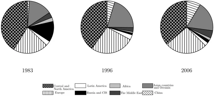
Various yearly mean growth rates may be observed within each zone (Table 1), which ex-plains the evolution of each zone’s weight in total air traffic as depicted in Figure 2. The share of the USA and Europe in total air traffic represents around two thirds. This share appears stable over the period (62.93% in 1983 compared to 62.61% in 2006). It is due to the fact that the share of the USA has decreased (with a mean variation growth of -11.90%), while the share of Europe has increased (with a mean variation growth of +21.25%) during the whole period. With its strong economic growth and large population size, China is becoming a major player in air transportation (Shaw et al., 2009). The share of China in total air traffic has skyrocketted during the second sub-period, going from 4.74% in 1996 to 8.57% in 2006. Its mean variation rate represents +80% for a yearly mean growth rate of +11.89% (Table 1). In order to diversify their traditionnally oil- and gas- dependent economies, some Middle Eastern countries (such as the United Arab Emirates and Qatar) pursue substantial invest-ments into their aviation sector (Vespermann et al., 2008). The share of the Middle East in total air traffic represents 4.66% in 2006. Africa plays a minor role in the global air transport pattern (Mutambirwa and Turton, 2000). Figure 3 offers an alternative view of this evolution.
1983 1996 2006
Central and Europe
Latin America Russia and CIS
North America Africa
The Middle East
Asian countries and Oceania
China
Figure 2: World repartition by zone in 1983, 1996 and 2006 of air traffic (expressed in RTK). Source: Authors, from ICAO data.
Besides, the ICAO provides highly detailed data for freight, passengers, domestic and international air traffic. It allows us to present the evolution of air traffic for each zone in
different ways: freight vs. passengers, and domestic vs. international.
Passengers’ traffic predominates at the world level with a share of 91.93% in 1983 and 85.07% in 2007. The share of freight traffic has almost doubled. This comment applies for most cases, except in Russia and CIS, Africa, Central and North America. The repartition is globally more in favor of passengers’ traffic in the two former zones. In North America however, freight traffic has more increased than in the other zones, going from 9.12% in 1983 to 18.49% in 2007.
At the world level, the repartition of air traffic between international and domestic has always been more favorable to international air traffic. This share has greatly increased, going from 55.33% in 1983 to 70.77% in 2006, meaning that globally international air traffic has more grown than domestic air traffic. At the regional level, this share is even more in favor of international air traffic (around 95% in 2006 in Europe for instance). The world statistic appears biased by the repartition between international (43.84% in 2006) vs domestic (56.16% in 2006) air traffic in Central and North America. This region is the only one to feature a repartition more favorable to domestic air traffic, even if international air traffic has increased during the period (32.79% in 1983, 43.84% in 2006). This analysis confirms the role played by (i) the domestic market for air transport in the USA; and (ii) the weight of the North American zone in total air traffic (about 36% in 2006 according to Figure 2). Next, we carry out the air traffic econometric analysis.
3
Air traffic econometric analysis
Gravity models appear to be the most intuitive modeling, since it represents a way to model journeys by following specific routes (Jorge-Calderon, 1997; Graham, 1999; Wojahn, 2001; Becken, 2002; Swan, 2002; Bhadra, 2003; Jovicic and Hansen, 2003; Njegovan, 2006b; Wei and Hansen, 2006; Grosche et al., 2007; Bhadra and Kee, 2008; DfT, 2009). However, this approach is not adopted here for different reasons. The first reason is linked to data access limitations. Recall that the ICAO provides air traffic by routes only for international scheduled air traffic (not for domestic air traffic)12. Second, even if all routes data could be accessed, there would remain the problem of re-aggregating journeys by route which can be extremely
12
When forecasting air traffic at the worldwide level, this data limitation generates some incoherence in the methodology used: international air traffic may be modeled by route, while domestic air transport cannot. This limitation involves to use another type of dataset.
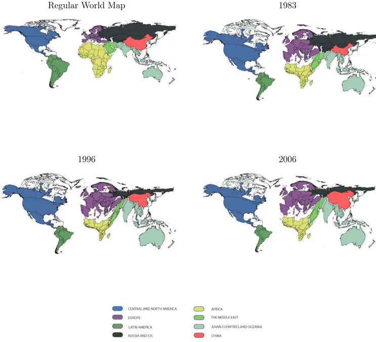
Regular World Map 1983
1996 2006
Note: These cartograms size the geographical zones according to their relative weight in world air traffic (expressed in RTK), offering an alternative view to a regular map of their evolution from 1983 to 2006. Maps generated using ScapeToad.
Figure 3: An alternative view of the evolution of the share of each region’s air traffic in 1983, 1996 and 2006.
time consuming. Thus, if gravity models appear to be more appropriate at first glance, they do not necessarily fit well when one wants to model Air traffic at the worldwide level.
For all these reasons, a more parsimonious approach is adopted here by modeling air traffic demand based on panel-data econometric techniques. Before presenting the estimates, the potential explanatory variables of air traffic are detailed (Gately, 1988; Greene, 1992, 1996, 2004; Vedantham and Oppenheimer, 1998; Lee et al., 2001, 2004, 2009; Eyers et al., 2004; Riddington, 2006).
3.1
Analysis of potential determinants
This section presents the main drivers of air traffic demand. Previous literature identifies broadly three categories of air traffic drivers. The first type is represented by GDP growth rates, the second deals with the ticket price, and the third concerns exogenous shocks. Besides, the magnitude of the influence of these air traffic determinants depends on the market maturity of each region.
3.1.1 GDP
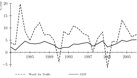
Figure 4 presents the respective growth rates of world GDP vs. world air traffic (measured in RTK). 0 5 10 15 20 −5 1985 1989 1993 1997 2001 2005 % / y ea r
World Air Traffic GDP
Figure 4: Comparison of GDP (solid line) and world air traffic (dashed line) growth rates during 1981-2007. Source: Authors, from ICAO and Thomson Financial Datastream Data.
Figure 4 confirms that world air traffic has been increasing at 6.4% on average during 1980-2006 (see Table 1), while world’s GDP growth rates have a mean value of 3.3%. When comparing GDP growth rates and the rate of growth of the aviation sector, one may conclude
that the aviation sector is characterized by a dynamic growth compared to other sectors in the economy. Moreover, we notice a high variability in the range of world’s air traffic growth rates, going from +20% in 1983 to -6% in 2001.
3.1.2 Ticket prices
Dresner (2006) and Graham and Shaw (2008) show that there exists a negative elasticity between ticket prices and air traffic: the higher ticket prices, the lower the demand for flights. More particularly, Dresner (2006) indicates that leisure passengers display higher elasticities of demand and lower valuations for travel time compared to business travelers13. According to Graham and Shaw (2008), the escalating desire and propensity to fly is driven by the growing affordability of air travel, which stems from increased disposable income and the growth of low-cost airlines. Low fares allow customers to fulfill derived demand in a much wider variety of ways, and more often while also stimulating latent demand at regional airports. This is satisfied with relatively small aircraft flying short sectors14.
Besides taxes, the two other main components of ticket prices are wage costs and Jet-Fuel prices. Price changes of these two inputs influence unitary costs, and thus ticket prices fixed by airline companies. Apart from wage costs, the strong increase in Jet-Fuel prices between 2002 and July 200815 has fostered numerous debates, more especially about the extra-charge to be paid by the customer. Airline companies have introduced an extra-charge for Jet-Fuel since its strong increase was impacting negatively their operating costs. Thus, the share of Jet-Fuel in airline companies’ operating costs has risen from 13% in 2002 to 36% in 2008, according to the ICAO. When crude oil brent prices have been remarkably high, the (positive) impact of Jet-Fuel prices on airline companies’ ticket prices has become quite large16.
At least in the short term and for relatively modest price changes, it seems that ticket prices have a limited impact on demand in the aviation sector. This fact may be illustrated as follows.
Figure 1 shows that air traffic has increased dramatically between 2002 and 2007. In the meantime, average ticket prices have been increasing due to crude oil brent price increases (see Figure 5 in Section 3.2 for a representation of the Jet-Fuel Price evolution between 1980
13
Thus, the percentage of leisure to total passengers is likely to increase as low-cost air carriers increase their market share.
14
Note however that this industry has changed the social structure of air travel, but has also accelerated the growth rates of a mode that is the fastest-growing cause of transport’s contribution to atmospheric emissions.
15
Jet-Fuel prices appear to be strongly correlated with brent crude oil prices.
16
This impact may be captured with a delay to airline companies’ ‘fuel hedging’ behavior, which aims at avoiding the negative impacts due to rapid increases in crude oil brent prices.
and 2007). These arguments lead to minimize (not eliminate) the negative impact of tickets’ price levels on demand in the aviation sector. Indeed, ceteris paribus, other drivers seem to have a stronger impact on demand in the aviation sector. However, when ticket prices reach a given threshold (upper or lower) or when they are characterized by significant (positive or negative) variation levels, demand reacts quite rapidly. The introduction of low-cost airlines in Europe since the middle of the 1990s, and the structural changes that it caused on demand, is a good example of such phenomena17.
3.1.3 Exogenous shocks
With respect to Figure 1, one may observe a strong increase of activity in the aviation sector, which corresponds to the evolution of GDP analyzed above. The evolution of air traffic seems to over-react to exogenous shocks18. It is important to distinguish between two types of exogenous shocks. The first type corresponds to a slow-down in economic activity, such as the influences of the restrictive monetary policy led by the U.S. in 1982 (with corresponding GDP and air traffic growth rates respectively equal to 0.88% and 0.3%), the first Gulf-War in 1991 (with corresponding GDP and air traffic growth rates respectively equal to 1.47% and -3.7%), and the Asian financial crisis in 1997 (with corresponding GDP and air traffic growth rates respectively equal to 2.5% and 0.3%). The second type corresponds to exogenous shocks specific to the aviation sector, such as the 9/11 World Trade Center Attack (with a corresponding air traffic growth rate equal to -5.99%), and the epidemic of SARS in 2003 (with a corresponding air traffic growth rate equal to 4.26%).
3.1.4 Influence of regions’ market maturity and short/medium hauls vs. long
hauls
The main drivers of demand in the aviation sector have been detailed. While not exhaustive, this description shows that the number of these drivers is quite limited. Their influence varies depending on two criteria. Indeed, demand in the aviation sector - and the influence of its drivers - is not the same depending on (i) short/medium hauls vs. long hauls, and (ii) the maturity of the market in the region considered.
17
Note, to our best knowledge, there is no study that attempts to quantify the impact of low cost airline companies on increased air traffic.
18
See for instance Gately (1988), Alperovich and Machnes (1994), Witt and Witt (1995), Oppermann and Cooper (1999), Hätty and Hollmeier (2003), Lai and Lu (2005), Koetse and Rietveld (2009) for specific analyses of different shocks on air traffic.
Short/medium hauls vs. long hauls
Compared to short/medium hauls, long hauls are less sensitive to competition from alternative transportation means. This situation explains why the (negative) effect of ticket prices on demand in the aviation sector is less important for long hauls. To synthesize, long hauls are less sensitive to ticket prices because of the lack of alternative transportation means for this kind of travels.
Air transport market maturity of geographical regions
The degree of maturity of the aviation sector, and thus the growth rate of the traffic, is linked to the level of economic development of a given geographical zone (see for instance Vedantham and Oppenheimer (1998)). Globally, the growth rate of air traffic is higher in developing countries like India and China than in OECD countries. At a certain point in time, the market seems to reach maturity and its growth rate decreases towards the GDP growth rate. Regarding the eight geographical regions analyzed in this article, the air transport markets of Europe and Central and North America appear to be the most mature. Following the typology proposed by Vedantham and Oppenheimer (1994), Africa seems to remain in the ‘Transition’ stage of ‘[Aviation] Market Life Cycle’ whereas the five other regions are in their ‘Growth’ stage. The latter stage corresponds to the period of the aviation market life cycle in which air traffic growth rates are likely to be the highest. Besides, most countries composing the regions of ‘China’ and ‘Asian countries and Oceania’ are rapidly developing economies. Thus, the perspectives of growth in the aviation sector are more present in Asia than in Europe or in the USA.
We now turn to the presentation of the econometric specifications.
3.2
Data and econometric specification
This section presents first the data used, and second the econometric specifications.
3.2.1 Data
Air traffic data have been re-aggregated for each of the eight geographical regions. These data correspond to the total amount of air traffic of these regions19 (such as those presented in Table 1 for instance), and are expressed in RTK. Indeed, as explained above, cargo traffic is measured in RTK whereas passenger traffic is expressed both in RPK and RTK.
19
One do not discriminate anymore neither between domestic and international travels nor between freight and passenger air traffic.
Data for GDP time-series (expressed in 2000 constant USD) are taken from Thomson Financial Datastream. Series have been obtained for all countries and then re-aggregated by region. Thus, nine series of GDP are computed: one for the world and one for each zone.
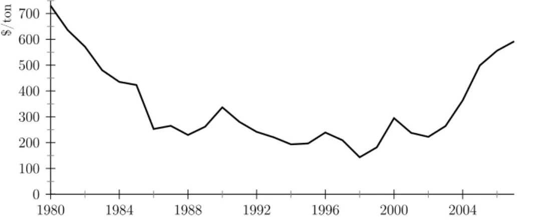
The Jet-Fuel price is expressed in 2000 constant USD per ton. The original series, ex-pressed in current terms, have been obtained from Platts. Figure 5 displays the evolution of Jet-Fuel prices during 1980-2007, which may be used as a proxy of ticket prices. Indeed, according to the literature (Abed Seraj et al., 2001; Battersby and Oczkowski, 2001; Bhadra, 2003; Lai and Lu, 2005; Bhadra and Kee, 2008), the time-series of tickets prices is unobserv-able, or at least hard to investigate empirically.
0 100 200 300 400 500 600 700 1980 1984 1988 1992 1996 2000 2004 $/ to n
Figure 5: Evolution of Jet-Fuel prices during 1980-2007 (expressed in 2000 constant USD per ton). Source: Authors, from Platts.
The time-series of Jet-Fuel prices exhibits a wide variability during the period, going from 143$/ton in 1998 to 730$/ton in 1980. During 1980-1986, the price of Jet-Fuel has been rapidly decreasing as a rebound effect of the second oil crisis. Until 2003, the time-series fluctuated in the range of 150-300$/ton. Due to its strong correlation with the brent crude oil market, Jet-Fuel prices have been rapidly increasing since 2004 (up to 600$/ton), mainly due to dramatic increases in worldwide energy demand.
3.2.2 Econometric specifications
According to the discussion presented in Section 3.1, GDP, Jet-Fuel prices (used as a proxy of ticket prices) and some exogenous shocks should have an influence on air traffic. But the magnitude of the influence of these air traffic determinants seems also to depend on air transport market maturity, which varies widely among the eight geographical regions previously identified.
Following this discussion, the role played by these variables on air traffic is estimated using panel-data modeling. Cross-sectional units of the panel-data sample correspond to the eight zones. Moreover, our panel-data sample is closer to time-series data than cross-sectional data as it contains, in particular, Jet-Fuel prices and the eight geographical regions’ air traffic and GDP time-series. It appears thus suitable to include the lagged dependent variable among the regressors.
Then, we use the following econometric specification using dynamic panel-data models to test for the influence of previously identified air traffic determinants:
lrtki,t = γlrtki,t−1+ x′i,t β+ αi+ ǫi,t (1)
with t={1980, . . . , 2007} the period on which air traffic data have been obtained and i={ Central and North America, Europe, Latin America, Russia and CIS, Africa, the Middle East, Asian countries and Oceania, China} the eight regions considered.
lrtki,t is the log of the i-th region’s air traffic (expressed in RTK) at time t and, as usual, (αi+ ǫi,t) is the composite error term.
x′
i,t is the vector of explanatory variables. x′
i,t = {lgdpi,t, sgrowtht, csgrowtht, sairt, csairt, ljetpricet} where lgdpi,t is the log of the i-th
region’s GDP at time t, sgrowtht is the t-th of a dummy variable for slow-downs in GDP
activity, csgrowtht is the t-th of a dummy variable for counter GDP activity shocks, sairt is the t-th of a dummy variable for shocks specific to the aviation sector, csairt is the t-th of a dummy variable for counter-shocks specific to the aviation sector, and ljetpricetcorresponds – to simplify – to the log of the Jet-Fuel price at time t (see below for a more detailed description regarding the latter variable).
Regarding exogenous shocks, as explained above, two kinds of variables may be computed: (i) slow-down activity shocks, and (ii) aerial-specific shocks. For each category, two kinds of dummy variables have been computed. The first ones (sgrowth and sair) are equal to 1 the year the shock occurs, and 0 otherwise. According to previous literature (Lai and Lu, 2005), air traffic may over-react after these shocks. To test this hypothesis, a second category of dummy variables is used (csgrowth and csair) which are equal to 1 the two years following the shock, and 0 otherwise. Following what was explained in Section 3.1, sgrowth is equal to one for the years 1982, 1991 and 1997 and sair is equal to one for the years 2001 and 2003.
Regarding the Jet-Fuel price variable, ljetprice, two different specifications are investi-gated to uncover the influence of Jet-Fuel price on air traffic demand. As a consequence, the ljetprice variable can be decomposed in two ways. Either ljetprice = (ljetpt), ∀t = {1980, . . . , 2007}, where ljetptis simply the log of the Jet-Fuel price at time t. Or ljetprice =
(ljetpup, ljetpdown), where ljetpup = (ljetpupt−1), ∀t = {1981, . . . , 2007} and ljetpdown = (ljetpdownt−1), ∀t = {1980, . . . , 2007}. The former specification (ljetprice = (ljetpt)) is the most straightforward approach, while the latter specification (ljetprice = (ljetpup, ljetpdown)) takes into account threshold effect of Jet-Fuel price changes (respectively above and below 300 US$).
This leads us to express – and estimate, see below – eq.(1) in two different ways, depending the way Jet-Fuel price is modeling.
The first specification of eq.(1) is:
lrtki,t =γlrtki,t−1+ β1lgdpi,t+ η1ljetpt
+ β2sgrowtht+ β3csgrowtht+ β4sairt+ β5csairt+ αi+ ǫi,t
(2) The second specification of eq.(1) is:
lrtki,t =γlrtki,t−1+ β1lgdpi,t+ η2ljetpupt−1+ η3ljetpdownt
+ β2sgrowtht+ β3csgrowtht+ β4sairt+ β5csairt+ αi+ ǫi,t
(3) Concerning the second specification of the Jet-Fuel price variable (eq.(3)), two kinds of variables have been computed: ljetpup and ljetpdown.
As explained in Section 3.1, above a given threshold (such as 300$/ton), Jet-Fuel prices constitute a significant part of airline companies’ operating costs. Thus, Jet-Fuel prices may have a non-linear effect on air traffic: this variable may impact negatively air traffic, but only above a given price threshold. To test this hypothesis, one variable is computed as a cross-product of a dummy variable – equal to 1 when Jet-Fuel prices’ value is above 300$/ton20and zero otherwise – and of the Jet-Fuel price series. Hence computed, the cross-product variable is equal to the Jet-Fuel price, but only when the latter is above 300$/ton. Therefore, this cross-product variable takes the value of 0 whenever Jet-Fuel prices are below the threshold of 300$/ton.
Moreover, previous literature indicates that this non-linear effect may differ depending on the existence of an upward – or downward Jet-Fuel price trend. Indeed, on an upward (downward) Fuel price trend, airline companies anticipate increasing (decreasing) Jet-Fuel prices. As a consequence, on an upward price trend (above 300$/ton), airline companies purchase Jet-Fuel through forward contracts to limit the anticipated increase in the price of Jet-Fuel. This does not hold necessarily however on a downward price trend.
20
This threshold has been fixed considering the average level of Jet-Fuel prices variation over the whole period (see Figure 5). After experimenting for other thresholds, cross-product variables were only found to be significant as such.
To test for this potential asymmetric non-linear effect, and similarly to the methodology used for the cross-product variable described above, two cross-product variables are computed. First, ljetpup is computed as a cross-product of a dummy variable – equal to 1 when Jet-Fuel prices’ value is above 300$/ton on an upward trend (see Figure 5) and zero otherwise – and of the Jet-Fuel price series. Hence computed, the ljetpup variable is equal to the Jet-Fuel price, but only when the latter is above 300$/ton on an upward trend. Note that this variable is lagged one period to take into account the airline companies’ forward contracting behavior. Second, ljetpdown is computed as a cross-product of a dummy variable – equal to 1 when Jet-Fuel prices’ value is above 300$/ton on an downward trend (see Figure 5) and zero otherwise – and of the Jet-Fuel price series. Hence computed, the ljetpdown variable is equal to the Jet-Fuel price, but only when the latter is above 300$/ton on an downward trend. Contrary to ljetpup, ljetpdown is not lagged because airline companies do not purchase forward contracts in a context of downward Jet-Fuel prices.
Note that the first letter – ‘l’ – figuring at the beginning of ljetpup and ljetpdown indicates that we have taken the log of these two variables when introducing them in eq. (3).
The next section presents the estimates for these two specifications.
3.3
Estimation results and interpretation
The panel-data sample used to estimate eq. (2) and eq. (3) is a long-panel dataset21. More-over, eq.(2) and eq.(3) are characterized by a dynamic structure that specifies the dependent variable for an individual (lrtki,t) to depend in part on its values in previous periods. As a consequence, traditional panel-data estimation approaches (fixed and random effects models) are not appropriate and are not presented here. Indeed, if the lagged dependent variable is included among regressors, the fixed effects needs to be eliminated by first-differencing rather than mean-differencing22.
Our generic econometric specification (Eq. (1)) becomes then:
∆lrtki,t = γ∆lrtki,t−1+ ∆x′i,t β+ ∆ǫi,t (4)
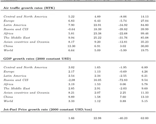
where ǫi,t is now supposed to be serially uncorrelated (this assumption is testable, see below). The descriptive statistics of variables used in eq. (4) are given in Table 223.
21
Long-panel dataset are characterized by a relatively small number of individuals and a relatively long time period (N is small and T → ∞).
22
For a general presentation of dynamic panel-data models, see Cameron and Trivedi (2005).
23
The first-difference of a variable expressed in logarithm may be approximated by its growth rate. This reason explains why Table 2 summarizes descriptive statistics of the growth rates of the explanatory variables of air traffic.
Variable Mean (%) Std. Dev. (%) Min. (%) Max. (%) Air traffic growth rates (RTK)
Central and North America 5.22 4.89 -8.06 14.13
Europe 6.83 6.43 -5.74 27.04
Latin America 7.90 22.91 -34.92 84.80
Russia and CIS -0.64 18.39 -39.82 39.99
Africa 5.81 23.38 -22.68 99.46
The Middle East 9.94 25.22 -31.76 85.08
Asian countries and Oceania 8.17 9.20 -12.81 35.23
China 12.30 6.91 3.02 30,00
World 6.64 5.09 -5.99 19.75
GDP growth rates (2000 constant USD)
Central and North America 3.02 1.65 -1.95 6.89
Europe 2.17 1.13 -0.69 4.26
Latin America 2.54 2.34 -2.55 6.21
Russia and CIS -2,08 16.05 -72.83 9.54
Africa 3.19 1.53 0.06 5.78
The Middle East 2.85 2.91 -2.03 9.60
Asian countries and Oceania 8.21 2.07 2.25 11.33
China 9.89 1.58 7.60 13.10
World 3.33 1.12 0.88 5.15
Jet-Fuel Price growth rate (2000 constant USD/ton)
1.66 22.98 -40.23 62.00
Table 2: Descriptive statistics.
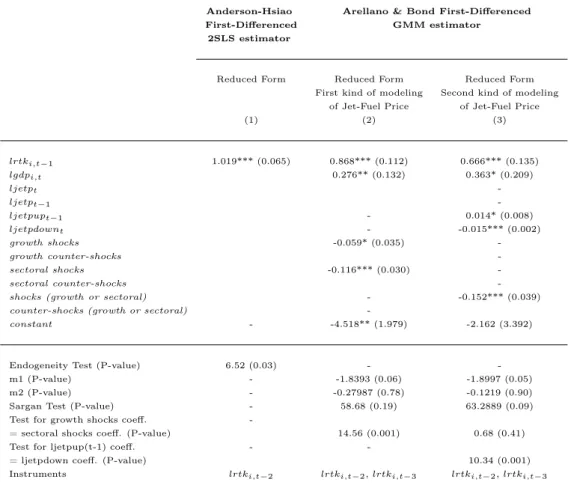
Estimates results are presented in Table 3. Eq. (2) and eq. (3), in first-differences, are estimated using the Anderson–Hsiao (Anderson and Hsiao (1981)) – column (1), Table 3 – and the GMM (Arellano and Bond (1991)) – columns (2) and (3), Table 3 – estimators. Note that these estimates results are only presented in reduced form.
Anderson and Hsiao (1981) proposed IV estimation using lrtki,t−224, which is uncorre-lated with ∆ǫi,t, as an instrument for ∆lrtki,t−1 in eq. (4). The regressors xi,t are used as instruments for themselves as they are strictly exogeneous.
As explained in the previous paragraph, the first column of Table 3 reports the Anderson– Hsiao estimator for eq. (2) and eq. (3) in first-differences. The null hypothesis of the endogeneity test is ‘variables are exogenous’. According to the P − value of this test (P − value= 0.03 < 0.05), one cannot accept this hypothesis when using this estimator.
According to column (1), no explanatory variables, except lrtki,t−1, are statistically sig-nificant: lrtki,t seems thus to follow an AR(1) process when the model is estimating using the Anderson–Hsiao estimator. This result holds whatever the econometric specification of the Jet-Fuel price variable (estimates of either eq. (2) or eq. (3) lead to the same reduced form estimate presented in column (1)). Unsurprisingly, the coefficient of lrtki,t−1 is positive,
24
As indicated in the last line of Table 3. This line indicates, for both estimators, which instruments have been used for ∆lrtki,t−1.
indicating a positive influence of previous air traffic level of the i−th region (lrtki,t−1) on its current air traffic level (lrtki,t).
The last two columns of Table 3 report the estimates results of respectively eq. (2) – column (2), Table 3 – and eq. (3) – column (3), Table 3 – from the (one-step) GMM estimator.
This estimator is also called the Arellano–Bond estimator after Arellano and Bond (1991), who detailed the implementation of the estimator and proposed tests of the assumption that ǫi,t are serially uncorrelated. This estimator may be viewed as an extension to the Anderson– Hsiao estimator. Indeed, the approach of Arellano and Bond (1991) is based on the notion that the estimator proposed by Anderson and Hsiao (1981) does not exploit all the information available in the sample. Compared to the former estimator, the GMM estimator proposes to make a more efficient use of the information in the dataset by using additional lags of the dependent variable as an instrument. By using additional instrumental variables, the GMM estimator proposed by Arellano and Bond (1991) leads to more efficient estimates25.
For a large T (relatively to cross-sectional units), the Arellano–Bond method generates many instruments, leading to a potentially poor performance of asymptotic results26. This argument explains why the number of instruments has been restricted to lrtki,t−2and lrtki,t−3, as shown in the last line of Table 3.
The quality of regressions presented in column (2) and (3) of Table 3 is verified through two specification tests: the serial correlation tests m1 and m2 and a test of overidentifying restrictions (the Sargan Test).
m1 and m2 are tests for respectively first-order and second-order serial correlation, asymp-totically N (0, 1). The null hypothesis of these tests is that Cov(∆ǫi,t,∆ǫi,t−k) = 0 for k = 1, 2 is rejected at a level of 0.05 if P − value < 0.05. If ǫi,t are serially uncorrelated, we expect to reject at order 1 but not at order 2 (or higher orders). According to the P − values of m1 and m2 tests, this is indeed the case for both columns (2) and (3) of Table 3. In each case, the P − value of m1 is equal (or very close) to 0.05. Thus, we reject at order 1 at the level of 0.05. At order 2, ∆ǫi,t and ∆ǫi,t−2 are serially uncorrelated because the P − values are both superior to 0.05 (the P − values of the m2 test are equal to 0.78 and 0.90).
Regarding the second specification test, the Sargan statistic is used to test the validity of the overidentifying restrictions. The null hypothesis of the Sargan Test is ‘overidentifying restrictions are valid’. The P − values of this test are equal to 0.19 for column (2) and 0.09 for column (3). The null hypothesis that the population moment conditions are correct is not
25
This may explain why the Anderson–Hsiao estimator does not pass the endogeneity test.
26
rejected because the P − values > 0.05.
Thus, there is no evidence either from the serial correlation tests or from the Sargan test that reduced forms estimates results presented in columns (2) and (3) of Table 3 are misspecified.
Anderson-Hsiao Arellano & Bond First-Differenced
First-Differenced GMM estimator
2SLS estimator
Reduced Form Reduced Form Reduced Form
First kind of modeling Second kind of modeling
of Jet-Fuel Price of Jet-Fuel Price
(1) (2) (3) lrtki,t−1 1.019*** (0.065) 0.868*** (0.112) 0.666*** (0.135) lgdpi,t 0.276** (0.132) 0.363* (0.209) ljetpt -ljetpt−1 -ljetpupt−1 - 0.014* (0.008) ljetpdownt - -0.015*** (0.002) growth shocks -0.059* (0.035) -growth counter-shocks -sectoral shocks -0.116*** (0.030) -sectoral counter-shocks
-shocks (growth or sectoral) - -0.152*** (0.039)
counter-shocks (growth or sectoral)
-constant - -4.518** (1.979) -2.162 (3.392)
Endogeneity Test (P-value) 6.52 (0.03) -
-m1 (P-value) - -1.8393 (0.06) -1.8997 (0.05)
m2 (P-value) - -0.27987 (0.78) -0.1219 (0.90)
Sargan Test (P-value) - 58.68 (0.19) 63.2889 (0.09)
Test for growth shocks coeff.
-= sectoral shocks coeff. (P-value) 14.56 (0.001) 0.68 (0.41)
Test for ljetpup(t-1) coeff. -
-= ljetpdown coeff. (P-value) 10.34 (0.001)
Instruments lrtki,t−2 lrtki,t−2, lrtki,t−3 lrtki,t−2, lrtki,t−3
Notes:
Sample: 8 geographical regions; 1980-2007.
Dependent variable: lrtki,t, the log of the i-th region’s air traffic (expressed in RTK) at time t. The
variables used in the regressions are built with the logarithms of the data described in Section 3.2 The standard errors (reported into brackets, unless otherwise indicated) are robust standard errors that
permit the underlying error ǫi,tto be heteroskedastic but do not allow for any serial correlation in ǫi,t,
because then the estimator is inconsistent.
***, ** and * indicate 1%, 5% and 10% significance levels, respectively. The null hypothesis of the endogeneity test is ‘variables are exogenous’.
m1 and m2 are tests for first-order and second-order serial correlation, asymptotically N (0, 1). These test the first-differenced residuals.
Sargan test is a test of the overidentifying restrictions for the GMM estimator, asymptotically χ2
.
Table 3: Reduced form estimates results of eq. (2) and eq. (3) in first-differences from the Anderson–Hsiao (column (1)) and the Arellano–Bond (columns (2) and (3)) estimators.
We turn now to the interpretation of these estimates.
from the (one-step) GMM estimator. As in column (1), lrtki,t−1 is statistically significant and its coefficient is positive. This indicates that the current air traffic level of the i−th region (lrtki,t) depends positively on its previous level (lrtki,t−1). Compared to column (1), the lgdpi,t variable is now statistically significant. Its coefficient is positive: the more the GDP of the i−th region is growing, the more its air traffic is growing too. The growth shocks and sectoral shocks variables are both statistically significant and their coefficients are negative. This indicates that air traffic (lrtki,t) effectively overreacts to (i) slow-down activity shocks (the growth shocks variable) and (ii) (negative) aerial-specific shocks (sectoral shocks). The P − value of the test for equality of these two latter variables (see Table 3, third-to-last line, column (2)) is equal to 0.001. Thus, one cannot group these two dummy variables into a single one. Both slow-down activity shocks and aerial-specific shocks have a negative influence on air traffic, but one should not confound these two kinds of shocks. Finally, the price of Jet-Fuel, lagged or not (respectively ljetpt−1 and ljetpt), seems to have no influence on air traffic as the coefficients of these two variables are not statistically significant. Contrary to Dresner (2006) and Graham and Shaw (2008), our estimate result from eq. (2) does not indicate a negative elasticity between ticket prices (proxied by the Jet-Fuel price) and air traffic.
Before concluding to the non-existence of such an elasticity, one may wonder if this latter result is not due to a wrong specification of the influence of the Jet-Fuel price variable on air traffic. Eq. (3) proposes another way to specify the influence of the Jet-Fuel price variable by taking into account price thresholds effects (see Section 3.2 for more details). Column (3) – Table 3 – presents the reduced form estimate of eq. (3) in first-differences from the (one-step) GMM estimator. Coefficients of lrtki,t−1, lgdpi,t and ‘shocks’ variables are not commented, as the same comments as those presented in the previous paragraph apply27. Regarding the new way to specify the influence of Jet-Fuel prices on air traffic, ljetpupt−1 and ljetpdownt are both statistically significant. This result shows that Jet-Fuel prices have a non-linear effect on air traffic28. Moreover the negative coefficient of ljetpdown
t indicates that, above a given price threshold, Jet-Fuel prices have effectively a negative impact on air traffic. The positive sign of ljetpupt−1 seems then counter-intuitive, indicating a positive elasticity between ticket prices (proxied by the Jet-Fuel price) and air traffic. The following reason may explain this seemingly counter-intuitive result. Recall that the ljetpupt−1 variable is the log of the upward
Jet-Fuel price lagged one period. ljetpupt−1 is computed as a cross-product of a dummy
27
Note however the relatively stability of these coefficients between column (2) and column (3), which shows the robustness of our results.
28
This statement is also confirmed by the P − value of the test for equality of the coefficients of ljetpupt−1
and ljetpdownt (see Table 3, second last line, column (3)). This P − value is equal to 0.001, indicating that
variable – equal to 1 when Jet-Fuel prices’ value is above 300$/ton on an upward trend and zero otherwise – and of the Jet-Fuel price series. Thus, according to Figure 5, ljetpupt−1 was equal to the Jet-Fuel price series (lagged one) during the period going from 2003 to 2008. This particular period is characterized by an important increase of energy demand causing a rapidly increase of all energy prices. Thus, the positive sign of ljetpupt−1 may actually just reflect this very particular period.
In the next section, we re-use these econometric results to build different air traffic forecasts scenarii.
4
In-sample prediction and air traffic forecasts
Following the discussion developed in Section 3.3, the reduced form estimate of eq. (3) in first-differences from the (one-step) GMM estimator (Column (3), Table 3) is used to generate air traffic forecasts until 2025. Before presenting these forecasts, in-sample predictions are first presented to assess how our model fits historical data.
4.1
In-sample predictions
After estimating eq. (3) with a dynamic panel-data estimator, one can compute the predicted values of this model. Computing predicted values allows us to generate in-sample predictions: the values of the response variable generated by the fitted model using historical data. Because cross-sectional units of our panel-data sample correspond to the eight geographical regions already presented, the modeling has been realized for each of these eight zones. The response variable of our model is lrtki,t, the log of the i-th region’s air traffic (expressed in RTK) at time t29 (recall eq. (3)). It is thus readily possible to compute our model’ s predicted values of (the log of) air traffic (expressed in RTK) for each of these eight regions during the period 1981-2007. Once each region’s predicted values of air traffic have been computed, it becomes readily possible to re-aggregate these values at the world level. One then obtains predicted values of air traffic (expressed in RTK) at the world level and its 95 % interval predictions.
Figure 6 compares in-sample predicted values of air traffic at the world level (bold line) with ‘true values’ of world air traffic (grey line) during the 1981-2007 period30.
29
With, as already explained, t={1980, . . . , 2007} the period on which air traffic data have been obtained and i={ Central and North America, Europe, Latin America, Russia and CIS, Africa, the Middle East, Asian
countries and Oceania, China} the eight regions considered.
30
0 100 200 300 400 500 600 700 1981 1983 1985 1987 1989 1991 1993 1995 1997 1999 2001 2003 2005 2007 10 9R T K
Grey line: ICAO data; bold line: in-sample predicted values; dashed lines: 95 % Interval Prediction.
Figure 6: In-sample predictions and evolution of world air traffic (expressed in RTK (billions)) between 1981 and 2007.
Figure 6 shows that our model fits historical data quite well at the world level. In-sample predicted values are very close to historical data. The 95 % Interval Predictions (dashed lines) indicate the precision of these estimates. Since the ‘quality’ of our model has been assessed, we may present below air traffic forecasts based on this model.
4.2
Air traffic forecasts until 2025
Air traffic forecasts are obtained by computing out-of-sample predictions. These out-of-sample predictions are generated by applying the estimated regression function of eq. (3) (column (3), Table 3) to observations that were not used to generate the estimates.
It is thus possible to obtain different air traffic forecasts scenarii, depending on the as-sumptions made on the evolution of air traffic drivers previously identified. One needs then to use hypothetical values of the regressors to generate air traffic forecasts. In particular, it has been already underlined that the GDP growth rate is, by far, the most important air traffic determinant. Thus, air traffic forecasts presented below rely on a crucial assumption: the future evolution of the eight geographical regions’ GDP growth rates. The International Monetary Fund (IMF) provides projections of these GDP growth rates until 2014.
Three ‘air traffic forecasts’ scenarii are considered. The main air traffic forecasts scenario - ‘IMF GDP growth rate’ - is based on the GDP growth rates obtained from the IMF World Economic Outlook (WEO) Database. Two other air traffic forecasts scenarii are defined. In the ‘Low GDP growth rates’ air traffic forecasts scenario, the IMF GDP growth rates projections are decreased by 10 %. In the ‘High GDP growth rates’ air traffic forecasts scenario the IMF GDP growth rates projections are increased by 10 %. These two alternative scenarii
are created to measure the sensitivity of air traffic to changes in GDP growth rates.
4.2.1 Analysis at the worldwide level
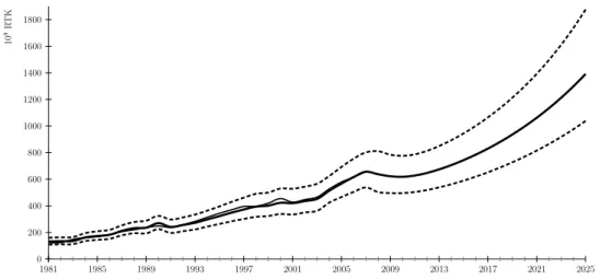
Figure 7 provides a visual representation of our ‘IMF GDP growth rate’ air traffic forecasts scenario – expressed in RTK – at the world level until 2025 (bold line, from 2008 to 2025) and its 95 % Interval Predictions31 (dashed lines, from 2008 to 2025).
0 200 400 600 800 1000 1200 1400 1600 1800 1981 1985 1989 1993 1997 2001 2005 2009 2013 2017 2021 2025 10 9R T K
Grey line: ICAO data; bold line: in-sample predicted values (from 1981 to 2007) and air traffic forecasts (from 2008 to 2025); dashed lines: 95 % Interval Prediction.
Figure 7: World ‘IMF GDP growth rate’ air traffic forecasts (expressed in RTK (billions)) until 2025.
According to Figure 7, our model predicts first a relatively high decrease of air traffic in 2008 and 2009 (-3.47 % between 2007 and 2008) followed by the recovery of its positive evolution from 2010 to 2025. Negative GDP growth rates in 2008 and 2009 explain the predicted decrease of air traffic during this period.
According to our main air traffic forecast scenario, world air traffic (expressed in RTK (109
)) should, overall, increase at a yearly mean growth rate of 4.7%, rising from 637.4 to 1391.8 between 2008 and 2025 (see next section, Table 4). By comparison, the ‘Low GDP growth rates’ and ‘High GDP growth rates’ air traffic forecasts scenarii predict a yearly mean growth rate of world air traffic – expressed in RTK – of 4.2% (Table 5, see the Appendix) and 5.3% (Table 6, see the Appendix), respectively. Thus, a decrease (resp. an increase) by 10%
31
Variances of in-sample predicted values and forecasts are different. As is intuitive, the variances of the forecasts are higher than the variances of the predicted values. This explains the progressively increasing gap between the lower bound and the upper bound of the 95 % Interval Predictions.
of regions’ GDP growth rates previsions yields to a decrease (resp. an increase) of the world air traffic yearly mean growth rate by about 10.6% (resp. 12.8%).
Regarding the evolution of each region’s WLF until 2025, it has been chosen to adopt the following assumptions. Each region’s WLF is assumed to tend to 75%. Thus for each region, we apply the WLF yearly mean growth rate of the period 1996-2006 until the region’s WLF reaches the 75% value. Nevertheless, in order to have a more realistic scenario, assumptions concerning Latin America, Africa and the Middle East are slightly different (see Chèze et al. (2010) for more details).
The conversion of air traffic forecasts expressed in RTK into corresponding air traffic forecasts expressed in ATK yields to estimate how much more filling aircrafts (until 75 % of their capacity) will curb the air traffic increase. According to the ’IMF GDP growth rates’ air traffic scenario, ATK are projected to go from 999.8 ATK (109
) in 2008 to 2041.9 ATK (109 ) in 2025 (Table 4). This increase corresponds to a yearly mean growth rate of 4.3% (Table 4). Using more aircraft capacities will thus curb world air traffic growth rates by 8.5%.
4.2.2 Analysis at the regional level
Regarding regional air traffic forecasts, RTK yearly growth rates range from 3% for Central and North America to 8.2% for China (Table 4). The regions characterized by the highest degree of air transport market maturity (Central and North America and Europe) are also those recording the lowest air traffic growth rates. These results confirm the sensitivity of air traffic drivers to the region’s aviation sector maturity. Note that the two highest yearly mean growth rates are expected in the two Asian regions32, confirming the important growth perspectives of the aviation sector in Asia.
The growth rates for Central and North American and European airlines will be less than the world’s average. According to our forecast, their share in world air traffic will significantly decrease. It will go from 62.61% in 2006 to 51.43% in 2025 (Figure 8). Conversely, the forecast confirms the growing weight of Asian countries and China in world air traffic. Their share will be 36.78% in 2025, while it was 27.12% in 2006 (Figure 8). These trends may be explained by two factors: (i) differences in the GDP growth forecasts (ii) differences in market maturity. Globally, the share of the four others regions should remain stable.
As shown in Table 4, we find similar trends in ATK. The difference in predicted growth rates between RTK and ATK - at the regional and world levels - may be explained by the actual weight load factors and their predicted evolutions. Note that our results are consistent
32
Air traffic (expressed in RTK) mean growth rates of China and Asian countries & Oceania are equal to 8.2% per year and 6.9% per year, respectively.
RTK (109
) Corresponding
Regions (mean growth ATK (109
)
rate per year) (mean growth
rate per year)
2008 2025 2008 2025
Central and North America 246.2 405.9 403.9 627.5
(3.0%) (2.6%)
Europe 163.5 310.0 235.2 413.1
(3.9%) (3.5%)
Latin America 28.5 64.7 47.1 89.3
(5.0%) (3.9%)
Russia and CIS 9.6 21.1 15.4 28.1
(4.9%) (3.8%)
Africa 9.9 30.0 17.3 47.6
(6.7%) (6.2%)
The Middle East 24.1 48.7 39.9 74.3
(4.5%) (4.0%)
Asian countries and Oceania 98.6 296.4 158.2 465.2
(6.9%) (6.8%)
China 56.9 215.0 82.8 296.7
(8.2%) (7.9%)
World 637.4 1391.8 999.8 2041.9
(4.7%) (4.3%)
Notes: Figures into brackets represent yearly mean growth rate of air traffic forecasts between 2008 and 2025. Note that for each zone and at the world level, the yearly mean growth rate of air traffic forecasts expressed in ATK is always inferior to the yearly mean growth rate of air traffic forecasts expressed in RTK.
Table 4: ’IMF GDP growth rate’ air traffic forecasts scenario at the world level (last line) and for each geographical regions (other lines).
2006 2025
Central and Europe
Latin America Russia and CIS
North America Africa
The Middle East
Asian countries and Oceania
China
Figure 8: World repartition by zone of air traffic (expressed in RTK) in 2006 and 2025 according to ’IMF GDP growth rate’ air traffic scenario. Source: Authors, from ICAO data. with previous studies (Airbus, 2009; Boeing, 2009; Mazraati, 2010) confirming that in several regions, air traffic should grow faster than GDP. Moreover, we confirm the growing influence
of China in the aviation sector.
5
Conclusion
This article develops an econometric analysis of the demand for mobility in the aviation sector. The role played by different variables (such as GDP, Jet-Fuel prices, exogenous shocks, market maturity, etc.) on air traffic is estimated by using dynamic panel-data modeling. Then, we use our model to forecast the evolution of air traffic until 2025.
First, we provide detailed descriptive statistics on air traffic, using air traffic data from the ICAO during 1980-2007. We highlight the strongly rising trends in the evolution of worldwide air traffic, along with changes in the composition of air traffic by zone. While the share of Europe and North America in air traffic remained relatively stable over the period, China is becoming a major player in air transportation. Indeed, its share in total air traffic has skyrocketed, going from 4.74% in 1996 to 8.57% in 2006.
According to the previous literature33, the main air traffic drivers are (i) GDP growth rates; (ii) ticket prices; (iii) alternative transport modes; and (iv ) some external shocks such as the September 11 terrorist attacks in 2001. The influence of these drivers depends on air transport market maturity. To take into account the latter criteria, the econometric modeling is carried out by using dynamic panel-data models for eight geographical zones. The influence of the main air traffic determinants is estimated by using the Arellano-Bond estimator. GDP appears to have a positive influence on air traffic, whereas the influence of the Jet-Fuel price - above a given threshold - is negative. Exogenous shocks may also have a (negative) impact on air traffic growth rates. Last but not least, the dynamic panel-data modeling leads us to conclude that the magnitude of the influence of air traffic drivers differs from one region to another.
Once estimated from historical data, the model is used to generate air traffic forecasts. It is thus possible to obtain different air traffic forecasts scenarii, depending on the assumptions made on the evolution of the main air traffic drivers. Various air traffic forecasts scenarii are developed. According to the ’IMF GDP growth rate’ scenario, air traffic is expected to record a rapid growth until 2025. Our results suggest that air traffic (expressed in RTK) will grow at an average yearly growth rate of 4.7 between 2008 and 2025 at the worldwide level (ranging from 3% (Central and North America) to 8.2 % (China), at the regional level).
33
See in particular DfT (2009), ECI (2006), Eyers et al. (2004), Gately (1988), IPCC (1999), Macintosh and Wallace (2009), Mayor and Tol (2010), RCEP (2002), Vedantham and Oppenheimer (1994, 1998), Wickrama et al. (2003).
These results stress the need to take into account the regional heterogeneity when con-sidering the actual and future trends in world air traffic. In particular, the growing weight of the Asian regions in world aviation (driven by high GDP growth rates) constitutes an overwhelming trend.
20 22 24 26 1981 1985 1989 1993 1997 2001 2005 20 22 24 26 1981 1985 1989 1993 1997 2001 2005
Central and North America Europe
20 22 24 26 1981 1985 1989 1993 1997 2001 2005 20 22 24 26 1984 1988 1992 1996 2000 2004
Latin America Russia and CIS
20 22 24 26 1981 1985 1989 1993 1997 2001 2005 20 22 24 26 1981 1985 1989 1993 1997 2001 2005
Africa The Middle East
20 22 24 26 1981 1985 1989 1993 1997 2001 2005 20 22 24 26 1994 1998 2002 2006
Asian countries and Oceania China
Solid line: ICAO data, dashed lines: 95 % Interval Predictions.
RTK (109
) Corresponding
Regions (mean growth ATK (109
)
rate per year) (mean growth
rate per year)
2008 2025 2008 2025
Central and North America 246.2 391.2 403.9 604.8
(2.8%) (2.4%)
Europe 163.5 287.7 235.2 383.5
(3.5%) (3.0%)
Latin America 28.5 62.7 47.1 86.5
(4.8%) (3.7%)
Russia and CIS 9.6 19.1 15.4 25.4
(4.2%) (3.2%)
Africa 9.9 27.6 17.3 43.8
(6.2%) (5.6%)
The Middle East 24.1 42.3 39.9 64.6
(3.7%) (3.2%)
Asian countries and Oceania 98.6 253.8 158.2 398.4
(6.0%) (5.8%)
China 56.9 184.4 82.5 254.5
(7.3%) (6.9%)
World 637.4 1268.9 999.8 1861.5
(4.2%) (3.8%)
Notes: Figures into brackets represent yearly mean growth rate of air traffic forecasts between 2008 and 2025. Note that for each zone and at the world level, the yearly mean growth rate of air traffic forecasts expressed in ATK is always inferior to the yearly mean growth rate of air traffic forecasts expressed in RTK.
Table 5: ’Low GDP growth rate’ air traffic forecasts scenario at the world level (last line) and for each geographical regions (other lines).
RTK (109
) Corresponding
Regions (mean growth ATK (109
)
rate per year) (mean growth
rate per year)
2008 2025 2008 2025
Central and North America 246.2 421.0 403.9 650.9
(3.2%) (2.8%)
Europe 163.5 333.7 235.2 444.8
(4.4%) (3.9%)
Latin America 28.5 66.8 47.1 92.2
(5.2%) (4.1%)
Russia and CIS 9.6 23.4 15.4 31.1
(5.5%) (4.4%)
Africa 9.9 32.7 17.3 51.8
(7.2%) (6.7%)
The Middle East 24.1 56.0 39.9 85.4
(5.4%) (4.9%)
Asian countries and Oceania 98.6 345.7 158.2 542.6
(7.9%) (7.8%)
China 56.9 250.3 82.8 345.4
(9.2%) (8.8%)
World 637.4 1529.5.8 999.8 2244.2
(5.3%) (4.9%)
Notes: Figures into brackets represent yearly mean growth rate of air traffic forecasts between 2008 and 2025. Note that for each zone and at the world level, the yearly mean growth rate of air traffic forecasts expressed in ATK is always inferior to the yearly mean growth rate of air traffic forecasts expressed in RTK.
Table 6: ’High GDP growth rate’ air traffic forecasts scenario at the world level (last line) and for each geographical regions (other lines).
References
Abed Seraj, Y., Ba-Fail, A.O., Jasimuddin, S.M., 2001. An econometric analysis of in-ternational air travel demand in Saudi Arabia. Journal of Air Transport Management 7, 143-148.
Airbus, 2007. Flying by Nature: Global Market Forecast 2007–2026. Report. Airbus, France.
Airbus, 2009. Flying by Nature: Global Market Forecast 2009–2028. Report. Airbus, France.
Alderighi, M., Cento, A., 2004. European airlines conduct after september 11. Journal of Air Transport Management 10(2), 97-107.
Alperovich, G., Machnes, Y., 1994. The role of wealth in the demand for international air travel. Journal of Transport Economics and Policy 28 (2), 163-173.
Anderson, T.W., Hsiao, C., 1981. Estimation of dynamic models with error components. Journal of the American Statistical Association, 589-606.
Arellano, M., Bond, S., 1991. Some Tests of Specification for Panel Data: Monte Carlo Evidence and an Application to Employment Equations. Review of Economic Studies 58, 277-297.
Battersby, B., Oczkowski, E., 2001. An Econometric Analysis of the Demand for Domestic Air Travel in Australia. International Journal of Transport Economics 28(2), 193-204.
Becken, S., 2002. Analysing International Tourist Flows to Estimate Energy Use Associ-ated with Air Travel. Journal of Sustainable Tourism 10(2), 114-131.
Bhadra, D., 2003. Demand for air travel in the United States: bottom-up econometric estimation and implications for forecasts by origin and destination pairs. Journal of Air Transportation 8(2), 19-56.
Bhadra, D., Kee, J., 2008. Structure and dynamics of the core US air travel markets: A basic empirical analysis of domestic passenger demand. Journal of Air Transport Management 14, 27-39.
Boeing, 2009. Current Market Outlook 2009-2028. Report. Boeing, United States. Cameron, A., Trivedi, P., 2005. Microeconometrics: Methods and Applications. Cam-bridge: Cambridge University Press.
Chèze, B., Gastineau, P., Chevallier, J., 2010. Forecasting Air Traffic and Corresponding Jet-Fuel Demand until 2025. Les cahiers de l’économie 77, Série Recherche, IFP School.
Dresner, M., 2006. Leisure versus business passengers: Similarities, differences, and im-plications. Journal of Air Transport Management 12(1), 28-32.
ECI, 2006. Predict and Decide: Aviation, Climate Change and UK Policy. Environmental Change Institute, Oxford.
Eyers, C., Norman, P., Middel, J., Plohr, M., Michot, S., Atkinson, K. and Christou, R., 2004. AERO2k Global Aviation Emissions Inventories for 2002 and 2025. QINETIQ Report to the European Commission, United Kingdom.
Gately, D., 1988. Taking off: the US demand for air travel and jet fuel. The Energy Journal 9(2), 93-108.
Gillen, D. and Lall, A., 2003. International transmission of shocks in the airline industry. Journal of Air Transport Management 9(1), 37-49.
Graham, B., 1999. Airport-specific traffic forecasts: a critical perspective. Journal of Transport Geography 7, 285-289.
Graham, B., Shaw, J., 2008. Low-cost airlines in Europe: Reconciling liberalization and sustainability. Geoforum 39, 1439-1451.
Greene, D.L., 1992. Energy-efficiency improvement of commercial aircraft. Annual Review of Energy and the Environment 17, 537-573.
Greene, D.L., 1996. Transportation and Energy. Eno Transportation Foundation, Inc. Lansdowne, Va, USA, 1996.
Greene, D.L., 2004. Transportation and Energy, Overview. Encyclopedia of Energy 6, 179-188.
Grosche, T., Rothlauf, F., and Heinzl, A., 2007. Gravity models for airline passenger volume estimation. Journal of Air Transport Management 13, 175-183.
Guzhva, V.S., Pagiavlas, N., 2004. US Commercial airline performance after September 11, 2001: decomposing the effect of the terrorist attack from macroeconomic influences. Journal of Air Transport Management 10, 327-332.
Hätty, H. and Hollmeier, S., 2003. Airline strategy in the 2001/2002 crisis-the Lufthansa example. Journal of Air Transport Management 9, 51-55.
ICAO, 2007. Outlook for Air Transport to the Year 2015. International Civil Aviation Organization, AT/134, 1-50.
IEA, 2009a. CO2 Emissions from Fuel Combustion. International Energy Agency, Paris.
IEA, 2009b. Transport, Energy and CO2: Moving Towards Sustainability. International
Energy Agency, Paris.
IEA, 2009c. World Energy Outlook. International Energy Agency, Paris.