Rigid Families for CCS and the π-calculus
Texte intégral
Figure


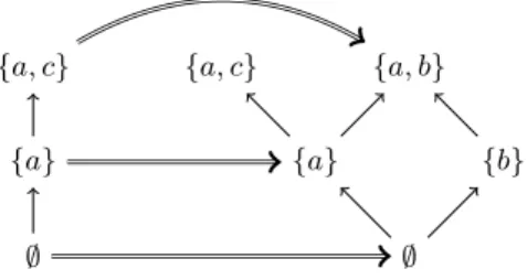
![Fig. 5. The configuration struc- struc-tures of (bhai | chai | a(d))\a in [9]](https://thumb-eu.123doks.com/thumbv2/123doknet/14248776.487894/17.918.515.700.684.833/fig-configuration-struc-struc-tures-bhai-chai-d.webp)

Documents relatifs
This note is devoted to a rigorous derivation of rigid-plasticity as the limit of elasto- plasticity when the elasticity tends to
In this paper, we have presented an interface homogenization for acoustic waves in the time domain; the case of thin periodic roughnesses on a wall and the case of a thin
Irregular locus of the commuting variety of reductive symmetric Lie algebras and rigid pairs..
Our configuration approach builds on our previous work (i.e., Product line Use case Modeling method) and is supported by a tool relying on natural language pro- cessing and
Particularly M1'-F and Mz"-F distances are not equivalent (EXAFS results /5/) and isomorphism substitution is not strict. However, owing to the difficulties, results may
After the internal and external functional analysis is done in ACSP, the user enters the functional parameters in ORASSE Knowledge, because it will be this software, which will
The result of applying our proposed approach on a coffee machine case study shows that it is more efficient to transform a delta model to an annotated one, then model check the
Tolerance allocation implies a decomposition of an allowed variation (product tolerance) in a certain critical product dimension onto dimensions contributing to this variation..
