Billette de Villemeur : Toulouse School of Economics (IDEI & GREMAQ), 21 allée de Brienne, 31000 Toulouse, France
Leroux : Corresponding author. HEC Montréal, CIRANO and CIRPÉE. 3000 chemin de la Côte-Sainte-Catherine, Montréal, QC, Canada H3T 2A7
This paper was written while the first author was visiting the Université de Montréal, whose hospitality is gratefully acknowledged. We wish to thank Jérémy Laurent-Lucchetti and Yves Sprumont for simulating discussions. We are also thankful to seminar assistance at the Ninth International Meeting of the Society of Social Choice and Welfare, the 2008 Canadian Resource and Environment Economics Annual Meeting, as well as the participants to seminars at Université Laval and Ottawa University, to the Montreal Natural Resources and Environmental Economics Workshop and to the Equity in Environmental and Resource Economics Conference (Toulouse, June 09) and to the
Cahier de recherche/Working Paper 10-30
Sharing the Cost of Global Warming
Étienne Billette de Villemeur
Justin Leroux
Abstract:
Due to meteorological factors, the distribution of the environmental damage due to
climate change bears no relationship to that of global emissions. We argue in favor of
offsetting this discrepancy, and propose a
“global insurance scheme” to be financed
according to countries’ responsibility for climate change. Because GHG decay very
slowly, we argue that the actual burden of global warming should be shared on the basis
of cumulated emissions, rather than sharing the expected costs of actual emissions as in
a Pigovian taxation scheme. We characterize new versions of two well-known
cost-sharing schemes by adapting the responsibility theory of Bossert and Fleurbaey (1996)
to a context with externalities.
Keywords: Climate Change, Cost Sharing, Responsibility, Compensation
1
Introduction
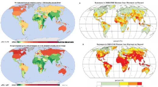
Nowadays, climate change is a notion pervading our collective human psyche, from policy design to everyday conversations, usually under the more casual des-ignation of "global warming". Accompanying our awareness of climatic change is the growing realization that the impacts of global warming are not uniformly distributed across the globe. Yet, by itself, the fact that countries are unequally a¤ected by climate change does not warrant a cry against injustice. Indeed, if the regions most a¤ected by climate change were also the ones contributing to it the most, the observation would be less shocking. However, when comparing maps of recent and cumulated emissions with that of temperature anomalies, one cannot help but notice that they do not coincide (Figure 1). Add to it the fact that the melting of icecaps resulting from climate change will dispropor-tionately impact coastal cities, and it becomes clear that some countries end up generating more harm than they endure, while others must absorb more damage than they cause. In other words, under the near-consensual assumption that the increase in human activity has contributed to climate change, climate change is a prime example of a global externality.
Figure 1. Left, up: per capita GHG emissions by country in 2000; left, down, per capita responsibility in cumulated emissions of GHG. Right, likelihood
that future average summer temperatures exceed the highest temperature observed on record. Up, for the period 2040-2060; down, for 2080-2100. Sources: World Resources Institute, via Wikipedia, for emissions; and Science,
vol. 323 (Jan. 9th, 2009) for temperatures.
Yet, because the discrepancy between the distribution of GHG emissions in the atmosphere, and their resulting impacts, is due to "natural" phenomena (e.g., winds, currents, the melting of icecaps, etc.), and because it is impossible to trace back to its origin the damage borne by any given region, we argue that the distribution of damages lies beyond the responsibility of any country. Nonetheless, provided the aggregate environmental impact of climate change as well as emissions patterns of each country are observable, one can hope to solve this global cost-sharing problem of sorts.
We argue in favor of a global insurance scheme that washes out di¤erences in the distributions of damages, for which countries are not responsible. Similarly, the …nancing of this scheme should holds countries responsible for the (global)
damage for which they are indeed responsible.
A standard approach to implementing the …rst-best level of pollution is through Pigou taxes (or equivalent schemes), which succeed by making polluters internalize the social marginal cost of their externality (pigou, 1932; Baumol, 1972; Nordhaus, 1992). While the "polluter pays" principle behind this ap-proach is very appealing, Pigou taxation can only perform satisfactorily when the social marginal cost can be reasonably well approximated. However, given that the lifetime of GHG emissions may last more than hundreds or even thou-sands of years (see Archer, 2005, and Archer and Brovkin, 2008), Pigou taxation is based on expected costs of uncertain events far o¤ in the future, which are very di¢ cult to estimate in practice (Stern 2008). In addition, Pigou taxa-tion is silent on the questaxa-tion of discounting these future costs over hundreds of years and on the normative question of intergenerational equity. Lastly, even if the …rst-best level of emissions is reached, some climate change will occur (as a result of past and current emissions), because some pollution is e¢ cient. Pigou taxation does not explicitly handle the normative question of horizontal (or intra-generational) equity raised by the imbalance between the distribution of emissions and the distribution of damages.
We propose an alternative approach to Pigou taxation which overcomes the shortcomings identi…ed above while remaining entirely compatible with the Pigovian outcome (i.e., a …rst-best pollution level). The key feature of our ap-proach is that it does not rely on estimates of future costs, but rebalances the distribution of current (known) damages each period, thus also circumventing the issue of discounting. Within each period, we treat the issue as a traditional cost-sharing problem, where damages depend on countries’ past and current emissions. We address the issue of global equity by expliciting the responsibility of countries to the global damage according to their past and current emissions
as well as other characteristics (GDP, geographical location, population, etc.). We are fully aware that the debate on countries’responsibilities for past emis-sions is still raging, and it is a debate which is beyond the scope of this work. Nonetheless, our approach is ‡exible enough to accomodate the most prominent competing ideologies, precisely because we let the planner decide explicitly the characteristics for which countries are to be held responsible.
More precisely, the responsibility/compensation approach we adopt is re-lated to that in Bossert & Fleurbaey (1996) in that the planner’s …rst decision is to identify for which characteristics countries should be held responsible and for which characteristics they should be held "non responsible"— and thus com-pensated. For instance, in our context, the planner may deem that current populations are responsible for their current GHG emissions and must there-fore pay for all the resulting damages, but that they are not responsible for their geographical location and corresponding climate, and that their cost share should not depend on their geographical location, all else equal (emissions, in particular). Yet, a tension already arises from this seemingly innocent deci-sion. For example, according to the planner, a country which experiences cold winters, like Canada, should be held responsible for its emissions but at the same time should be compensated for the fact that its emissions are high due to heating needs. In fact, it has been established (Bossert, 1995) that holding economic agents fully responsible for some characteristics was incompatible with full compensation along the other characteristics unless the cost function is sep-arable along the responsibility/compensation dimensions. Because one cannot reasonably assume such separability, the two taxation schemes that will stand out from our analysis (the Egalitarian Equivalent and the Conditionally Equiv-alent mechanisms) result from compromises between full compensation and full responsibility.
From a policy standpoint, our …ndings show that environmental taxation à la Pigou, which is often considered the epitome of responsibilization, pop-ularized by its implementation of the …rst-best pollution levels, is compatible with a modicum of compensation for di¤erences in irrelevant characteristics. In particular, the Conditionally Equivalent solution can be viewed as a Pigou tax followed by redistributive transfers. To the best of our knowledge, it pro-vides the …rst axiomatic speci…cation of how to allocate the Pigou tax revenues, both to wash out the damages su¤ered by each country, and for cross-country compensation.
1.1
A reverse approach to taxation
The leveling of environmental damage presented above requires possibly large funds, equal to the sum of all climate-change-related damage across the globe. Indeed, if we denote by ditthe environmental damage su¤ered by country i due to climate change over a given period, t, the total amount of funds necessary to cancel out the damage for all countries in that period adds up to Dt P
i;tdit.1 Obviously, given the global nature of the issue, the …nancing of the levelling compensation must be collectively borne by the very same countries which are receiving these compensations. Hence, the leveling compensation is, in essence, a redistribution mechanism designed to counter the arbitrary nature of the distribution of climate-change damage across the globe.
Two arguments are in order. First, given that we consider climate change to be closely related to GHG emissions, we argue that the damage-o¤setting scheme should be …nanced in relation to the countries’emission levels, via a tax on emissions of sorts.2 Ideally, this tax should be set so as to achieve e¢ cient 1The dynamic nature of the problem and the relation between damage and carbon emissions
will be made explicit below, as needed in the argumentation.
emission levels. However, we take the view that emissions are like environ-mental debt issued by polluters at all times s < t, a portion of which will be collected over time in the form of the environmental damage Dt. Therefore, unlike the common Pigovian view that the emissions tax should be set equal to the discounted expected future social marginal damage (Nordhaus, 1992), the mechanism we propose repays the "debt", Dt, of observed environmental dam-age each period. Thus, our approach avoids the problematic issue of accurately evaluating expected future costs of uncertain future events, which proves ex-tremely di¢ cult in practice (see, e.g., Stern’s AEA presidential address 2008). This task is all the more di¢ cult as carbon emissions may persist in the at-mosphere for up to thousands of years, thus making unrealistic the estimation of future damage so far in the future. Instead, by basing the emissions tax on current observed environmental damage, our mechanism circumvents this di¢ cult estimation issue entirely3.
An additional bene…t of our "reverse" approach compared to the forward-looking one is that it circumvents another very problematic issue related to the large lifetime of CO2emissions: intergenerational discounting. Indeed, discount-ing beyond several decades already poses the delicate question of how to consider future costs or bene…ts. In other words, it is not just the discount rate itself which is contentious, but the very nature of the discounting (e.g., exponential versus hyperbolic, see Henderson and Bateman, 1995). With the timespans in-volved by CO2emissions covering possibly hundreds or even thousands of years, it seems foolish to envision being able to reach any non-controversial present val-ues of environmental damage. By contrast, our "reverse" approach bypasses the issue entirely due to the fact that period-per-period optimizing countries will
unrelated to human activity. In that case, the rest of our analysis can be interpreted as tackling the issue of the arbitrariness of climate change— which is considered to be happening, regardless of the causes.
3Evaluating current damages remains a di¢ cult task, but a considerably less daunting one
behave as if they had anticipated expected future damage. Indeed, we show by a simple dynamic programming argument in a companion paper (Billette de Vllemeur and Leroux, 2010) that the usual, forward-looking Pigovian tax, un-der rational expectations, coïncides with our "reverse" scheme. The intuition is that each country would correctly anticipate the impact of its current emissions on future damages and respond according to its own discount rate.
1.2
Compensation and responsibility
We now address the question of who will pay how much. Given our responsibility-based approach to fairness, this …nal discussion amounts to sorting out the responsibility of each country in the matter. We adopt the following general principle: "Countries should pay for damage caused for which they are respon-sible and be compensated for damage su¤ered for which they are not". Hence, our approach allows one to make recommendations based on the planner’s as-signment of responsibilities (which is beyond the scope of this work). More precisely, the resulting cost shares will be tailored to re‡ect this assignment of responsibilities, whether it considers that countries are fully responsible for all historical emissions (what we call the Historical Responsibility view) or whether one deems climate change to be independent of CO2 emissions (what we call the External Shock view).
Our approach is related to that of Bossert (1995) and Fleurbaey and Bossert (1996) in that we separate country charateristics into two categories: that of "relevant" characteristics for which countries are deemed responsible and which are related to climate change (i.e., possibly past and present emissions), and "irrelevant" characteristics for which countries should not be held responsible or which are unrelated to climate change (i.e., aspects of geographical location like latitude and coastality; and possibly emissions, depending on the point of
view). Then, we formulate axioms which any taxation rule must verify to be compatible with the desired view of responsibility adopted by the planner.
Ideally, one would want to hold countries fully responsible for di¤erences in their relevant characteristics while being fully compensated for di¤erences in their irrelevant characteristics. Unfortunately, a strong tension exists between these considerations of responsibility and compensation, making them typically incompatible in their strong versions except for unreasonably simplistic case of a linear damage function. Therefore, when deciding on what sharing rule to implement, the planner faces a trade-o¤ between relaxing the extent to which countries are held responsible for their relevant emissions and the extent to which they can be compensated for di¤erences in irrelevant characteristics. The type of cost-sharing mechanisms that emerge from our analysis consists in holding countries responsible— or compensating them— for di¤erences in characteristics, not among themselves per se, but relative to a reference level. Thus, while still taking di¤erences in characteristics into account, cost allocation becomes mathematically feasible, at the expense of being able to charge strictly according to marginal costs. Hence, the possible solutions we o¤er will di¤er in how strongly they depart from marginal-cost pricing.
More speci…cally, one of the two solutions we propose, the Egalitarian Equiv-alent mechanism, splits the consequences of deviations from a reference vector of irrelevant characteristics while sharing equally the residual impact of global warming, once each country has paid for its incremental contribution4. In other words, the Egalitarian Equivalent mechanism prices emissions at incremental cost while balancing the budget via lump-sum transfers based on countries’ir-relevant characteristics. In the responsibility-compensation spectrum, one could argue that the Egalitarian Equivalent mechanism insists on compensation at the 4The incremental cost is the additional cost imposed by the presence of an additional agent,
as opposed to an additional unit of emissions (as is the case for marginal cost). Clearly, the smaller the emissions of a country, the closer the incremental cost is to the marginal cost.
expense of responsibility.
Symmetrically, the second solution we propose, the Conditionally Equivalent mechanism guarantees each agent the average payo¤ of a hypothetical situation in which all countries have the characteristics they are responsible for equal to a reference level. Each country bears the consequences of any deviation from this reference level. As such, the Conditionally Equivalent mechanism insists on countries’responsibility at the expense of compensation considerations. Because countries are (marginally) taxed according to marginal damage, it is akin to Pigou taxation, thus implementing the …rst-best level of emissions.
Our compensation-responsibility approach builds upon that developed in Bossert (1995) and Bossert and Fleurbaey (1996) after adapting it to a context of externalities. Indeed, their setting focuses on wealth redistribution in the ab-sence of externalities, which would be tantamount to assuming a damage func-tion which is separable in the countries’ emissions levels. Such an assumpfunc-tion would be ill-adapted in our context. By contrast, our setup introduces inter-dependence between the countries’characteristics (emission levels) through the damage function. As a result, the analysis allows for applications in more gen-eral settings where externalities are present. Moreover, our results con…rm and extend the appeal of the Egalitarian Equivalent and the Conditionally Equiva-lent solutions to the more general context of externalities.
2
The model
Let S = f1; :::; mg N be the set of countries5. We denote by nithe population of country i and by n = (n1; :::; nm) 2 Nm the population pro…le. We write N =Pmi=1ni. We denote by xi = (xpi; xci) 2 R2 country i’s vector of past and 5We use the word "countries" for simplicity, but our analysis readily applies to regions,
current6 per capita emissions, by xp = (xp1; ::xnp) and xc = (xc1; ::xcn) the past and current per capita GHG emissions pro…les, respectively.7
Each country’s per capita private current bene…ts are associated to its own emissions levels via a mapping bi : R2+ ! R, (x
p
i; xci) 7! bi(x p
i; xci),8 which is continuous and non-decreasing in each argument. We assume bene…ts to be fully transferable across countries. Let b = (b1; ::; bm) be the pro…le of per capita bene…t functions, one per country. We interpret the di¤erences in the bene…t functions across countries to be essentially geographic in nature (latitude, altitude, coastality, etc.).9
In contrast with private bene…ts, which are solely dependent upon a coun-try’s own emissions, per capita country environmental damage will depend on total emissions. More precisely, let X = Pi=1;:::;mnixi be the total level of emissions, where xi = xpi + xci designates country i’s cumulated emissions10. Whenever convenient, we write X i=Pj6=injxjFormally, we denote by di(X) the current per capita damage incurred by country i. We do not make any as-sumption on the functions di(X) other than continuity. In particular, it may be the case that some countries actually bene…t from global warming for some values of X. That is to say we do not exclude the possibility that di(X) < 0 6From a practical standpoint, current emissions can be interpreted as emissions in the very
recent past, say, between 5 and 8 years. This time frame could coincide with the reevaluation periods of the major international protocols (Kyoto, Copenhagen, etc.).
7To lighten notation, we do not index variables by their time subscript. It will be implicit
throughout that all the analysis takes place at time t, and that xc= xc
twhile xp=
P
s<txcs.
More generally, any value decribed as "current" will refer to a value at time t.
8While b
iis not necessarily independent of the country’s population, ni, we do not explicitly
consider variations in ni. Moreover, we make no hypothesis on how bishould vary with ni. 9We formulate the model on a per-capita basis in order to account for the relative sizes
of the various countries. Given the large heterogeneity in country size across the globe, per-country considerations would bias the analysis.
1 0For simplicity, we assume n
ito be constant over time. While this assumption is unrealistic,
its consequence is mainly one of accounting. Our goal is to focus on the role of relevant and irrelevant characteristics. It will become clear that we view population as a "neutral" variable, i.e., belonging to neither category.
for some countries: Nonethless, we assume total damage, D (X) = m X i=1 nidi(X) ;
to be positive and non-decreasing in X: We denote by d = (d1; :::dm) the pro…le of per capita damage functions. Finally, we call (n; b; d; xp; xc) a global warming problem and denote by P the class of such problems.
Our goal is to design a transfer schedule to correct the arguably uneven dis-tribution of damage due to global warming while providing incentives for coun-tries to reduce their emissions, possibly up to inducing full e¢ ciency. Formally, this amounts to compensating every country for the per capita damage it incurs, di(X), while setting up vectors of per capita transfer payments, ti(n; b; d; xp; xc), to …nance the total amount compensated: Piniti(n; b; d; xp; xc) = D(X). The per capita payo¤ of country i is then bi(xpi; xci) ti(n; b; d; xp; xc). We are in-terested in transfer functions, t : P ! Rn which (potentially) hold countries responsible for their past and current emissions levels, xpi and xc
i, while fully washing out the damage su¤ered, di.
Throughout the paper, we consider that countries are not responsible for their damage function, di, nor their bene…t function bi. Moreover, we consider a country’s population, ni, to be a "neutral" characteristic in the sense that it does not warrant compensation (it is not an irrelevant characteristic) nor reward (it is not a relevant characteristic). We contrast several views of responsibility regarding emissions. First, since the cost of global warming depends upon to-tal emissions, one may argue that countries should be held responsible for all of their emissions, both past and current: We shall call this view Historical Responsibility (hereafter HR). Second, one may argue instead that countries should not be held responsible for emissions that go back to a time when the im-pact of GHG emissions on climate change had not been suspected. According to
this view, past emissions are irrelevant and countries should be held responsible only for current emissions levels xc= (xc
1; :::; xcm). We refer to it as no Historical Responsibility (hereafter nHR). Third, past emissions may be considered a natural benchmark to measuring countries’“needs”. According to this so-called Grand-Fathering view (hereafter GF), countries are held responsible for vari-ations between current and past emissions levels xGF = (xGF
1 ; :::; xGFm ); where xGF
i = xci x p
i, for some parameter possibly re‡ecting technical progress. Finally, some still argue that no causal link between human emissions and cli-mate change can be ascertained. According to this fourth viewpoint, which we shall call the External Shock view ( henceforth, ES), countries’emissions levels are irrelevant in redistributing the costs associated with climate change. Note that the ES view is not at odds with the desire to redistribute the impacts of climate change; it simply assumes that damages are not caused by emissions.11 Prior to further investigating the concepts of responsibility and compensa-tion in a global warming context, we impose two minimal fairness requirement. Anonymity requires countries with identical characteristics to be treated equally, while Solidarity asks that no country bene…ts from seeing the damage of other countries suddenly increase, all else equal.12
Axiom 1 (Anonymity) For any P = (n; b; d; xp; xc) 2 P, and any i; j 2 S,
(bi; xpi; x c
i) = (bj; xpj; x c
j) =) ti(P ) = tj(P )
Axiom 2 (Solidarity) For any P = (n; b; d; xp; xc) and P0 = (n; b; d0; xp; xc) 1 1For readibility, the remainder of the paper formulates the global warming problem
accord-ing to the HR view. The correspondaccord-ing results obtained under the other views of responsibility and can be found in the Appendix.
1 2See, e.g., Thomson (2003) for a comprehensive survey of the use of these standard axioms
such that d0j dj for all j 2 S, bi(xpi; x c i) ti(P0) bi(xpi; x c i) ti(P ); for all i 2 S:
3
Responsibility and compensation
3.1
Penalizing (or rewarding) for di¤erences in relevant
characteristics
If countries are considered to be responsible for— at least some of— their emis-sions, di¤erences in these emissions should a¤ect their …nal payo¤s. In fact, a strong interpretation of responsibility consists in holding countries fully respon-sible for the damage they contribute to causing via "relevant" emissions, for which they are considered responsible, irrespective of other, "irrelevant" emis-sions, if any. A …rst approach to responsibility consists in arguing that whatever the distribution of irrelevant characteristics, changes in one country’s relevant characteristics, should a¤ect only this country. This yields:
Axiom 3 (FMR) Full Marginal Responsibility:
Consider a change from P to ^P where some country i’s emissions change from (xpi; xci) to (^xpi; ^xci), all else equal13, then:
ti P^ ti(P ) =
D X^ D (X) ni
;
and tj P^ = tj(P ) for all j 6= i:
1 3We opted for an informal statement for the sake of readability. Formally, the statement
should read: "For any i 2 S, and any P , ^P 2 P such that (^n; ^b; ^d) = (n; b; d)and (^xpj; ^xc
j) =
(xpj; xc
Full Marginal Responsibility is a very demanding axiom as it requires each country to pay the full marginal cost of its own emissions. In fact, it follows from a familiar argument in the cost-sharing literature (e.g., Leroux, 2004) that unless D is linear, no budget-balanced transfer function satis…es FMR:
Proposition 1 No cost-sharing mechanism satis…es FMR unless the damage function, D, is linear in total emissions, X:
Proof. See Appendix A.3.1
This negative result is due to the fact that the notion of marginal damage becomes blurry for non-linear damage functions. This leads us to considering a less demanding axiom, which insists on assigning marginal responsibilities when damage is linear:
Axiom 4 (LMR) Linear Marginal Responsibility:
Suppose individual damage functions are linear. Consider a change from P to ^
P where some country’s emissions change from (xpi; xc i) to (^x
p
i; ^xci), for some i, all else equal, then:
ti P^ ti(P ) =
D X^ D (X) ni
;
and tj P^ = tj(P ) for all j 6= i
Solidarity and LMR together imply that one should charge countries a per-unit cost equal to the average (and marginal) global damage.
Proposition 2 LMR and Solidarity imply Average Damage Pricing:
ti(P ) = xi D (X)
Proof. See Appendix A.2.1.
Hence, it would seem that the rather weak axiom of LMR points to a strong characterization of average damage pricing. While formally correct, we argue that this result relies heavily on a reference level (zero emissions) which we deem inappropriate in our context: granting such a special role to the unattainable (and undesirable) outcome of zero emissions is ill-suited to handling an e¢ cient, or merely a realistic emissions level. Instead, we allow for the planner to de-cide on the appropriate reference emissions level ~X. In practice, this reference level, ~X, can be thought of as a target emissions level. In that case, the ratio D(X) D( ~X)
X X~ approximates the notion of marginal damage around the reference level ~X. The corresponding axiom, Full Reference Responsibility asks that coun-tries be held responsible for departures from the reference level on a per capita basis:
Axiom 5 (FRR) Full Reference Responsibility: Let (~xp; ~xc) 2 R2
+ be a reference vector of per capita emissions and de…ne total reference emissions accordingly: eX = Pj=1;:::;mnj x, with ~~ x = ~xp+ ~xc. For any P = (n; b; d; xp; xc) 2 P, and any ~P = (n; b; d; ~xp 1m; ~xc 1m) 2 P, where 1m stands for the m-unit vector,
ti(P ) ti P~ = (xi x)~ 2 4D (X) D ~ X X X~ 3 5 ; for all i 2 S:
Remark 1 Clearly, if the damage function, D, is linear, FMR and FRR coin-cide.
A complementary interpretation of responsibility is that each country must pay the incremental damage it imposes onto the rest of society:14
ti(P ) ti(P jxi=(0;0)) =
D (X) D (X i)
ni :
Holding countries responsible only for their relevant characteristics implies that the transfer ti(P jxi=(0;0)) should not depend on characteristics for which
coun-tries are not deemed responsible:
Axiom 6 (ECEIC) Equal Contribution for Equal Irrelevant Charac-teristics15 [bi= bj] =) ti(P ) D (X) D (X i) ni = tj(P ) D (X) D (X j) nj :
A weaker version only requires an equal contribution when all countries’ irrelevant characteristics are identical to a reference.
Axiom 7 (ECRIC) Equal Contribution for Reference Irrelevant Char-acteristics.
Consider a reference bene…t function, ~b, then: If bi= ~b for all i 2 S, then:
ti(P ) D (X) D (X i) ni = tj(P ) D (X) D (X j) nj for all i; j 2 S.
Remark 2 Clearly, F M R is a more demanding axiom than F RR, and ECEIC 1 4The shorthand notation P j
xi=(0;0)designates a global warming problem identical to P in
every way except for country i’s emissions, which are zero. Recall that we are adopting the HRview of responsibility. For instance, under the nHR view, the analog would be P jxc
i=0.
1 5This axiom, and others considered here, result from adapting axioms found in Bossert
is more demanding than ECRIC. However, no such relationship exists between F RR and ECEIC.16
3.2
Compensating for di¤erences in irrelevant
character-istics
A …rst approach to dealing with the issue of compensation consists in arguing that di¤erences in irrelevant characteristics should not drive their welfare. In other words, only di¤erences in relevant characteristics should matter.
The above argument can be interpreted to mean that all should equally su¤er— or bene…t— as a result of a change in one country’s irrelevant character-istic:
Axiom 8 (GSIC) Group Solidarity towards Irrelevant Characteristics. Consider a change from bi to ^bi, for some i, all else equal. Denote P = (n; b; d; xp; xc) and ^P = (n; ^b; d; xp; xc), then:
tj(P ) tj P^ =h^bi(xpi; xci) ti P^ i
[bi(xpi; xci) ti(P )]
for all j 6= i.
Remark 3 Under GSIC, budget balance implies
ti(P ) ti P^ = (1 ni N)(bi(x p i; xci) ^bi(x p i; xci)); and tj(P ) tj P^ = ni N(bi(x p i; x c i) ^bi(xpi; x c i)) for all j 6= i.
Another interpretation of compensation consists in requiring that citizens 1 6In the absence of externalities, FMR coincides FRR and implies ECEIC (Bossert and
of two countries with identical relevant characteristics should end up with the same payo¤:
Axiom 9 (EPER) Equal Payo¤ for Equal Responsibility. For all i; j 2 S, [xi= xj] =)
bi(xpi; xci) ti(P ) = bj(xpj; xcj) tj(P ) :
A considerably weaker version of the above axiom requires …nal payo¤ equal-ity only in when the relevant characteristics of all countries are equal to a given reference level.
Axiom 10 (EPRR) Equal Payo¤ for Reference Responsibility. Let (~xp; ~xc) 2 R2
+ be a reference vector of per capita emissions. If (x p i; xci) = (~xp; ~xc) for all i 2 S, then:
bi(xpi; xci) ti(P ) = bj(xpj; xcj) tj(P ) ;
for all i; j 2 S:
Remark 4 Clearly, EPER is more demanding than EPRR. However, no such relationship between GSIC and the other two axioms.17
3.3
Tension between compensation and responsibility
As it turns out, it is generally impossible to compensate countries for di¤erences in irrelevant characteristics while penalizing or rewarding them for di¤erences in relevant characteristics, at least in the strong interpretation of these concepts. In fact, even when D (X) is linear, FMR (or FRR) and GSIC are incompatible 1 7If population had been considered an "irrelevant" characteristic, then GSIC would be
unless the bene…t function is additively separable in countries’ relevant and irrelevant characteristics.
Proposition 3 Suppose D is linear. GSIC and FMR are incompatible unless all bene…t functions are identical up to a constant; i.e, unless there exists a vector 2 Rn and a function h : R2
+! R such that
bi(xpi; xci) = i+ h(xpi; xci)
for all (xpi; xci) 2 R2+:
Proof. In Appendix A.3.2.
Consequently, the only way to reconcile the concepts of compensation and responsibility is to weaken at least one of the two axioms. We discuss these weakenings in turn and characterize the corresponding mechanisms in the next section.
4
The Egalitarian Equivalent and the
Condition-ally Equivalent mechanisms
4.1
The Egalitarian Equivalent mechanism
The Egalitarian Equivalent mechanism splits the consequences of deviations from a reference vector of irrelevant characteristics while sharing equally the residual impact of global warming, after each country has paid for its incremental contribution:
De…nition 1 Egalitarian Equivalent transfer:
for any i 2 S, tHR EEi (P ) = bi(xpi; x c i) ~b (x p i; x c i) + 1 ni[D (X) D (X i)] (1) m X j=1 nj N h bj xpj; xcj ~b xpj; xcj i 1 N 0 @ m X j=1 [D (X) D (X j)] D(X) 1 A :
The Egalitarian Equivalent mechanism is characterized by the combination of GSIC and ECRIC.
Theorem 1 A transfer schedule, t, satis…es GSIC and ECRIC if and only if
t = tHR EE:
Proof. See the Appendix A.2.2.
Remark 5 The above characterization is tight: the strengthening of ECRIC into ECEIC yields an impossibility. Indeed, the reader can check that the EE solution does not satisfy ECEIC.
4.2
The Conditionally Equivalent mechanism
The Conditionally Equivalent mechanism guarantees each agent the average payo¤ of a hypothetical situation in which all countries’relevant characteristics are equal to a reference level. Each country bears the consequences of any deviation from this reference level. Formally,
De…nition 2 Conditionally Equivalent (CE) transfer:
Let P 2 P and consider a reference vector of relevant characteristics (~xp; ~xc) 2 R2+.
For any i 2 S, tHR CEi (P ) = bi(~xp; ~xc) + (xi x)~ 0 @D (X) D ~ X X X~ 1 A (2) 1 N 0 @ m X j=1 njbj(~xp; ~xc) D( ~X) 1 A ; where ~X = Pj2Nnj x:~
The CE mechanism is characterized by FRR and EPRR.
Theorem 2 A transfer schedule, t, satis…es FRR and EPRR if and only if
t = tHR CE:
Proof. See Appendix A.2.3.
Remark 6 The above characterization is tight: the strengthening of EPRR into EPER yields an impossibility. Indeed, the reader can check that the CE solution does not satisfy EPER.
5
Conclusion
The following table summarizes the relationship between the axioms considered thus far.
Table 1
Axioms GSIC EPER EPRR
FMR x x x
FRR x x tCE
ECEIC x x x
ECRIC tEE x x
As in the theory on responsibility and compensation formalized by Bossert (1995) and Bossert and Fleurbaey (1996), the Egalitarian Equivalent and the Conditional Equivalent solutions play a key role. These …ndings con…rm the importance of these solutions, even in settings where externalities are present. However, unlike in Bossert and Fleurbaey (1996), the (equivalent of) axioms ECEIC and ECRIC are generally incompatible with both EPER and EPRR.18 This is due to the fact that we consider population to be a "neutral" charac-teristic. Yet, population is a crucially important characteristic of the problem at hand due to the fact that our approach to responsibility is at the per capita level while data on the characteristics considered (emissions and bene…ts in par-ticular) are likely to only be available at the aggregate level. This dichotomy inevitably places special emphasis on the population characteristic. Yet, while we do not deem individuals responsible for the population of the country they belong to (i.e., population is not a relevant characteristic), we do not believe the taxation scheme should compensate or penalize them for it (i.e., population is not an irrelevant characteristic either). These practical considerations illustrate the necessity of formally introducing a third type of characteristics— "neutral" characteristics— in the axiomatic analysis to responsibility and compensation. To the best of our knowledge, no general theory has been established that con-siders neutral characteristics.
References
[1] Archer, D. (2005) "Fate of fossil-fuel CO2in geologic time", J Geophysical Res, 110 C09S05.
[2] Archer, D. and V. Brovkin (2008) "The millenial atmospheric lifetime of anthropogenic CO2", Climatic Change, 90 283-297.
[3] Baumol, W.J. (1972) "On Taxation and the Control of Externalities", Amer. Econ. Rev., 62 307-322.
[4] Billette de Villemeur, E. and J. Leroux (2010) "Looking forward versus looking backward in environmental taxation", mimeo.
[5] Bossert, W. (1995) "Redistribution mechanisms based on individual char-acteristics", Math. Soc. Sci., 29 1-17.
[6] Bossert, W. and M. Fleurbaey (1996) "Redistribution and Compensation", Soc. Choice Welfare, 13 343-355.
[7] Henderson, N. and Bateman, I. (1995), “Empirical and Public Choice Ev-idence for Hyperbolic Social Discount Rates and the Implications for In-tergenerational Discounting”, Environmental and Resource Economics, 5, 413-423.
[8] Leroux, J. (2004), “Strategyproofness and e¢ ciency are incompatible in production economies”, Economics Letters, 85, 335-340.
[9] Nordhaus, W.D. (1992) "The ecology of markets", Proc. Natl Acad. Sci., 89 843-850.
[10] Pigou, A.C., The Economics of Welfare, 4th ed., London, 1932.
[11] Stern, N. (2008) "The Economics of Climate Change", Amer. Econ. Rev.: Papers and Proceedings, 98 1-37.
[12] Thomson, W. (2003) "Axiomatic and game-theoretic analysis of bank-ruptcy and taxation problems: a survey," Math. Soc. Sci.,.45 249-297.
A
Appendix
A.1
Other views on responsibility
As we mention in the body of the paper, several views of responsibility can be considered to tackle the global warming problem. We describe below how the analysis would be a¤ected by considering the nHR, the GF or the ES view.
A.1.1 Penalizing (or rewarding) for di¤erences in relevant charac-teristics
Axiom 3 (FMR) Full Marginal Responsibility:
nHR-FMR Consider a change from P to ^P where some country’s emissions change from (xpi; xci) to (xpi; ^xci), for some i, all else equal, then:
ti P^ ti(P ) =
D X^ D (X) ni
;
and tj P^ = tj(P ) for all j 6= i: GF-FMR Let xGF
i = xci x p
i: Consider a change from P to ^P where some country’s emissions change from (xpi; xGF
i ) to (x p
i; ^xGFi ), for some i, all else equal, then:
ti P^ ti(P ) =
D X^ D (X)
ni ;
and tj P^ = tj(P ) for all j 6= i:
Remark 7 The ES version of FMR is not well de…ned because no country bears any responsibility in the matter.
Axiom 5 (FRR) Full Reference Responsibility:
Let (~xp; ~xc) 2 R2+be a reference vector of per capita emissions. De…ne the grand-fathering per capita emission reference ~xGF = ~xc x~p accordingly. Similarily, let eX = Pj=1;:::;mnj ~x; where ~x = ~xp+ ~xc; denote the total emission reference level.
nHR-FRR For any P = (n; b; d; xp; xc) 2 P, and any ~P = (n; b; d; xp; ~xc 1m) 2 P, ti(P ) ti P~ = (xci x~c) 2 4D (X) D ~ X X X~ 3 5 ; for all i 2 S: GF-FRR For any P = (n; b; d; xp; xc) 2 P, and any ~P = (n; b; d; ~xp 1m; ~xc 1m) 2 P, ti(P ) ti P~ = xGFi x~GF 2 4D (X) D ~ X X X~ 3 5 for all i 2 S:
Remark 8 Again, the ES version of FRR is not well de…ned because no coun-try bears any responsibility in the matter.
Axiom 6 (ECEIC) Equal Contribution for Equal Irrelevant Characteristics.
nHR-ECEIC [bi= bj and xpi = x p j] =) ti(P ) D (X) D (X nixci) ni = tj(P ) D (X) D X njxcj nj ; for all i; j 2 S. GF-ECEIC [bi= bj and xpi = x p j] =) ti(P ) D (X) D X nixGFi ni = tj(P ) D (X) D X njxGFj nj ; for all i; j 2 S.
ES-ECEIC [bi= bj, xpi = xpj, and xc
i = xcj] =) ti(P ) = tj(P ) ;
Axiom 7 (ECRIC) Equal Contribution for Reference Irrelevant Characteris-tics.
Consider a reference bene…t function, ~b, and a reference emissions vector, (~xp; ~xc).
nHR-ECRIC If [bi = ~b, and xpi = ~xp] for all i 2 S, then:
ti(P ) D (X) D (X nixci) ni = tj(P ) D (X) D X njxcj nj ; for all i; j 2 S.
GF-ECRIC If [bi= ~b and xpi = ~xp] for all i 2 S =)
ti(P ) D (X) D X nixGFi ni = tj(P ) D (X) D X njxGFj nj ; for all i; j 2 S.
ES-ECRIC If [bi = ~b, xpi = ~xp, and xci = ~xc] for all i 2 S =)
ti(P ) = tj(P ) ;
for all i; j 2 S.
A.1.2 Compensating for di¤erences in irrelevant characteristics. Axiom 8 (GSIC) Group Solidarity towards Irrelevant Characteristics. For any P = (n; b; d; xp; xc) 2 P, any i 2 S,
nHR-GSIC Consider a change from bi to ^bi and from xpi to ^xpi, for some i, all else equal. Denote P = (n; b; d; xp; xc) and ^P = (n; ^b; d; ^xp; xc), then:
tj(P ) tj P^ = h ^ bi(^xpi; x c i) ti P^ i [bi(xpi; x c i) ti(P )] for all j 6= i.
GF-GSIC Consider a change from bi to ^bi and from (xpi; xc i) to (^x
p
i; ^xci), for some i, all else equal, such that xGFi = ^xGF. Denote P = (n; b; d; xp; xc) and ^P = (n; ^b; d; ^xp; ^xc), then:
for all j 6= i.
ES-GSIC Consider a change from bi to ^bi and from (xpi; xci) to (^x p
i; ^xci), for some i, all else equal. Denote P = (n; b; d; xp; xc) and ^P = (n; ^b; d; ^xp; ^xc), then:
tj(P ) tj P^ =h^bi(^xpi; ^xic) ti P^ i [bi(xpi; xci) ti(P )]
for all j 6= i.
Axiom 9 (EPER) Equal Payo¤ for Equal Responsibility19. For any P = (n; b; d; xp; xc) 2 P, nHR-EPER xc i = xcj =) bi(xpi; xci) ti(P ) = b(xpj; xcj) tj(P ) : GF-EPER xGF i = xGFj =) bi(xpi; xci) ti(P ) = b(xpj; xcj) tj(P )
ES-EPER In all cases:
bi(xpi; xci) ti(P ) = b(xpj; xcj) tj(P )
for all i; j 2 S:
Axiom 10 (EPRR) Equal Payo¤ for Reference Responsibility. Let (~xp; ~xc) 2 R2
+ be a reference vector of per capita emissions. nHR-EPRR If xc
i = ~xc for all i 2 S, then:
bi(xpi; xci) ti(P ) = bj(xpj; xcj) tj(P ) ;
for all i; j 2 S:
GF-EPRR If xGFi = ~xGF for all i 2 S, then:
bi(xpi; x c i) ti(P ) = bj(xpj; x c j) tj(P ) ; for all i; j 2 S:
1 9This axiom, and others considered here, results from the reinterpretation of an axiom
ES-EPRR In all cases: bi(xpi; x c i) ti(P ) = bj(xpj; x c j) tj(P ) ; for all i; j 2 S:
Remark 9 For each interpretation of the above three axioms, the most demand-ing is GSIC while the least demanddemand-ing is EPRR.20
A.2
Proof of propositions and theorems
A.2.1 Proof of Proposition 2
Proposition: LMR and Solidarity imply Average Damage Pricing.
Proof. Let P = (n; b; d; xp; xc) 2 P; de…ne AD : R+ ! R, ~X 7! [D(X)=X] ~X the linear function determined by the average damage at X, and consider the following functions:
^
D( ) = supfD; ADg; and D( ) = inffD; ADg
By construction, D D; AD D with D(0) = ^^ D(0) = 0 and D(X) = ^D(X) = D(X). By budget balance and Solidarity, these inequalities imply that transfers should be the same whether the damage function is D or AD. Lastly, the result follows by applying LMR to the fact that AD is linear.
A.2.2 The Egalitarian Equivalent mechanism De…nition 3 Egalitarian Equivalent transfer:
For any P 2 P and any reference vector of irrelevant characteristics ~b; ~xp; ~xc : nHR-EE For any i 2 N,
tnHR EEi (P ) = bi(xpi; x c i) ~b (~xp; xci) + 1 ni [D (X) D (X nixci)] m X j=1 nj N h bj xpj; x c j ~b ~xp; xcj i 1 N 0 @ m X j=1 D (X) D X njxcj D(X) 1 A :
GF-EE For any i 2 N, tGFi EE = bi(xpi; xci) ~b ~xp; xGFi + ~xp + 1 ni D (X) D X nix GF i m X j=1 nj N h bj(xpj; xcj) ~b ~xp; xGFj + ~xp i 1 N 0 @ m X j=1 D (X) D X njxGFj D(X) 1 A :
ES-EE For any i 2 N,
tESi EE(P ) = bi(xpi; x c i) ~b (~xp; ~xc) 1 N 0 @ m X j=1 njhbj xpj; xcj ~b (~xp; ~xc)i D(X) 1 A :
For each of the four views, the Egalitarian Equivalent mechanism is charac-terized by the appropriate combination of GSIC and ECRIC.
Theorem 3 A mechanism, t, satis…es nHR-GSIC and nHR-ECRIC if and only if
t = tnHR EE:
A mechanism, t, satis…es GF-GSIC and GF-ECRIC if and only if
t = tGF EE:
A mechanism, t, satis…es ES-GSIC and ES-ECRIC if and only if
t = tES EE:
Proof. We prove the result under the HR viewpoint, but the proof technique is similar for the other "views".
It is easily checked that tHR EE satis…es the required axioms. Conversely, let P = (n; b; d; xp; xc) 2 P, let ~b be a reference bene…t function and denote
~
P = (n; (~b; :::; ~b); d; xp; xc): For all k = 1; :::; m 1, de…ne
and let Pm= P:
By Anonymity and ECRIC, we know that the contribution of country i;
ti P~
D (X) D (X i) ni
should not depend upon country i in the global warming problem ~P By budget balance, it follows that:
ti( ~P ) = [D (X) D (X i)] =ni +1 N 0 @D(X) X j=1:::m [D (X) D (X j)] 1 A ; for all i 2 N.
Next, switching from global warming problems ~P to P1, GSIC writes
ti P1 ti P~ = ~b (xp1; xc1) t1 P~ b1(xp1; xc1) t1 P1 ;
for all i 6= 1. This yields:
t1 P1 t1 P~ = 1 n1 N h b1(xp1; xc1) ~b (x p 1; xc1) i and ti P1 ti P~ = n1 N h ~ b (xp1; xc1) b1(xp1; xc1) i ; for all i 6= 1:Moving up from P1 to P2and applying again GSIC gives
t2 P2 t2 P1 = 1 n2 N h b2(xp2; xc2) ~b (xp2; xc2)i; so that t2 P2 t2 P~ = b2(xp2; xc2) ~b (xp2; xc2) + 2 X k=1 nk N h ~b xp k; x 1 k bk(xpk; x c k) i :
Successively applying GSIC while moving up to Pn = P yields the result: ti(P ) ti P~ = bi(xpi; xci) ~b (x p i; xci) X j=1:::m nj N h bj xpj; xcj ~b xpj; xcj i:
Note that the damage function, D, does not enter in this proof because the HR view on responsibility considers countries to be responsible of all emissions— past and current— and their resulting damage. By contrast, the Egalitarian Equivalent mechanism redistributes along the dimensions for which countries are not responsible.
A.2.3 The Conditionally Equivalent mechanism De…nition 4 The Conditionally Equivalent transfer:
For any P 2 P and any reference vector of relevant characteristics ~xc2 R+: nHR-CE For any i 2 N,
tnHR CEi = bi(xpi; ~xc) + (xci ~xc) 0 @D (X) D ~ X X X~ 1 A 1 N 0 @X j njbj(xpj; ~xc) D X~ 1 A ; where ~X =Pjnjxpj+ N ~xc: GF-CE For any i 2 N,
tGF CE = bi(xpi; ~xGF + xpi) + xGFi x~GF 0 @D (X) D ~ X X X~ 1 A 1 N 0 @ X j=1:::m bj(xpj; ~xGF + xpj) D X~ 1 A ; where ~X = (1 + ) Xp+ N ~xGF and ~xGF = ~xc x~p: ES-CE For any i 2 N,
tESi CE(P ) = bi(xpi; xci) P1 jnj 0 @X j njbj(xpj; xcj) D(X) 1 A :
In fact, in all four interpretations, the Conditionally Equivalent mechanism is characterized by the appropriate combination of FRR and EPRR.
Theorem 4 A mechanism, t, satis…es nHR-FRR and nHR-EPRR if and only if
t = tnHR CE:
A mechanism, t, satis…es GF-FRR and GF-EPRR if and only if
t = tGF CE:
A mechanism, t, satis…es ES-EPRR if and only if
t = tES CE:
Proof. We prove the result using the HR viewpoint, but the proof technique is similar for the other "views".
It is easily checked that tHR CE satis…es the required axioms. Conversely, let P = (n; b; d; xp; xc) 2 P consider a reference emissions schedule (~xp; ~xc) 2 R2
+. Denote ~P = (n; b; d; ~xp 1m; ~xc 1m).
For all k = 1; :::; m 1, de…ne
Pk= (n; b; d; (xp1; :::; xpk; ~xp; :::; ~xp); (xc1; :::; xck; ~xc; :::; ~xc)) ;
and let Pm= P:
Let ~X, Xk and X be the emissions levels associated with ~P , the Pk’s and Pm respectively.
By Anonymity, budget balance, and EPRR,
ti( ~P ) = bi(~xp; ~xc) P 1 j2Nnj 0 @X j2N njbj(~xp; ~xc) D X~ 1 A ;
for all i 2 N.
Next, switching from global warming problem ~P to P1, FRR yields:
t1 P1 (x1 x)~ 0 @D X 1 D X~ X1 X~ 1 A = t1 P ;~
and ti P1 = ti( ~P ); for all i > 1. Next, switching from Pk to Pk+1yields
tj Pk+1 (xj x)~ 0 @D X k+1 D X~ Xk+1 X~ 1 A = tj P ;~
for all j k and tj Pk+1 = tj P~ otherwise. The result follows:
ti(P ) = (xi x)~ 0 @D (X) D ~ X X X~ 1 A + ti( ~P ) = bi(~xp; ~xc) + (xi x)~ 0 @D (X) D ~ X X X~ 1 A 1 P j2Nnj 0 @X j2N njbj(~xp; ~xc) D X~ 1 A :
A.3
Additional Appendix (not intended for …nal
publica-tion)
A.3.1 Proof of Proposition 1
Proposition: No cost-sharing mechanism satis…es FMR, unless the damage function, D, is linear in total emissions, X:
Proof. We prove the result along the HR viewpoint, but the proof technique is similar for the other views on responsibility.
Let P = (n; b; d; xp; xc) 2 P and let ; 6= 0 such that + 6= 0. Consider the global warming problem ^P = (n; b; d; ^xp; ^xc) with ^xp + ^xc = xp + xc + ( ; ; 0; :::; 0): Denote by P = n; b; d; xp[ ]; xc[ ] and P = n; b; d; xp[ ]; xc[ ] the "interim" global warming problems such that xp[ ]+ xc[ ] = xp + xc + ( ; 0; :::; 0) and xp[ ]+ xc
[ ] = xp+ xc+ (0; ; 0; :::; 0), respectively. Similarly,we denote by X and X the total emissions associated with P and P , respec-tively.
By FMR applied to P and P , it must be that
n1t1(P ) n1t1(P ) = D (X ) D (X) ;
and ti(P ) = ti(P ) for all i 6= 1: Next, by applying FMR to P and ^P , it follows that:
n1t1 P^ n1t1(P ) = D (X + ) D (X) ; and n2t2 P^ n2t2(P ) = D (X + + ) D (X + ) ;
and ti P^ = ti(P ) all i 6= 1; 2:
Similarly, by applying FMR from P to ^P via P , we get:
n1t1 P^ n1t1(P ) = D (X + + ) D (X + ) ; and n2t2 P^ n2t2(P ) = D (X + ) D (X)
and ti P^ = ti(P ) all i 6= 1; 2:
The above implications are only compatible if
Linearity of D follows.
A.3.2 Proof of Proposition 3
Proposition: Suppose D is linear. GSIC and FMR are incompatible unless all bene…t functions are identical up to a constant; i.e, unless there exists a vector
2 Rn and a function h : R2
+! R such that bi(xpi; xci) = i+ h(xpi; xci)
for all (xpi; xc i) 2 R2+:
Proof. The proof technique is adapted from that of Lemma 1in Bossert (1995). Because D is linear, denote by its damage rate: D(X) = X. Let P = (n; b; d; x) 2 P and let (~xp; ~xc) 2 R2
+be some reference emissions level. Through-out the proof, n and d will remain constant, so that we will identify P with its bene…t-emissions pro…le, (b; xp; xc). De…ne
(b; xp; xc)1;1 = [(b1; xp1; xc1); (b1; xp2; xc2); :::; (b1; xpm; xcm)]; (b; xp; xc)1;m = (b; xp; xc)
and, for all k 2 f1; :::; m 1g :
(b; xp; xc)1;k= [(b1; xp1; xc1); (b2; xp2; xc2); :::(bk; xpk; x c
k); (b1; xpk+1; x c
k+1); :::; (b1; xpm; xcm)]: For each k = 1; :::; m, denote by P1;kthe global warming problem corresponding to (b; xp; xc)1;k. Recalling that xi = xp
i + xci and that ~x = ~xp+ ~xc, it follows from FMR that:
t1(P1;1) t1( ~P1) = (x1 x) ;~
with ~P1 = (n; (b1; :::; b1); d; ~xp 1m; ~xc 1m): Next, applying GSIC iteratively yields t1(P ) = t1( ~P1) + (x1 x)~ 1 m m X k=2 (bk(xpk; xck) b1(xpk; xck)): (3) Similarly, de…ne (b; xp; xc)2;1 = [(b2; xp1; xc1); (b2; xp2; xc2); :::; (b2; xpm; xcm)]; (b; xp; xc)2;m = (b; xp; xc)
and, for all k 2 f1; :::; m 1g : (b; xp; xc)2;k= [(b1; xp1; x c 1); (b2; xp2; x c 2); :::(bk; xpk; x c k); (b2; xpk+1; x c k+1); :::; (b2; xpm; xcm)]: For each k = 1; :::; m, denote by P2;kthe global warming problem corresponding to (b; xp; xc)2;k. It follows from FMR that:
t1(P2;1) t1( ~P2) = (x1 x)~
with ~P2 = (n; (b2; :::; b2); d; ~xp 1m; ~xc 1m): Next, applying GSIC iteratively yields t1(P ) = t1( ~P2) + (x1 x)~ 1 m X k=1;3;:::;m (bk(xpk; xck) b2(xpk; xck)) (4)
Combining expressions (3) and (4) leads to
b2(xp2; xc2) b1(xp2; x2c) = m(t1( ~P1) t2( ~P2)) + X k=1;3;::;m (bk(xpk; xck) b2(xpk; xck)) m X k=3 (bk(xpk; xck) b1(xpk; xck)):
The right-hand side of the equation being independent of (xp2; xc2), it follows that b1 and b2 are identical up to a constant. Repeating the argument yields the result.
A.3.3 Incompatibility between ECRIC and EPRR
Proposition 4 EPRR and ECRIC are incompatible unless D is linear. Proof. We establish the proof by contradiction under the HR view. Consider a transfer scheme, t, satisfying both EPRR and ECRIC. Let ~x and ~b be the reference emissions levels and the reference bene…t function, respectively. Con-sider any global warming problem P where x = ~x 1mand b = ~b 1m. Invoking EPRR and ECRIC together yields, for all i; j 2 S:
bi(xi) ti(P )+ti(P ) D(X) D(X i) ni
= bj(xj) tj(P )+tj(P ) D(X) D(X j) nj
which yields the following, upon recalling that bi(xi) = bj(xj) = ~b(~x) : D( ~X) D( ~X nix)~ ni =D( ~X) D( ~X njx)~ nj :
Unless D is linear, one can construct a global warming problem with ni 6= nj such that the above expression does not hold.
![[PDF] OSBF Lua Un module de classification de texte pour Lua | Telecharger PDF](data:image/gif;base64,R0lGODlhAQABAIAAAP///wAAACH5BAEAAAAALAAAAAABAAEAAAICRAEAOw==)