OATAO is an open access repository that collects the work of Toulouse
researchers and makes it freely available over the web where possible
Any correspondence concerning this service should be sent
to the repository administrator: [email protected]
This is an author’s version published in: http://oatao.univ-toulouse.fr/ 27106
To cite this version:
Berghahn Crija, Uilian and Olivier, Nelly and Bourgeois, Florent and
Gabas, Nadine and iddir, olivier Interfacing the Probabilistic Bowtie
Analysis with the Regulatory Risk Matrix.
(2019) Chemical Engineering
Transactions, 77. 919. ISSN 2283-9216
Interfacing the Probabilistic Bowtie Analysis with the
Regulatory Risk Matrix
Uilian Berghahn Crija
a, Nelly Olivier-Maget
a,*, Florent Bourgeois
a, Nadine Gabas
a,
Olivier Iddir
baLaboratoire de Génie Chimique, Université de Toulouse, CNRS, INPT, UPS, 31030 Toulouse, France bTechnipFMC, Expertise & Modeling, 8 Allée de l’Arche, 92973 Paris, La Défense Cedex, France [email protected]
Probabilistic bowtie risk analysis is a quantitative risk analysis method widely used by industry and recommended by regulatory bodies for studying major hazard scenarios. Its standard use consists in estimating the mean frequency of occurrence of the top event and subsequent consequences by propagating the mean frequency of occurrence of basic events through fault and event trees. Such a practice does not take full advantage of the probabilistic nature of bowtie risk analysis. In this paper, we use an industrial case study to introduce a new and simple graphical representation of probabilistic Bowtie (BT) results that provides a readily interpretable interface with the regulatory risk matrix used by decision-makers. Instead of collapsing the probability distribution of occurrence of an undesirable event into a single value, which may be misleading, it expresses the risk of occurrence as a likelihood of belonging to each level of the risk matrix. This representation is very informative in terms of risk assessment. Slightly more complex than a single value in a risk matrix, this representation more informative in terms of risk assessment and some benefits can be expected for decision-making. It could typically lead to optimization of the asset integrity management policy (periodic inspection and maintenance) or an improved definition of the testing strategy for the safety barriers.
1. Introduction
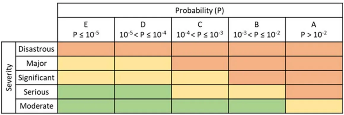
French regulation requires industrial operators to analyze technological risks using proven quantitative methods. The French Environment Ministry published, for uniformity concern, a regulatory criticality matrix (French Bulletin, 2010). Figure 1 shows this risk assessment matrix with 5x5 levels.
Figure 1: French regulatory risk matrix
This matrix defines three zones of accidental risk: high in orange, intermediate (ALARP) in yellow and minor in green. The position of accident scenarios inside this matrix makes it possible to prioritize the risk safety measures to be implemented in order to stay within the regulatory risk limits.
Paper Received: 14 January 2019; Revised: 3 April 2019; Accepted: 26 June 2019
Please cite this article as: Crija U., Olivier-Maget N., Bourgeois F., Gabas N., Iddir O., 2019, Interfacing the Probabilistic Bowtie Analysis with the Regulatory Risk Matrix, Chemical Engineering Transactions, 77, 919-924 DOI:10.3303/CET1977154
Detailed quantitative risk analysis of an undesirable event is commonly performed using the Bowtie (BT) method (. The BT combines a fault tree and an event tree that are on both sides of the undesirable or top event (Iddir, 2015). Estimating the probability of occurrence of an industrial accident involves taking into account the effect of all the prevention and mitigation barriers implemented to reduce risks. The BT analysis requires quantitative data for the frequency of occurrence of basic events. Such data is found from industrial databases and expert’s judgement. One difficulty in quantitative risk analysis lies in selecting the most relevant data for the studied case. In addition, these data are prone to uncertainties whose nature is somewhere between random or epistemic. By and large however, industrial production systems are designed, built and operated from a high level of expertise and hard data. Uncertainties associated with such a context are therefore mainly random in nature. It is thus possible to describe the occurrence probability of industrial events by a single probability distribution. This situation justifies application of a Bayesian approach to BT risk analysis, where other contexts with less information available may require risk analysis approaches capable of dealing with the lack of knowledge, such as uncertainty theories (Dubois, 2010). Finally, BT analysis should be dynamic, in that it should account for the time variation of the failure rates for the basic events of the system. Various methods have been developed to cope with these limitations (Shahriar et al., 2012; Ferdous et al., 2013; De Ruijter and Guldenmund, 2016).
The goal of our work is to propose a new way by which probabilistic BT analysis can be interfaced with the regulatory risk matrix used by decision-makers, bearing in mind that visual interpretation of risk is always a sensitive and critical issue. The work is illustrated through an industrial case study.
2. Time-dependent probabilistic bowtie model
The proposed model consists in propagating time-dependent probability distributions of occurrence of basic events through both sides of a bowtie. The aim is to obtain the occurrence probability distributions of top event and its potential consequences. Propagation of probabilities through the bowtie is achieved by Monte Carlo simulation (Vose, 1996; Vitali and Lutomski, 2004). Under the assumption that the occurrence number of an event during time period t follows a Poisson distribution, the probability of occurrence P(t) of a basic event, at time t, can be formally related to the failure rate ʎ(t) through the exponential distribution (Eq(1)).
P t =1-e-t ʎ t (1)
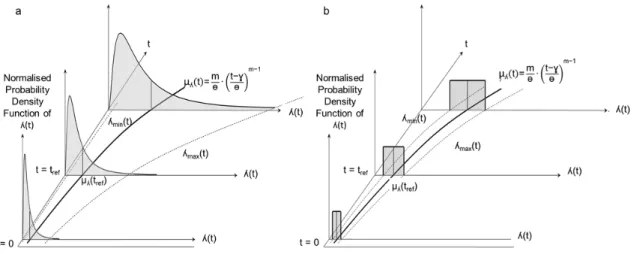
The failure rate ʎ(t) is itself a random variable, whose distribution depends on the type of event, such that P(t) is also a random variable. Typically, ʎ(t) can be described as a lognormal distribution for equipments such as pumps, valves or sensors. For other events that include human factor (e.g. operator errors) or domino effects, the uniform distribution is used instead. It is recalled that these distributions are taken here as reflecting full-fledged knowledge, which justifies the use of the Bayesian approach to BT analysis. Figure 2 shows the underlying principle of the time-dependent probabilistic model used to estimate the probability of an event at time t. Whether lognormal or uniform, it is assumed that the mean value of ʎ(t), noted μλ(t), changes with time
according to a three-parameter (m, ɵ, and ɣ) Weibull function (Teimouri and Gupta, 2013). The variance of the distribution is extrapolated assuming that the coefficient of variation stays constant. The expression of the three-parameter Weibull function is given in Figure 2.
Figure 2: Illustration of the time propagation of the probability distribution of an event (a: Lognormal distribution, b: uniform distribution)
The parameters of the probability distribution functions are derived directly from reliability tables or proprietary industrial data. Reliability databases, such as the OREDA handbook (2015), give the mean failure rate at a set reference time tref, as well as the min and max confidence bounds of the failure rate, at a specified confidence, typically 90 %. Parameters of the lognormal and uniform distributions are estimated from these values at tref. The mean and variance of the distributions are extrapolated at any operational time t using the Weibull function and the time invariance of the coefficient of variation respectively. In our model, a maintenance period can be associated to an event at which the rate of occurrence is reset to its initial value. Monte-Carlo simulation of the entire bowtie is straightforward. Random values, typically 106, of the failure rate ʎ(t) are generated for every basic BT event, for any time t of interest, say t=0.5 year, 1 year, 2 years, and so on. Each value is in turn converted into a probability of occurrence P(t) using Eq(1), yielding random values of the probability of occurrence for every basic event. These probabilities are then propagated through the bowtie using Bayesian rules (Kelly and Smith, 2009).
3. Case study
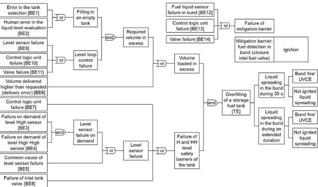
The proposed methodology is illustrated through an industrial case study provided by TechnipFMC. The corresponding bowtie is shown in Figure 3.
The top event (TE) is an "overfilling of a storage fuel tank". The fuel tank operation is secured by the following devices:
• a BPCS (Basic Process Control System) for the control of the liquid level, • two instrumented safety systems set at high and very high level respectively, • a bund,
• a hydrocarbon detector in the bund that triggers an inlet shut-off valve.
Figure 3: Bowtie of the TechnipFMC case study
The reliability data shown in Table 1 come from the OREDA database (2015) or from TechnipFMC.
Table 1: Basic events’ reliability data
Basic event (BE) Reliability data Weibull function parameters Number Distribution tref
(h) μλ(tref) per 106.h λmax(tref) per 106.h Confidence bound of λmax(tref)% m ɵ (h) ɣ (h) 1 Uniform 8760 1.14 1.71 - 1 876,002 0 2 Uniform 8760 22.83 34.24 - 1 43,800 0 3 Lognormal 24505 0.56 2.33 95 1 1,785,714 0 4 Lognormal 24505 0.56 2.33 95 1 1,785,714 0 5 Lognormal 29012 1.02 3.01 95 1 980,392 0 6 Uniform 8760 5.71 8.56 - 1 175,200 0 7 Lognormal 17520 5.22 16.25 95 1 191,571 0 8 Lognormal 26767 5.09 22.77 95 1 196,464 0 9 Lognormal 24505 0.56 2.33 95 1 1,785,714 0 10 Lognormal 17520 5.22 16.25 95 1 191,571 0 11 Lognormal 26767 5.09 22.77 95 1 196,464 0 12 Lognormal 29012 1.02 3.01 95 1 980,392 0 13 Lognormal 17520 5.22 16.25 95 1 191,571 0 14 Lognormal 26767 5.09 22.77 95 1 196,464 0 15 Uniform 8760 12.03 18.04 - 1 83,143 0
4. Results and analysis
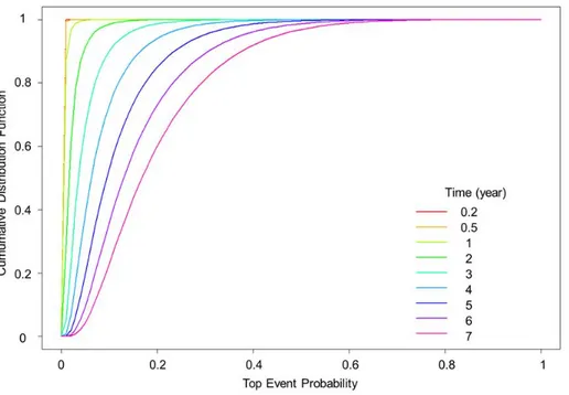
The Monte-Carlo simulation yields the probability distribution function of the probability of occurrence of BT’s top and consequence events. Figure 4 shows the cumulative distribution function (CDF) of the probability of occurrence of the top event as a function of operational time t (0.2 year ≤ t ≤ 7 years).
Figure 4: Probability distribution of the probability of occurrence of the top event
One noteworthy observation is that, based on the time propagation hypotheses used in the bowtie model, the CDF of the probability of occurrence of the top event changes over time. Moreover, the monotonic increase in spread of the distribution occurs despite the choice of Weibull’s scale parameter value m = 1 for all basic events. This is caused by the product between time t and ʎ(t) in Eq(1), which will spread the distribution of P(t)
even if the distribution of ʎ(t) is time invariant. The consequence is that the risk level of the top event, which is commonly estimated at time t = 1 year, is in fact time dependent.
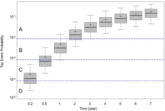
A boxplot representation of the same results is shown in Figure 5, giving a more insightful vision from a risk assessment standpoint. The boxplots show different moments and quantiles of the probability of occurrence of the top event. These include the 5 % and 95 % quantiles, the median as horizontal segments, and the mean as dots.
Figure 5: Boxplot representation of the time variation of the probability of occurrence of the top event
This graphical representation of the results is particularly effective in that it provides an easily interpretable interface between the probabilistic BT analysis and the regulatory risk assessment matrix (Figure 1). The occurrence probability of the top event is plotted on the vertical axis, and the boxplot gives a complete and effective vision of the associated distribution. As the vertical axis is plotted on a log scale, the bounds of the risk assessment matrix levels (A, B, C, D and E) can be drawn as horizontal lines on the same graph. Therefore, Figure 5 gives a direct quantification of the distribution of the risk of occurrence of the top event as a function of time. This provides an understanding of the risk associated with the top event that is rather different from the standard approach, which considers only the mean probability of occurrence. At any time t, the probability distribution of the top event spreads across all risk levels. It is noted that the mean probability of the top event, which is shown as dots in Figure 5 is precisely that obtained using a standard BT analysis based on propagation of mean event probabilities only. The spread of the boxplots show the top event likelihood or probability of belonging to individual risk matrix levels. Table 2 shows the result of the likelihood of the top event for all the times selected in Figure 5.
Table 2: Reliability data of basic events
Risk levels Time t (year)
0.2 0.5 1 2 3 4 5 6 7 A < 0.1 % 0.6 % 12.7 % 71.1 % 95.0 % 99.2 % 99.9 % 100.0 % 100.0 % B 1.8 % 42.0 % 82.1 % 28.9 % 5.0 % 0.8 % 0.1 % < 0.1 % < 0.1 % C 59.6 % 57.0 % 5.2 % < 0.1 % < 0.1 % < 0.1 % < 0.1 % < 0.1 % < 0.1 % D 38.6 % 0.4 % < 0.1 % < 0.1 % < 0.1 % < 0.1 % < 0.1 % < 0.1 % < 0.1 % E < 0.1 % < 0.1 % < 0.1 % < 0.1 % < 0.1 % < 0.1 % < 0.1 % < 0.1 % < 0.1 % Mean’s level C B B A A A A A A
Looking for example at time t = 0.5 year in Figure 5, it is apparent that the top event occurrence probability spreads mainly across the B and C risk levels. Table 2 shows that in this case 57 % of the probability lies in
the C level, 42 % in the B level, 0.6 % in the A level and 0.4 % in the D level. In other words, in terms of likelihood, this event is mainly of C level category. Its mean value lies however in the lower part of the B level (SFigure 5).
At time t = 1 year, the probability of occurrence of the top event is by and large of the B level type (Figure 5). Quantitatively, 82.1 % of the probability of occurrence lies in the B level, and the mean value is inside the B level also. However, 12.7 % of the probability of occurrence is in the A level, and 5.2 % in the C level (Table 2). The percentage that is found in the A level may give cause to pause.
As the probability distribution of occurrence is calculated for all the BT events, the same representation and analysis can be extended to any consequence events (e.g. bund fire/ UVCE, not ignited liquid spreading).
5. Conclusions and perspectives
Our research concerns the application of probabilistic bowtie analysis to the chemical industry, which has particularly comprehensive reliability databases based on datasets acquired over many decades. This permits using a purely Bayesian approach for propagating basic event probability distributions along a bowtie. Based on a bowtie model that uses time-dependent lognormal and uniform distributions, the work proposes a mode of analysis and representation that comprehensively interfaces the results of the probabilistic analysis with the risk matrix. The risk of occurrence of top and consequence events is expressed as a likelihood of belonging to a given risk level of the risk matrix. It is believed that this mode of representation may improve decision-making and help the risk management team to better identify and prioritize the actions required to reduce or maintain a desirable risk level. Coupling a sensitivity analysis to the proposed mode of analysis and representation of probabilistic bowtie results could also possibly help identify solutions that can improve the overall performance of the system with regards to safety. This could lead for example to selection of safety barriers that would guarantee that the likelihood of an undesirable event does not exceed a threshold percentage into a given risk level. Specifically, in the applicative case, this methodology could be beneficial to adjust the test interval for the safety barrier in order to guarantee a threshold percentage into a risk level. References
De Ruijter A., Guldenmund F., 2016, The bowtie method: a review, Safety science, 88, 211 – 218.
Dubois D., 2010, Representation, Propagation, and Decision Issues in Risk Analysis Under Incomplete Probabilistic Information, Risk Analysis, 30(3), 361 – 368.
French Bulletin, 2010, French bulletin of May 10th, 2010 of the French Environment Ministery, <http://www.ineris.fr/aida/consultation_document/7029#7030>.
Ferdous R., Khan F., Sadiq R., Amyotte P., Veitch B., 2013, Analyzing system safety and risks under uncertainty using a bow-tie diagram: An innovative approach, Process Safety and Environmental Protection, 91, 1 – 18.
Iddir O., 2015, Noeud papillon : une méthode de quantification du risque, Techniques de l’Ingénieur, Réf. SE 4 055.
Kelly D.L., Smith C.L., 2009, Bayesian inference in probabilistic risk assessment--The current state of the art, Reliability Engineering & System Safety, 94(2), 628 – 643.
OREDA, 2015, Offshore and onshore REliability DAta handbook, 6th edition.
Shahriar A., Sadiq R., Tesfamariam S., 2012, Risk analysis for oil & gas pipelines: A substainability assessment approach using fuzzy based bow-tie analysis, Journal of Loss Prevention in the Process Industries, 25, 505 – 523.
Teimouri M., Gupta A.K., 2013, On the Three-Parameter Weibull Distribution Shape Parameter Estimation, Journal of Data Science, 11, 403 – 414.
Vitali R., Lutomski M.G., 2004, Derivation of Failure Rates and Probability of Failures for the International Space Station Probabilistic Risk Assessment Study, in Probabilistic Safety Assessment and Management, Eds. Cornelia Spitzer, Ulrich Schmocker, Vinh N. Dang, Springer-Verlag London 2004, 1194 – 1199. Vose D., 1996, Quantitative risk analysis – A guide to Monte-Carlo simulation modelling, Wiley: New-York.