Dynamics of a slowly-varying sand bed in a circular pipe

To link to this article : DOI:

10.1016/j.ijmultiphaseflow.2016.02.007

URL :

https://doi.org/10.1016/j.ijmultiphaseflow.2016.02.007

This is an author-deposited version published in:

http://oatao.univ-toulouse.fr/

Eprints ID: 18394

O

pen

A

rchive

T

oulouse

A

rchive

O

uverte (

OATAO

)

OATAO is an open access repository that collects the work of Toulouse

researchers and makes it freely available over the web where possible.

To cite this version: Girolami, Laurence and Sherwood, John D. and

Charru, François Dynamics of a slowly-varying sand bed in a circular

pipe. (2016) International Journal of Multiphase Flow, vol. 81. pp.

113-129. ISSN 0301-9322

Any correspondence concerning this service should be sent to the repository administrator:

Dynamics

of

a

slowly-varying

sand

b

e

d

in

a

circular

pipe

L.

Girolami

a,1

_,

_J.D.

_Sherwood

b,∗

_,

_F.

_Charru

a

a IMFT, Université de Toulouse CNRS-INPT-UPS, F31400 Toulouse, France b DAMTP, University of Cambridge, Wilberforce Road, Cambridge CB3 0WA, UK

Keywords: Pipe flow Sand bed Secondary flow Stability

a

b

s

t

r

a

c

t

Thelongwave-lengthdynamicsandstabilityofabedofsandoccupyingthelowersegmentofacircular pipearestudiedanalyticallyuptofirst-orderinthesmallparametercharacterizingtheslopeofthebed. Thebedisassumedtobeatrest,withatmostathinsandlayer(thebedload)moving atthesheared interface.Whenthesandbedisplane,withdepthindependentofpositionzalongtheaxisofthepipe, thevelocityoftheliquidisknown frompreviousstudiesofstratifiedlaminarflowoftwoNewtonian liquids(thelower onewithinfiniteviscosityrepresentingthesandbed).Whenthe depthofthesand bedvarieswithz,secondaryflowsdevelopinthecross-sectional(x,y)plane,and theseare computed numerically,assumingthatthesandbedremainsastraighthorizontallineinthecross-sectionalplane. Themeanshearstressactingontheperturbedsandbedisthendeterminedbothfromthecomputed sec-ondaryflowsandbymeansoftheaveragedequationsofLuchiniandCharru.Thelatterapproachrequires knowledgeonlyoftheflowovertheunperturbed,flatsandbed,combinedwithanaccurate approxima-tionofthedistributionoftheperturbedstressesbetweenthepipewallandthesandbed.Theperturbed stressesdeterminedbythetwomethodsagreewellwitheachother.Usingthesestresses,itisthen pos-sibletoapplystandardtheoriesofbedstabilitytodeterminethebalancebetweenthedestabilizingeffect ofinertial(out-of-phase)stressesandthestabilizingeffectsofgravityandrelaxationoftheparticleflux, andvariousexamplesareconsidered.

1. Introduction

Thetransportofsand/waterslurriesalongahorizontalpipeline is of commercial importance, and has therefore been the sub-ject ofmanystudies, reviewedby e.g., PekerandHelvacı (2008); Goharzadeh etal. (2013); and Soepyan et al.(2014). The predic-tion and control of transport (or settling) of entrained sand in petroleumpipelinesissimilarlyimportant(Salama,2000).

At high fluid velocities the particles are suspended and flow withthe fluid. However, atlow velocities theparticles (if denser thanthefluid)sedimentundergravity,andastationarybedof par-ticlesformsonthelowersideofthepipe(Turianetal.,1987).Our interest hereliesinthe regime ofmoderatefluid shearstress on the bed, when particles at the bed surface are slowly entrained intoathinmovinglayer(e.g.,OroskarandTurian,1980;Takahashi andMasuyama,1991;DoronandBarnea,1995,1996;Turianetal., 1987;Peyssonetal., 2009).Thismoving layer(thebedload layer) hasathicknessofjustafewparticlediameters.

∗ _{Corresponding author. Tel.: +44 1223760436.}

1 Present address: GéHCO, Université François Rabelais de Tours, Campus Grand- mont, 37200 Tours, France

E-mail address: jds60@cam.ac.uk (J.D. Sherwood).

Manystudies haveconcentrated ontheflow ratesofthesand andwaterasfunctionsoftheappliedpressuregradient(e.g.,Doron et al., 1987; Kuru et al., 1995; Ouriemi et al., 2009a). However, a crucial issue for bedload transport is the shear stress exerted by the fluid flow over the bed: this stress determines the parti-cleflowrate.Theuppersurfaceofthebedisusuallywavy(rather than plane), so that the shear stress and particle flow rate are non-uniform inthestreamwise direction,leading tothe propaga-tion of a complex patternofsand waves,see e.g., the review by Charru etal.(2013). Thesewavesare ofboth scientific and engi-neeringinterest:ripplesanddunesareknowntohavestrong con-sequences onflow rates andpressure gradients (Takahashi etal., 1989; Takahashi andMasuyama, 1991;Ouriemi etal., 2009b; Al-Lababidietal.,2012).

Theaimofthispaperistoprovideasetofarea-averaged equa-tions governing slow variations of the fluid flow and sand bed, consistentup tofirst-orderinthesmall-slopeparameter.Wethen usetheseequationstoanalyzethelinearstability ofthebed.The analysisisrestrictedtolaminarflow,withtheusualquasistatic as-sumptionthatthetimescaleforbedheightvariationsislong com-pared to the hydrodynamictime scale, so that the flow may be calculatedasifthebedprofilewerefixed.

We first (Section 2) discuss the velocity profile and shear stresses in fluid flowing through a pipe in which the sand bed is uniform along thelength of thepipe. When the height ofthe sand bedvaries slowlyinthe axial direction, not only isthere a slowvariationintheaxialvelocityoffluidalongthepipe,but sec-ondary flows are set up in thecross-section. Such flows are dis-cussed inSection 3.InSection4we reviewastandardtheory for themovementofsandgrainsatthebedsurfaceduetothe hydro-dynamicbedstress.InSection5wederivethesetofarea-averaged equationsforthefluidflowrate,particleflowrateandbedheight, assuming that thesand flux isa function ofthe meanstress av-eraged overthewidthofthebed(the detailedstressdistribution is ignored). The equations are based on the analysis of Luchini andCharru(2010a)ofslowly-varyinglaminarflowswhichappeals to the stationarity of the viscous dissipation termin the energy equation, combined withthe approximation that theratio ofthe shearforceactingonthebedtotheshearforceactingonthe wet-ted wallof thepipe isthesame atfirst-orderasatzeroth-order. These equations, although consistent up to the first-orderin the small-slopeparameter,requireonlytheparallel-flowanalytical re-sults(i.e.,theydonotrequirethecalculationofthefirst-orderflow disturbanceovertheslowly-varyingsandbed).Thevalidityofthis analysis is confirmedby comparisonwith thefull first-order nu-mericalresultspresentedinSection3.Asanillustrationoftheuse of the area-integrated equations,a stability analysisof the plane bedisperformedinSection6.

The analysisisrestrictedto Newtonian fluids,andthereforeis inappropriate for either concentrated slurries of particles or for non-Newtonian crude petroleum: however, it is a useful starting point even for such for fluids. The Reynolds number will be re-quired to be sufficiently low for the basic flow within the pipe to be laminar,but, asis standard in longwavelength analysis of nearly parallelflow,theReynoldsnumberneednotbesmall com-paredtounity(aswillbediscussedinSection3).Theregimethat weshallinvestigateisthatinwhichparticlesatthesurfaceofthe sand bedare juststartingtomove dueto the stressimposed on thembythefluidflowingabovetheminthepipe.Thusthe analy-sisappliestoarestrictedrangeofflowrateswhichis,nevertheless, an importantone,since itseparatestheregime inwhichthebed is atrest(growing slowlyiffurtherparticles are deposited) from that in which the particlebed starts to be eroded (as would be requiredforcleaningout thepipe).Weshallre-visitthese restric-tionsinSection7,wheretheycanbemadeexplicitintermsofthe analysisofSections2–6.

2. Liquidflowthroughapipewithauniformsandbed

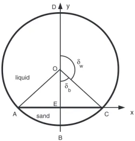
ThegeometrythatweconsiderisshowninFig.1.Thepipehas radius R.Abedofsandatthebaseofthepipesubtendsan angle 2

δ

b atthe center ofthe pipe, andhas a plane, horizontal upper

surface AEC.Theupperpartofthepipeisoccupiedbyliquid,and the portionofthecircularpipewall thatiswettedbyliquid sub-tendsanangle2

δ

w=2

(

π

−

δ

b

)

atthecenterofthepipe.

WesetupCartesiancoordinates,withzaxisparalleltotheaxis ofthepipeandwith(x,y)inthecross-sectionalplaneofthepipe. The y axisis vertical,along thesymmetry axis,andthe xaxisis horizontal, joiningthetwotriplepoints AandCwhereliquid,the pipe wallandthesandbedmeet(Fig.1).Weassume thatthe in-terfacebetweenthe sandbedandtheliquidisplane, andthatit coincides with the x axisy₌0. We shall occasionally use cylin-drical polarcoordinates(r,

ψ

,z),with

ψ

=0directedalongthey

axis.

The cross-sectional area A ofthe portion ofpipe occupied by liquidcanbefoundbyelementarymethods,andis

A₌R2

¡δ

w−1 ₂ sin2

δ

w

¢

. (1)

δ

δ

y

x

O A B C D E liquid sand w b

Fig. 1. Cross-section of the pipe, with sand at the bottom, and liquid above. The pipe has radius R and the maximum sand bed depth, EB, is h (3) . The sand bed width AEC has length C b , and the length of the wetted wall ADC is C w(2) . Inthecross-section,thelengthCbofthesandbed,andthelength

Cwoftheportionofthecylindricalwallwettedbyliquid,are

Cb=2Rsin

δ

b, Cw=2R

δ

w. (2)

Themaximumheightofthesandbed,atx₌0,is

h₌R

(

1_{− cos}

δ

b

)

=R

(

1+cos

δ

w

)

, (3)

andwenoteforfutureusethat

∂

A

∂

h =−Cb,

∂

Cb

∂

h =−2cot

δ

w. (4)

Particle velocitiesin the bedloadlayer are much smallerthan thebulkfluidvelocity,typicallyafractionofthefluidvelocityata distanceofoneparticlediameterabovethebedatrest.Henceitis usualtocalculatethefluidflowasifthewavybottomwerefixed (Charru et al., 2013), andthe errors introduced by this approxi-mationaresmall.Theliquidthereforesatisfiesano-slipboundary conditionbothatthebed/liquidinterfaceandonthecircularwall ofthepipe.

Flow of two fluidsin such a geometry hasbeen well studied (Bentwich, 1964; Ranger and Davis, 1979; Brauner et al., 1996; Biberg and Halvorsen, 2000), because of its importance when pumpingtwo fluidsthat haveseparateddueto their density dif-ference. Ifthe viscosityof thelower fluid is takento be infinite, thislowerfluidbecomesstationary,andtheflowoftheupperfluid correspondstofluidflowingaboveasandbed.Wepresentashort summaryoftheanalysisandanalyticpredictionsforthiscaseofa uniformflatbedinAppendixA.However,weshalleventuallyneed tousenumericalmethods,andit isconvenienttodoso evenfor thesimplestcaseofauniformsandbed.Theanalyticresultsthen provideausefulcheckontheaccuracyofthenumericalscheme.

The liquid is assumed to be Newtonian and incompressible, withdensity

ρ

andviscosity

η

.Ifthebedofsandisuniform, the liquidvelocitywinthezdirectionsatisfies

µ ∂

2

∂

x2 +

∂

2

∂

y2

¶

w=−G/

η

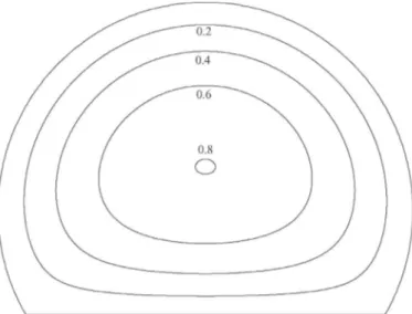
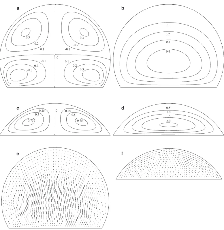
, (5)

where−G<0istheaxialpressuregradient.WesolvedthePoisson Eq.(5),subjecttoanoslipcondition attheboundaries,bymeans ofthefiniteelementpackageFreeFem++(Hecht,2012).Bywayof example,Fig.2showsisolinesofthevelocity w

(

x,y

)

,normalized byQ/R2 whereQisthevolumetricflowrate,forthecaseh/R₌0.5. Notethat themaximumvelocityisgreaterthanthevalue2/

π

for

Fig. 2. Velocity field w (x, y ) normalized by Q / R 2 where Q is the flow rate, for h/R = 0 . 5 . The FreeFem ++ calculations used 24290 triangular elements.

0 0.5 1 1.5 2 0 0.1 0.2 0.3 0.4 h/R ˆ Q

Fig. 3. Variation with h / R of the dimensionless flow rate ˆ Q = Q/ (GR4 /_{η) . ( ◦), nu-} merical solution; (—), analytical solution (7) ; (– –), asymptotic solution (115) .

Thecomputeddimensionlessflowrate

ˆ Q₌ Q GR4 /

η

, Q= Z A wdS, (6)

is shown in Fig. 3 as a function of h/R. This can be compared against the analytic result obtained by Ranger and Davis (1979), whichtakestheform

ˆ Q

(

δ

w

)

=

δ

w 8 − sin2

δ

w 24 − sin4

δ

w 96 − sin 4

δ

wI (7) where I₌ Z∞ 0

π ω

3 cosh

ωδ

wd

ω

sinh

ω

δ

wsinh2

ω

π

. (8)

DetailsaregiveninAppendixA.2,andthefiniteelement computa-tionsareaccuratetowithin0.02%.IntheAppendixitisalsoshown thattheintegralI(8)iscloselyapproximatedby

I_{≈ Ismall =} 1 6

δ

w+

δ

w 90−

δ

3 w 1890+

δ

w5 14175+· · · ,

δ

w≪

π

. (9)

Whenthisapproximationisinsertedintotheexpression(7)forQ, theerrorsare lessthan0.34%forall

δ

w.Theheighthofthesand

bedisrelatedtotheangle

δ

w bytherelation(3),andfromnowon

we shallconsiderQˆ tobea functionofh,ratherthanof

δ

w.It is

showninEq.(115)ofA.2,thatQˆ_∼

(

2− h/R

)

7 / 2 ash_→2R,ascan beseeninFig.3.

The shear stress

τ

b=

τ

yz overthe sand bedCb, andtheshear

stress

τ

w=

τ

rz over the wettedwall Cw of thecylinder, are

non-uniform. Computational results for these shear stresses, normal-ized by GR, areshown inFig. 4.Forh/R=0.25 (smallsand con-tent),thebedshearstress

τ

bvariesstrongly,withmaximumvalue

larger than 1 ₂ GR;

τ

w isnearly uniformandclosetothevalue 1 ₂ GR

(the classical value for Poiseuille flow), and decreases sharply as the sand bed is approached (

|

ψ |

.

δ

w). For higher sand content

(h/R₌1 and h/R₌1.75), both stresses are smaller than at low sandcontent,asexpected(increasingbedheightatconstant pres-suregradientcorrespondstodecreasingflowrate).

We shall later need the average shear stresses over the sand bedandwettedwall:

τ

b= 1 Cb Z Cb

τ

bdx,

τ

w= R Cw Z Cw

τ

wd

ψ

. (10)

Thesemeanshearstresses arediscussedby BibergandHalvorsen (2000)anddetailsaregiveninAppendixA.3.Inparticular,onthe sandbed,

τ

b= GR2 Cb

µ

sin2

δ

w

δ

w − sin2

δ

w 2

¶

(11) andonthewettedwall

τ

w= GR2 Cw

µ

δ

w− sin2

δ

w

δ

w

¶

. (12)

Variationswithh/Rof

τ

band

τ

w areshowninFig.5.Forh/R=0,

the classical value 1 ₂ GR is recovered. As the bed thickness in-creases, the stresses decrease (as doesthe flow rate), except for smallh/Rwhere

τ

bfirstslightlyincreases.

Themeanliquidvelocitywinthepipeis w₌Q A = 1 A Z A wdS. (13)

a

b

0 0.5 1 1.5 2 0 0.1 0.2 0.3 0.4 0.5 h/R τ / G R

Fig. 5. Variation with h / R of the mean shear stresses (10) τb ( ◦) and τw ( △ ), nor-

malised by GR . Symbols, numerical solution; (—), analytical solutions (11) and (12) .

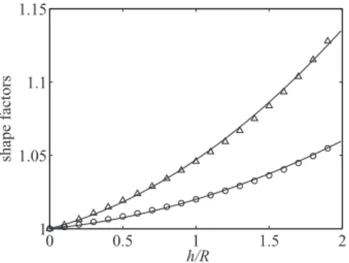
0 0.5 1 1.5 2 1 1.05 1.1 1.15 h/R shape factors

Fig. 6. Variations with h / R of the shape factors α( ◦) (14) and β ( △ ) (16) of the velocity profile w (x, y ) , normalized by αns = 4 / 3 and βns = 2 , their values for h/R = 0 . Symbols, numerical solution; (—), fits (15) and (17) .

The stability analysisof Section 6 requires theshape factor

α

of theprofileofw2 overthecrosssection,i.e.,

α

₌ 1 Aw2

Z

A

w2 dS. (14)

Results for

α

, scaled by the value

α

ns =4/3 for a pipe withno sand,areshowninFig.6asafunctionofh/R.Theyvarylittleover theentirerangeofh,andmaybeapproximatedby

α

α

ns =1+0.01

µ

h R

¶

+0.01

µ

h R

¶

2 . (15)

The end point

α

(

h₌2R

)

=35/33 can be found analytically (Ap-pendix A.5). Similarly,we shall requiretheshape factor

β

ofthe profileofw3 :

β

= 1 Aw3 Z A w3dS. (16)

Resultsfor

β

,scaledbythevalue

β

ns =2forapipewithnosand, areshowninFig.6and(likethosefor

α

)varylittleovertheentire rangeofh.Theyareapproximatedby

β

β

ns = 1 + 0.021

µ

h R

¶

+ 0.026

µ

h R

¶

2 . (17)

The end point

β

(

h₌2R

)

=490/429 can again be found analyti-cally(AppendixA.5).

3. Aslowlyvaryingsandbed

We now consider a sand bed with a height h(z) that varies slowlyasa functionoftheaxial positionz.Afirstapproximation tothefluidvelocityisgivenbythevelocitywfoundinSection2at theappropriate localvalueoftheheighthofthesandbed. How-ever, secondary flows must be established in order to allow the

fluid velocity to evolve as itmoves along the pipe. In particular, thestreamlineswillnolongerbeparalleltothepipeaxis,and in-ertialeffectsareintroduced:astandardexampleisDeanflowina helicalpipe(Bergeretal.,1983).

WefollowtheexpositionofManton(1971)whoconsidersflow throughacircularpipewithdiameterthatvariesslowlywith po-sition z along the pipe. The cross-sectional area of such a pipe changes,but notthe shape. Arelatedproblem offlow througha pipewithanellipticalcross-sectionisstudiedbyTodd(1977).The aspect ratio of the ellipseremains constant, but the ellipseaxes rotatewithpositionalong thepipe.Thus the cross-sectionalarea ofpipe remains constant, butthe shape changes.In the partially sand-filledpipe considered here, both theshape and area of the cross-sectionchangewithpositionalongthepipe.

InthisSection,we choosethepiperadius R,thevelocityW₌ Q/R2 and the stress

η

W/R as the length, velocity and pressure scales,respectively. Sincetheflowrateisconstant alongthepipe duetoincompressibility,thesescales areconstant too,unlike the pressuregradientwhichvariesslowly.Thesteadynon-dimensional Navier–Stokesequationsare

Re

(

u.

_∇

)

u=−

∇

p+

∇

2u, (18) where Re₌

ρ

RW

η

=

ρ

Q R

η

(19)

istheReynoldsnumber.

Wenowassumethatchangesinthezdirection(alongthepipe axis)occurslowlyoveralengthscaleO(R/

ǫ

),where

ǫ

≪ 1isa typ-ical bed slope. Since W₌Q/R2 is a typical fluid velocity in the axial(z) direction,velocities inthe(x,y) directionsareO(

ǫ

W) by continuity, and inertial corrections to the axial velocity field are

O(W

ǫ

Re).Thus, we follow(Manton, 1971) andseekan expansion ofthe(dimensionless)fluidvelocityandpressureintheform

u₌u(0) +h′_u(1 s ) +h′_Reu(1 i ) +· · · , (20a) p₌p(0) +h′_p(1 s ) +h′_Rep(1 i ) +· · · , (20b)

where h′_{=dh/dz is the localbed slope, u}(0) _{is the velocity in a}

uniformpipe,h′_u(1s) _{∼ O(}

_ǫ

_{)isaStokesflowcorrection dueto}

in-compressibility,andh′_Reu(1i) _{∼ O(}

_ǫ

_{Re)isthefirst inertial}

correc-tion. Thus, as is usual in problems of nearly unidirectional flow, werequireonlythat

ǫ

Re≪ 1(subject,ofcourse,totheReynolds numberbeingsufficientlysmalltoavoidtransitiontoturbulence).

The leading order solution consists of an axial flow u(0)₌

(

0,0,w(0)

₎

_,wherew

0 satisfiestheequation

∇

H2 w(0)=

∂

p(0)

∂

z , (21)

where

_∇

_H2 isthe(dimensionless)two-dimensionalLaplaceoperator

∇

H2=

∂

2

∂

x2 +

∂

2

∂

y2 . (22)

We recover here the uniform flow problem discussed in Section2,Eq.(5),whosedimensionalsolutionisgiveninAppendix A1,Eq.(104),withpressuregradientG(Q)givenby(112),or,in di-mensionlessform:

∂

p(0)

∂

z =−1/Qˆ. (23)

Inthepresentcaseofnon-uniformflow,slowvariationsofthebed heightalongthepipeimplyslowvariationsofQˆ

(

h/R

)

accordingto (7),andthereforeslowvariationsofthepressuregradient(23).

TofindtheStokesflowcorrectionu(1 s )

=

(

u(1 s )_,

_v

(1 s )_,0

₎

associ-atedwiththeslowchangesinthez-directionofthevelocityfield

Fig. 7. Isolines of the velocity gradient (h′ )−1_{∂ w} (0) /_{∂ z, normalized by Q / R} 3 , for

h/R = 0 . 5 .

w(0)_{,weshallrequirethederivative}

_∂

_w(0)_/

_∂

_{z.Onemethodto} de-termine

∂

w(0)_/

_∂

_{z wouldbetodifferentiatetheanalyticexpression} (104), holding (x, y) constant. However, the results are unwieldy, andwe againturnto numericalcomputation. Differentiating(21) withrespecttozandusing(23),wefind

∇

H2

∂

w(0)

∂

z =

∂

2 p(0)

∂

z2 = h′ ˆ Q2 dQˆ dh, (24)

wheredQˆ/dhisobtainedintermsofdI/d

δ

w bydifferentiating(7).

ThederivativedI/d

δ

wcanbeobtainedfromtheexactintegralform

(8)forI. However,forcomputational purposes itis easierto differ-entiatetheapproximateexpression(9)forI.The resulting approxi-mationfordQˆ/dhhasrelativeerrorsofatmost1.3%.Theboundary conditionsfor(24)are

1 h′

∂

w(0)

∂

z =0 onCw, (25a) =−

∂

w (0)

∂

y onCb. (25b)

Thus

∂

w(0)_/

_∂

_{z satisfies a Poisson equation (24),and could be} found by methods similar to those used in Appendix A to ob-tain w.However, we again chooseto solve (24)by means ofthe finite element package FreeFem++. Fig.7 shows

¡

h′

¢

−1

∂

w(0)_/

_∂

_z. Forpositivebedslope,theflowisaccelerated, exceptclosetothe bedwhereitslowsdown duetotheapproachofthe no-slipbed boundaryatwhichthefluidvelocityiszero.

AtO(

ǫ

),theNavier–Stokesequationsbecome

∇

H2 u(1 s )=

∂

p(1 s )

∂

x ,

∇

2 H

v

(1 s )=

∂

p(1 s )

∂

y , (26)

with incompressibility in the (x, y) plane replaced by the forced equation

∂

u(1 s )

∂

x +

∂v

(1 s )

∂

y =− 1 h′

∂

w(0)

∂

z . (27) We requireu(1 s )

=

v

(1 s )₌0on theboundary, whichis consistent

with(27)sinceincompressibilityimposesthattheintegral

Z

A

∂

w(0)

∂

z dS (28)

over the cross-sectional area A of the liquid is zero. The above equationsfortheStokescorrectionsu(1s) andp(1s) weresolved nu-merically bymeansofFreeFem++,andtypical resultsforthe ve-locitiesu(1s) and

v

(1 s )areshowninFig.8.Theverticalcomponent

v

(1 s )ispositiveandmuchlargerthanu(1s) ,sothat,forh′_>0,the

flow ispredominantlyupwards(no eddies).Close tothebed, the directionofthehorizontalStokescorrection(andshearstress) de-pends on the bedheight: forh/R < 1, thefluid pushed upwards

by therising bed(h′ _{> 0) flows into the corners,so asto move} sandgrainsfromthecenterofthebedtowardsthewalls(Fig.8a), whereasforh/R>1,thedirectionsarereversed(Fig.8c),withthe transitionbetweenthetwobehaviorsath/R₌1.

Pressure gradients in the (x, y) plane are O(

ǫ

G). The non-uniformpressure p(1s) over the(x,y)plane variesslowlyinthez

direction, leadingtoaxialpressuregradientsthatarenon-uniform over the (x, y) plane onlyat O(

ǫ

2 _{G). Theycan therefore be}

ne-glectedattheordertowhichweareworking.

Wenowconsiderinertialeffects.Inparticular,weshallrequire theinertialcorrectionw(1i)_{totheaxialvelocity,whichsatisfies}

∇

H2 w(1 i )−

∂

p(1 i )

∂

z =u (1 s )

∂

w(0)

∂

x +

v

(1 s )

∂

w(0)

∂

y + w(0) h′

∂

w(0)

∂

z (29) withboundary conditionw(1 i )_{=0on boththepipe wall andthe} surface ofthesandbed.Onceagain,incompressibilityimpliesthat the volumetric flowrate Qis fixed, andso the pressuregradient

∂

p(1i) /

∂

zin(29)mustbechoseninsuchawaythattheintegral

Z

A

w(1 i )_{dS (30)}

is zero.Aneasy wayto achievethisisfirsttosolve(29)forw(₀ 1i)

with

∂

p(1 i )_/

_∂

_{z=0,andthentocorrectthevolumetricflowrateby} pickingthepressuregradienttobe

∂

p(1 i )

∂

z = G Q R4

η

Z A w(₀ 1 i )dS₌ 1 ˆ Q Z A w(₀ 1 i )dS. (31) (As discussed above, the axial pressure gradient related to the Stokes secondary flow,

∂

p(1 s) _/

_∂

_{z, is of higher order.) The}

corre-spondingaxialvelocityis w(1i)

=w(₀ 1 i )− w(0) Z

A

w(₀ 1 i )dS. (32)

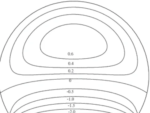
Fig.9showsatypicalvelocityfieldforw(1 i )_{.Thecorrectionis} neg-ativeinthecoreofthepipe,corresponding totheretardingeffect ofinertiainanacceleratingflow,andpositiveneartheboundaries inordertosatisfythezeronetfluxcondition.

The dimensionalshearstress onthesandbedandonthepipe wallcanbewrittenas

η

W R

¡τ

(0) +h′_Re

_τ

(1 i )

¢

=GRQˆ

¡τ

(0) +h′_Re

_τ

(1 i )

¢

(33) where

τ

(0) and

τ

(1i) are non-dimensional stresses corresponding tothenon-dimensionalvelocitiesw(0)_andw(1 i )_{.However,stresses} scaled by

η

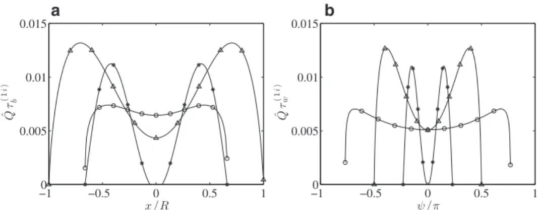
W/R₌GRQˆ becomeinfiniteasthe bedfills withsand (i.e.,ash_→2R),inthesamewayasthe non-dimensional unper-turbedpressuregradient1/Qˆbecomesinfinitewhenh→2Rwith the flow rateQ held constant.It is thereforemore convenientto discusstheinertialstressesscaledbyGR,ratherthanbyGRQˆ.This scaling,usedpreviouslyinFigs.4and5,allowsustodirectly com-paretheO(Re)stressperturbationswiththestressesinthe unper-turbedflow.

Thebedshearstress

τ

_b(1 i )varieswithpositionxacrossthebed, as doesthewall shearstress

τ

w(1 i ) onthe pipewall. These

varia-tionsareshowninFig.10forvariousvaluesofh/R,andareclearly relatedtothevariationsinaxialvelocityshowninFig.9.

Themean,scaledstressperturbation,averagedoverthesurface ofthesandbed,is

τ

(1) b = 1 Cb Z Cb

τ

(1 i ) b dx (34)

andthemean,scaledstressoverthewettedsurfaceofthepipeis

τ

(w1)= R Cw Z Cw

τ

w(1 i )d

ψ

. (35)

0.3 0.2 0.1 0 0.1 0.2 0.3 0.3 0.2 0.1 0.1 0.2 0.3 0.1 0.2 0.3 0.4 0 0.25 0.5 0.75 0.25 0.5 0.75 0.5 1.0 1.5 2.0

c

d

a

b

e

f

Fig. 8. Stokes correction to the parallel flow w (0) . (a) and (b), isolines of u (1s) and _v(1s) , for h/R = 0 . 5 ; (c) and (d), u (1s) and _v(1s) for h/R = 1 . 5 ; (e) and (f), velocity vectors

corresponding to (a,b) and (c,d).

Thesemeanstresses,togetherwiththepressuregradient

∂

p(1i) /

∂

z, areshowninFig.11.Whenthebedthicknesshissmall,theareaof thebedincreasesash3/2 :themeaninertialbedandwallstresses, and the inertial pressure gradient, are all small. When h _→ 2R

and the bed is nearly full of sand, it is shown in Eq. (148) of Appendix A.5 that the stresses

τ

(_b1) and

τ

(w1) are equal and

de-creaseas

(

2− h/R

)

1 / 2 ,whereastheperturbationpressuregradient

∂

p(1i)_/

_∂

_{z divergesas}

₍

₂

− h/R

)

−1 / 2,asshowninEq.(146).We see fromFig.11thatthereisgoodagreementbetweentheFreeFem++ numericalcomputationsoftheperturbedstressesandthe asymp-toticexpressionswhen2− h/R≪ 1.WhenFreeFem++wasusedin Section 2 to determine the fluid velocity w(0) _{above a uniform}

sand bed, we could assess the accuracy of the results by com-paring them against the analysis of Appendices A.1–A.3. In gen-eral we have no analytic results by which we might assess the accuracy of the computed inertial corrections(other than in the limit 2− h/R≪ 1). However, takingh/R₌0.5 asan example,we note that a reductionof thenumber oftriangularelements used by FreeFem++from 24290 to 6182 changed the computed iner-tialpressuregradientandmeanwallandbedstressesbylessthan 0.06%.

Finally,we considertheratioof theinertialforce onthe sand bed to the total inertial force on the bed and wetted cylinder wall,

0 0.005 0.01 0.004 0.002 0.004 0.002 0.15 0.1 0.05 0 0.025 0.05 0.075 0.1 0.1 0.075 0.05 0.025

a

b

Fig. 9. Isolines of the inertial correction w (1i) : (a), h/R = 0 . 5 ; (b), h/R = 1 . 5 .

a

b

Fig. 10. Variation in the cross-section of the pipe of the inertial shear stresses, scaled by h ′ Re GR . (a), across the bed; (b), on the pipe wall. ( ◦), h/R = 0 . 25 ; ( △ ), h/R = 1 ; ( ∗), h/R = 1 . 75 .

a

b

Fig. 11. Variations with h / R of the inertial corrections. (a) Mean shear stresses scaled by h ′ Re GR : △ , computed bed stress τ(1)

b (34) ; ◦, computed wall stress τ

(1)

w (35) ; ( −−),

asymptotic prediction (148) for δw ≪ 1 . (b) Pressure gradient ∂ p (1) / ∂ z scaled by h ′ Re G : ( −), computed (31) ; ( −−), asymptotic prediction (146) for δw ≪ 1 .

Cb

τ

_b(1)

Cb

τ

(b1)+Cw

τ

(1)

w

, (36)

andcomparethistotheratiooftheStokesforces,i.e.,by(11)and (12), Cb

τ

b(0) Cb

τ

(b0)+Cw

τ

(0) w =2sin 2

_δ

w−

δ

wsin2

δ

w 2

δ

2 w−

δ

wsin2

δ

w . (37)

Fig.12(a)showsthattheratios(36)and(37)remaincloseindeed, over the whole range of h/R. It can be seen that as h/R tends to 2,both force ratios tend to 0.5: in this limit the geometryis approaching that ofa long narrow slot,for whichwe knowthat thestressesonthetopandbottomareequal(LuchiniandCharru, 2010a),hencetheratio0.5. Thisresultisalsoconsistent withthe analytic results (130) for the unperturbed flow (A.3), and (148) fortheinertialperturbation(A.5).Amorequantitative demonstra-tionoftheclosenessoftheforceratiosisobtainedfromFig.12(b)

a

b

Fig. 12. (a) Variation with h / R of the inertial perturbed force ratio (36) ( −−), and unperturbed force ratio (37) ( −). (b) Variation with h / R of the ratio of the force ratios (38) .

whichdisplaystheratioof(36)to(37), Cb

τ

(b1) Cb

τ

b(1)+Cw

τ

(1) w Cb

τ

(b0)+Cw

τ

(0) w Cb

τ

(b0) , (38)

asafunctionofh/R.Weseethatitisclosetooneoverthewhole rangeofh/R.Thus, strikingly,theratioofthemeaninertialstress on thebedto that onthe wallcan be accurately estimatedfrom theleading-ordercalculations.

4. Sandtransport

We first review the theory of sand transport under a plane flow, i.e. for fluidflow inthe z-direction above a planesand bed

y₌0,withnovariationin thespanwisex-direction,asdiscussed by Charru et al. (2013). We assume that the sand particles are spherical, withdiameterd, density

ρ

p ,and Stokes sedimentation velocity

V_{fall =}

(

ρ

p −

ρ

)

gd

2

18

η

, (39)

wheregistheaccelerationduetogravity.

Itisknownfromexperimentthatsandparticlesonthebed sur-facedonotmoveunlesstheshearstress

τ

bactingonthebed

ex-ceedsacriticalvalue,i.e.,unless

θ

₌

τ

b

(

ρ

p−

ρ

)

gd

>

θ

t, (40)

where the dimensionless bed shear stress

θ

is known as the Shields number. Forahorizontalbed, the criticalShields number

θ

t=

θ

t0≈ 0.12 (Charruet al., 2004; Ouriemi etal., 2009a). Fora

non-zero bed slope

∂

h/

∂

z, gravity pulls thegrains downhill, and thiseffectmaybeincludedbymodifyingthecriticalShields num-berto

θ

t=

θ

t0

µ

1₊cot

(

χ

)

∂

h

∂

z

¶

, (41)

where

χ

≈ 25° istheeffectivefrictionangleofthegrains(Fredsøe, 1974).

If

θ

>

θ

t thegrainsmove,andthereisafluxqofgrainsinthe

flowingbedload(perunitlengthinthexdirection).When equilib-riumisachieved, thevolumeflux qoftheparticles(perunit bed width)saturatestoCharruetal.(2004)

qsat = ₁cq −

φ

µ π

d3 6

¶

V_fall d2

θ

(

θ

−

θ

t

)

,

θ

t<

θ

, (42a) =0, 0<

θ

<

θ

t, (42b)

withcq=0.85intheexperimentsandwheretheinclusionofthe

bed solid volume fraction

(

1−

φ

)

slightly simplifies the subse-quentequations.

Ifthe wall shear stress

τ

b variesin time or space, the

parti-clefluxq differsfromthelocalequilibriumvalue, thoughusually notby much.The relaxationofthe particlefluxtowards thenew equilibriumcanthereforebedescribedbyalinearequation Tsat

∂

_∂

q_t +Lsat

_∂

∂

q_z =qsat

(

τ

b

)

− q, (43)

wheretistime,T_sat isthe saturationtimeandL_sat the saturation length.The saturationtimescale Tsat israpid(typically1s)

com-paredto thetimescale forthegrowth ofinstabilities ofthe bed: wethereforesetthistermtozero,sothat

Lsat

∂

_∂

q_z =qsat

(

τ

b

)

− q. (44)

TheconceptofasaturationlengthLsat datesbacktoBagnold(1941, 1979)(seee.g.,Andreottietal.,2013).ThesaturationlengthLsat is poorlycharacterized.FollowingCharru(2006)weassumethatitis givenbythedepositionlength

Lsat =cL

γ

d

V_fall d, (45)

with cL=1.5 from the experiments of Charru et al. (2004) and

where

γ

is theshear rate atthe bed. Finally, mass conservation ofthelayerofmovinggrains(knownastheExnerequation)gives (forplaneflow),

∂

h

∂

t +

∂

q

∂

z=0. (46)

Forthepresent caseofpipeflow, boththeshearstress onthe bedandtheparticleflux varyinthespanwisex-direction. Never-theless,to beconsistent withthesimplificationthat theinterface betweenthesandbedandtheliquidisplane,weassumethatthe dependenceof the mean particleflux inthe z-direction, q_sat , on themeanshearstress

τ

b isstill givenby (42),i.e.,qsat=qsat

(

τ

b

)

.

Then,forpipeflow,themassconservationEq.(46)becomes

−

∂

_∂

A_t +

∂

(

_∂

C_zbq

)

=0, (47)

or,usingEqs.(2)–(4),

∂

h

∂

t +

∂

q

∂

z− h′ R cot

δ

w sin

δ

w q₌0, (48)

whereh′₌

_∂

_h/

_∂

_{z isthebedslope.The lasttermin(48)accounts} forthevariationofCb withh(or

δ

w). Notethatthistermiszero

5. Area-averagedequations

As inSection3,we nondimensionalizelengthsby R,velocities by W₌Q/R2_{,stresses by}

_η

_W/R

=

η

Q/R3_{,and time by R}3_{/Q, and}

use theReynoldsnumber Re=

ρ

WR/

η

(

19

)

.We still assume that thesurface oftheperturbed bedremainshorizontalinthe cross-sectional(x,y)plane,sothatthebedheighthisafunctiononlyof thez-coordinatealongtheaxisofthepipe.

5.1. Consistentarea-averagedequations

Averaging the conservation equations over the section of the pipe provides a useful set of simplified equations governing the slow variations of two-phase flows, see e.g., Lin and Hanratty (1986).Suchequationsarewidelyusedinengineeringapplications. However, the averaging process loses information, so that some closure lawfor theshear stress must be introduced. The closure law maybe empirical,or takenfromthe calculation ofthe first-ordercorrectionoftheleading-orderparallelflow,usingan expan-sion of the dependent variables in terms of the small-slope pa-rameter

ǫ

=h′_{. We follow here an alternative method proposed} by Luchini andCharru (2010a,2010b), which provides consistent equations (correct to first-order) without the need for full first-order calculations. However, a difficulty arises in the pipe flow considered herebecause themethod ofLuchini andCharrugives thetotal integraloftheboundary shearstressactingon thefluid butisunabletodistinguishtheseparatecontributionsofthewall andbedstresses.Theseparationofthesetwocontributionswillbe handledbyanapproximationdiscussedinSection5.2.

The equationsof continuity,axial momentum,andkinetic en-ergy, whenaveragedover thecross-sectionalarea Aoftheliquid, are

∂

A

∂

t +

∂

∂

z Z A wdS₌0, (49) Re

∂

∂

t Z A wdS₊Re

∂

∂

z Z A w2 dS₌₋ Z A

∂

p

∂

zdS− Cw

τ

w− Cb

τ

b, (50) and Re 2

∂

∂

t Z A w2 dS₊Re 2

∂

∂

z Z A w3 dS₌₋ Z A w

∂

p

∂

zdS− F, (51) where F₌₋ Z A u.

_∇

2 udS₌ Z A

(

_∇

u

)

:

(

_∇

u

)

dS (52) istherateofdissipationofenergyperunitlengthofthepipe.

Atleadingorderinthesmall-slopeparameter

ǫ

,Eqs.(49)–(51) are satisfied by uniaxial flowwith velocity w(0) _{over a sandbed} of uniformdepthh equalto thelocal beddepth,as discussedin Section 2. We now seek corrections to thisflow caused by slow

O(

ǫ

) changesinthe beddepth.Whenworkingto O(

ǫ

), itsuffices to approximatethe integrals onthe left-hand sidesof Eqs.(49)– (51) by an integral of the steady axial velocity w(0) _{at the local} beddepthhandlocalvolumetricflowrate,

w₌1 A

Z

A

w(0)_{dS (53)}

together with shapecoefficients

α

(14) and

β

(16)of the unper-turbedvelocityprofile:

α

₌ 1 Aw2 Z A

¡

w(0)

¢

2 dS,

β

₌ 1 Aw3 Z A

¡

w(0)

¢

3 dS. (54)

Note that changes in the bed height h(z, t) with time lead to changes in the local volumetric volume flow rate, so that wA is notnecessarilyequalto1.

Wesaw inSection3that

∂

p/

∂

z isafunctiononlyofz atO(

ǫ

) andisindependentof(x,y),andcanthereforebetakenoutsidethe

integrals on the right-hand sides of Eqs. (50)–(51). The averaged Eqs.(49)–(51)thereforesimplifyto

∂

A

∂

t +

∂

(

Aw

)

∂

z =0, (55) Re

∂

(

Aw

)

∂

t +Re

∂

(

α

Aw2

)

∂

z =−A

∂

p

∂

z− Cw

τ

w− Cb

τ

b, (56) and Re 2

∂

(

α

Aw2

)

∂

t + Re 2

∂

(

β

Aw3

)

∂

z =−Aw

∂

p

∂

z− F, (57) correcttoO(

ǫ

).

Anyattempttoworksolelywiththeaveragedequationsof con-tinuity (55) and momentum (56) to determine variations in the pressuregradientrequiressomesemi-empiricalclosurelawforthe shear stresses in (56), andsuch closurelaws donot usually cor-rectly capturetheO(

ǫ

) changeinthe stress.Forexample,the re-sulting dispersion relation forfree surface waves of infinitesimal amplitudeiswrong(LuchiniandCharru,2010a).Theshearstresses on our bed of sand in a pipe maybe obtained, of course, from the O(

ǫ

) calculations of Section 2. However, Luchini and Charru (2010a)showedthatifweappealtotheaveragedenergyEq.(57) in additionto theaveraged equationsofcontinuity(55) and mo-mentum (56), the equations yield the pressure gradient and to-tal shear force atthewall, correctto O(

ǫ

). The analysisrelieson the fact that therateofenergydissipation ina boundeddomain with specified boundary conditions is minimized by the Stokes flow satisfyingthe boundary conditions,so that the O(

ǫ

) pertur-bation tothe dissipationF ontherighthandside of(57) iszero. Tosee thisexplicitly, wefirstnote that

∇

2

=

∂

2

z +

∇

H2,where

∇

H2

istheLaplaceoperator inthecross-sectional(x,y)plane and

∂

z2 u

is O(

ǫ

2 ). Contributionsto F fromthe velocity components inthe cross-sectionalplane aresimilarlyO(

ǫ

2_{). Weconsideran axial}

ve-locityfieldw₌w(0)

+

δ

w,where

δ

wsatisfiestheno-slipboundary condition on thepipewallsandsandbedsurface, andhas cross-sectional averageR

A

δ

wdS=0,by (53).The dissipationF(52)can

thereforebeexpressedas F ₌ Z A

£∇

H w(0)_.

∇

Hw(0)+2

∇

H

δ

w.

∇

Hw(0)

¤

dS₊O

(

ǫ

2

)

=− Z A

£

w(0)

∇

H2 w(0)+2

δ

w

∇

H2 w(0)

¤

dS₊O

(

ǫ

2

)

=−w

∂

p (0)

∂

z +O

(

ǫ

2

₎

_{, (58)}

since

∇

H2 w(0)=

∂

p(0)/

∂

z is uniformover the cross-section ofthe

pipe. Thus,up tofirst-order,thedissipation ratedependsonlyon theleading-orderparallel-flowsolution,sothatthepressure gradi-entuptofirst-orderisprovidedbythekinetic-energyEq.(57)and theleading-orderparallelflow.

We now havethree equations (55)–(57), validto O(

ǫ

), for w,

∂

p/

∂

z andforthetotal shearforceCw

τ

w+Cb

τ

b onthe boundary

ofthefluid.However,themotionofparticlesonthesurfaceofthe bed of sand depends upon

τ

b, and not on the total shear force

Cw

τ

w+C_b

τ

b.An approximation that allows usto obtain

τ

b from

Cw

τ

w+Cb

τ

bwillbediscussedinthenextsection.

5.2. Simplifyingapproximations 5.2.1. Quasi-staticflow

A general feature of the dynamics of sand beds is that the time scale for evolution of the bedis much larger than that for changes inthe flowing fluid. The fluid flow can therefore be re-gardedasquasistatic,andalltimederivativesinthefluidequations neglected. The averaged equation ofcontinuity (55) simplifies to become

so that the volumetric flow rateis uniformalong the pipe (and equaltounitywithourchoiceofthevelocityandlengthscales).

The shape factors

α

and

β

andare well-fitted by the correla-tions (15)and(17)shown inFig. 6andvary only slowlywithh. Sincehvariesonlyslowlywithz,thevariationof

α

and

β

withz

isveryslowindeed,andcanbeneglected.Asaresult,theseshape factorscanbemovedoutsidethederivativesin(56)and(57),and when the time derivativesare neglected dueto quasi-staticflow, theseequationsbecome

Re

α

∂

w

∂

z =−A

∂

p

∂

z− Cw

τ

w− Cb

τ

b, (60)

∂

p

∂

z =

∂

p(0)

∂

z −

β

Re 2

∂

w2

∂

z . (61)

ToobtainEq.(60)atermw∂α_∂z hasbeenassumednegligiblysmall comparedto

α

∂w ∂z,whichrequires

¯

¯

¯

¯

1 A d

α

dh

¯

¯

¯

¯

≪

¯

¯

¯

¯

1

α

dA dh

¯

¯

¯

¯

=

¯

¯

¯

Cb A

¯

¯

¯

. (62)

Since theleft-hand sideof(62)istypically0.01,(seethecurvefit (15)), weseethat(62)holdsexceptwhen

δ

w∼ 0.01 andthepipe is almostfull ofsand.Theneglectofthe variationof

β

withz in (61)canbejustifiedsimilarly.NotethattheenergyEq.(61)implies thattheviscouspressuregradient

∂

p(0) /

∂

zismerelymodifiedbya Bernoulliterm,which,using(59),canbewrittenas

β

Re 2

∂

w2

∂

z =

β

Re A3

∂

A

∂

z =h′Re

∂

p(_av 1)

∂

z , (63)

where h′₌dh/dz isthelocal bedslope andwherewehaveused (4)todefine

∂

p(1) av

∂

z =−

β

A3

∂

A

∂

h =

β

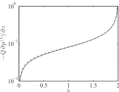
Cb A3 . (64)

The above approximations may be assessed by comparing the abovescaledpressuregradientwiththeexactfirst-order perturba-tion

∂

p(1) /

∂

z computednumericallyinSection 3.The comparison is shownin Fig. 13.Pressure gradients atconstant Q become in-finite as h _→ 2,and Fig. 13 has thereforebeen plotted to show

ˆ

Q

∂

p(av1)/

∂

zand ˆQ

∂

p(1)/

∂

z.This is equivalent to considering flow at

fixedpressuregradientratherthanatfixedvolumetricflux. We see in Fig. 13 that the pressure gradients determined via thetwo routesareallbutindistinguishable,theminordifferences originatingintheneglectofthesmallterm

∂

β

/

∂

zanduseofthe approximatecorrelations(15)and(17).

5.2.2. TheratiooftheforceCb

τ

bonthebedtotheforceCw

τ

w on

thewettedwall

EliminatingthepressuregradientinthemomentumEq.(60)by means of(61),we findthe totalshear force onthe cylinderwall andsandbed

Cw

τ

w+Cb

τ

b=−A

∂

p(0)

∂

z +Re

(

β

−

α

)

∂

w

∂

z. (65)

The firsttermon theright-hand sideof (65)istheleading-order force.Thesecondtermistheinertialcorrection,andweemphasize thatthisterminvolvesonlyleading-orderquantities.However,the area-averagedequation(65)tellsusonlyabouttheinertial correc-tion tothesumofthe forcesonthesandbedandonthewetted cylinderwall. Inaplane channel,itisknown(bysymmetry)that thechangeinstress issharedequallyoverthetopandbottom of thechannel,butherewehavenosuchsimplification.Wepropose to estimate theinertialcorrection of

τ

bby assuming thatthe

ra-tio of the forces on the bedand the wettedwall, Cb

τ

b/Cw

τ

w, is thesameastheratiooftheleadingorderforces,Cb

τ

b(0)/Cw

τ

(0) w ,as 0 0.5 1 1.5 2 10−2 10−1 100 h − ˆ Q∂ p ( 1 )/∂ z

Fig. 13. Scaled pressure gradient perturbation against bed depth h . —-, − ˆ Q∂ p (1) av /∂ z

(64) ; - - -, − ˆ Q∂ p (1) /_{∂ z computed numerically.}

Fig. 14. Scaled inertial bed stress perturbation against bed depth h . —- τ(1)

b,av(67) ; - - -, τ(1)

b computed numerically.

givenby (37).Withthisassumption,theinertialcorrection tothe bedshearstressis

h′_Re

_τ

(1) b,av=

τ

(_b0)Re

(

β

₋

α

)

Cb

τ

(b0)+Cw

τ

(0) w

∂

w

∂

z, (66)

fromwhich,using(59)and(4),wefind

τ

(_b,1_av)₌

β

−

α

A2 Cb

τ

(b0) Cb

τ

b(0)+Cw

τ

(0) w =

(

β

₋

α

)

4

(

2sin 2

_δ

w−

δ

wsin2

δ

w

)

δ

w

(

2

δ

w− sin2

δ

w

)

3 . (67) Fig.14comparestheaboveshearstress

τ

_b,(1_av ) with the exact first-ordercorrection

τ

(_b1) ascomputed numericallyinSection 3,with bothcurvesmultipliedbyQˆ asinFig.13.Theagreementis excel-lent, exceptforh< 0.5. Thisisthe rangeofh forwhichthe ap-proximationthattheratiooftheperturbed bedandwall stresses equalstheratioofthezeroth-orderbedandwallstressesis poor-est(seeFig.12).

6. Sandbeddynamicsandstability

6.1. Theequationsgoverningsandbeddynamics

We collect together here the set of area-integrated equations governingthe sand beddynamics,forslow variations ofthe bed surface. We emphasize that these equations are consistent up to O(

ǫ

) and that they involve only the leading-order, parallel flow solution ofthe full problem. The equations have been non-dimensionalizedusingthelength,velocityandstressscales intro-ducedat the beginning ofSection 5, together with the Reynolds number(19).Withinthequasistaticassumption,incompressibility (59)implies

andgivesthemeanvelocityw

(

z

)

forgivenbedprofileh(z),viathe geometric relations (1–3). The kinetic-energy equation then pro-videsthepressuregradient(61)

∂

p

∂

z =

∂

p(0)

∂

z −

β

Re 2

∂

w2

∂

z , (69)

wheretheleading-orderpressuregradient

∂

p(0)_/

_∂

_z=−1/Qˆ

₍

_δ

w

)

is

obtainedfromEqs.(7)–(9).Themomentumequationthenprovides thetotalforceonthepipewallandsandbed(65)

Cw

τ

w+Cb

τ

b=−A

∂

p(0)

∂

z +Re

(

β

−

α

)

∂

w

∂

z, (70)

with the shape coefficients

α

and

β

taken fromthe correlations (15)and(17).

Inorder topredict motionofthe sandbed, weneed toknow thestress

τ

b=

τ

(b0)+h′Re

τ

(1)

b,av actingon thebed, ratherthanthe

totalviscousforceCw

τ

w+C_b

τ

bactingonthebedandwettedpipe

wall.Butthestress

τ

(_b0)overaflatbedisknownfrom(11):

τ

(_b0)= 1 2Qˆ

(

δ

w

)

µ

sin

δ

w

δ

w − cos

δ

w

¶

, (71)

andtheapproximationdiscussedinSection5.2givesusthestress perturbation(67)duetothenon-zeroslope:

τ

(1)

b,av=

(

β

−

α

)

4

(

2sin2

δ

w−

δ

wsin2

δ

w

)

δ

w

(

2

δ

w− sin2

δ

w

)

3

. (72)

Wenow turnto theequationsgoverningtheslowtime evolu-tionofthesandbed,aspresentedinSection4.Massconservation ofthebedloadlayer(48)gives

∂

h

∂

t +

∂

q

∂

z− h′ cot

δ

w sin

δ

w q₌0, (73)

whereqisthesandfluxperunitbedwidth(non-dimensionalised byQ/R).ThisfluxobeystherelaxationEq.(44)

Lsat

∂

_∂

q_z =qsat

(

τ

b

)

− q, (74)

withthedimensionlesssaturationlength(45) Lsat=cL

τ

b

(

d/R

)

2

V_fall /W, (75)

andtheempiricalsaturatedsandflux(42) qsat q_ref =

τ

b

τ

_ref

µ τ

b

τ

_ref −

θ

t0

(

1+h′cot

χ

)

¶

, (76) where q_{ref =} cq

π

6

(

1₋

φ

)

V_fall d WR ,

τ

ref =

(

ρ

p −

ρ

)

gd

η

W/R ,

θ

t0=0.12,

χ

=25◦. (77)

An illustration of theuse of the above equations is givenin the nextsection.

6.2. Stabilityoftheflatsandbed

Theabovefluidandparticleequationsadmit asteadyand uni-formsolution,withheight h₀ ,bedshearstress

τ

0 =

τ

_b(0)

(

h₀

)

,and particlefluxq_{0 =}qsat

(

τ

0

)

.Wenowconsiderthatthisbasesolution

isperturbedsothatthebedheightisgivenbytherealpartof h₌h0 +

ǫ

h1 ei k(z−ct). (78) Themeanstressonthebedbecomes

τ

b=

τ

(b0)

(

h

)

+h′Re

τ

(1)

b,av

(

h

)

(79)

=

τ

0 +

ǫτ

1 ei k(z−ct)+higherorderterms, (80)

with

τ

_{1 =}

Ã

∂

τ

(_b0)

∂

h

¯

¯

¯

¯

¯

_Q +ikRe

τ

(_b,1_av)

!

h₁ , (81)

where thederivative of

τ

(_b0) isevaluated (ath₌h₀ )by means of the analyticresult(11),and

τ

_b,(1_av) is given by Eq.(72),again eval-uated at h₌h₀ . The corresponding saturated flux is q_{sat =}q_{0 +}

ǫ

q_sat,1 ei k(z−ct)_with

q_{sat,1 =}

∂

qsat

∂τ

b

τ

_{1 +}ikh₁

∂

qsat

∂

h′ , (82)

wherethelast termaccountsfortheeffectofgravityfornon-zero slope.Theactualsandfluxisq₌q0+

ǫ

q1eik(z−ct),with,from(74),

q1 =₁ qsat,1

+ikLsat . (83)

Finally, theparticle conservationEq.(73) givesthedimensionless complexwavevelocity

c₌q1 h₁ − q0

cot

δ

w sin

δ

w

. (84)

Withtheaboverelations,andthederivativesofqsatevaluatedfrom

(76),weobtain c q_ref /

τ

_ref = 2

τ

0 /

τ

ref −

θ

t0 1₊ikLsat

τ

1 h₁ − ik

θ

t0cot

χ

1₊ikLsat

τ

_{0 −} q0 q_ref /

τ

_ref cot

δ

w sin

δ

w , (85) whereby(77) qref

τ

ref = cq

π

108

(

1−

φ

)

µ

d R

¶

2 ≪ 1, (86)

whichissmallsincetheparticlediameterdissmallcomparedto thepiperadiusR.

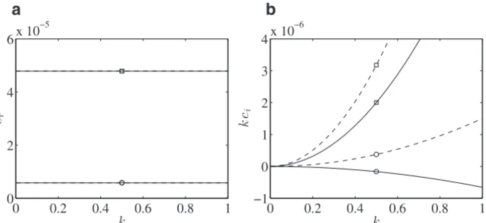
The real part c_r of c is the wave velocity (scaled by the ve-locity W₌Q/R2 ), whereas kci is the growth rate (scaled by the

time R/W). Fig. 15 displays cr and kc_i versus wavenumber, for

L_{sat =}0andthedimensionlessparametersgiveninthefigure cap-tion. Thesenumbers correspond,forexample,to apipe ofradius

R₌0.02 m, with oil flow (W₌Q/R2 ₌0.1 m/s,

ρ

=103 kg/m3 ,

µ

=0.1Pas)oversandgrains(d₌0.2mm,

ρ

p =2600kg/m3 ,cq=

0.85).Intheabsenceofthestabilizingeffectsofgravity(cot

χ

=0, dashed curves),the wave velocity isconstant (Fig. 15a), whereas the growthratekci ispositiveforall wavenumbersandincreases

quadraticallywithk(Fig.15b).(Ifhigherordertermswereincluded inthelongwavelengthexpansion,thegrowthratewould eventu-allydecreaseandbecomenegativeforhighwavenumbers(Charru, 2006).)At anygiven flow rate, the growth ratekc_i is higher for

h₌1(curves withsquares)thanforh₌0.5(curves withcircles), asexpected.Includingtheeffectofgravity(cot

χ

=2.1,solidlines) hasnoeffectonthewavevelocity,whileitsdiffusiveeffect(which scales ask2 ) simplychanges the curvature of thecurve showing thegrowthrate.Forh=0.5(curvewiththesquare),gravity stabi-lizesallwavenumbers,whereasforh₌1(curvewiththecircle),it merelydecreasesthegrowthrate.

Fig.16displays theeffectofLsat ,forh=0.5andcot

χ

=0(no gravity stabilization)andwithother parametersasinFig.15.The wave velocity (Fig. 16a) appears to be weakly affected by Lsat.

The growth rate(Fig. 16b) is moresensitive: for Lsat =0 (dashed curve), it is as in Fig. 15; for L_{sat =}0.085, it is reduced but re-mains positive (solid line); a relaxation length five times larger (i.e.,Lsat =0.425)stabilizesallwavenumbers(dashed-dottedline). TheseresultscanbeunderstoodfromEq.(85)whichgives,stillfor

a

b

Fig. 15. (a) Wave velocity scaled by Q / R 2 , and (b) growth rate scaled by Q / R 3 , for h = 0 . 5 ( ◦) and h = 1 ( ¤). - - -, cot _χ

= 0 (no gravity effect); —-, cot χ= 2 . 1 . Dimensionless parameters: h = 0 . 5 , Re = 20 , q ref = 2 . 7 × 10 −5 , θt0 = 0 . 12 and L sat = 0 . The Shields number is τ0 /τref = 0 . 31 for h = 0 . 5 , and τ0 /τref = 0 . 68 for h = 1 .

a

b

Fig. 16. (a) Wave velocity scaled by Q / R 2 , and (b) growth rate scaled by Q / R 3 , for L

sat = 0 (dashed line), L sat = 0 . 085 (solid line) and L sat = 5 × 0 . 085 (dashed-dotted line). Parameters as in Fig. 15 , with h = 0 . 5 and cot χ= 0 (no gravity effect).

cot

χ

=0, kci q_ref /

τ

_ref = 2

τ

0 /

τ

_{ref −}

θ

t0 1₊

(

kLsat

)

2

Ã

k2 Re

τ

_b,(1_av ) _{− k}2 Lsat

∂

τ

(0) b

∂

h

¯

¯

¯

¯

¯

_Q

!

. (87)

The growth rate is the sum of two terms: a positive part pro-portional to Re

τ

(_b,1_av ), arising from fluid inertia, and a negative part proportional to Lsat arising from the relaxation effect. Both terms increase monotonically with wavenumber, with the same functional dependence. Hence, Lsat does not provide any cutoff wavenumber. Such a cutoff would arise with the next order in-cluded in the long wave expansion, which would weaken the quadraticincreaseoftheinertialterm,asmentionedabove.

We have checked that use of the exact first-order bed shear stress computednumericallyinSection 3,ratherthanthe analyt-ical approximation(72),doesnot changethevelocity andgrowth rate:thecurvesinFig.16areindistinguishable.

Finally, some comparison with experimental results is appro-priate here.Letusreturntothecaseofzerogravitationaland re-laxationeffects(cot

χ

=0,Lsat =0).Thegrowthratepredictedby (85)then reduces to

kci

qref /

τ

ref =k

2_Re

₍

₂

_τ

0 /

τ

ref −

θ

t0

)

τ

(_b,1_av ). (88)

Since

τ

_b,(1_av ) >0(seeFig.14),Eq.(88)showsthatthebedisunstable assoonasthestress

τ

0=

τ

t0=

τ

ref

θ

t0andparticlesbegintomove.

At this threshold the pressure gradient is

τ

t0[

(

−

∂

p(0)/

∂

z

)

/

τ

0 ], wheretheratioofthepressuregradienttobedstressis,by(11),

−

∂

p(0)_/

_∂

_z

τ

₀ =

2

δ

w sin

δ

w−

δ

wcos

δ

w

, (89)

Fig. 17. Ratio (89) of the pressure gradient −∂ p (0) /_{∂ z and the average bed stress}

τ0 on the flat bed, against bed depth h . Squares ¤ and triangles ▽ represent scaled data from Figs. 5 and 6 of Takahashi and Masuyama (1991) .

shown in Fig. 17. For any given sand (i.e., fixed

τ

t0 ), the curve

in Fig. 17 shows (to within the constant of proportionality

τ

t0 )

the pressure gradient required to create motion of the bed of sand, as a function of the bed depth h. Also shown in Fig. 17 are scaled experimental data for the pressure gradient at which thebedbecomesunstable,takenfromFigs.5 and6ofTakahashi andMasuyama(1991).Thedatacorrespondtoparticlesofcrushed rock (diameter 2.18 mm and specific density 2.74) in pipes of diameter 2R₌49.7 mm (squares) and2R₌39.7 mm (triangles). Assuming a Shields parameter 0.066, we multiply the measured hydraulicgradientsbyfactorsof100and80,respectively,toobtain the non-dimensionaldata in Fig.17. Althoughboth experimental