Université du Québec
Institut national de la recherche scientifique (INRS) Énergie, Matériaux et Télécommunications (EMT)
Language Modeling for Speech Recognition
Incorporating Probabilistic Topic Models
A dissertation submitted in partial fulfillment of the requirements for the degree of Doctor of Philosophy
By
Md. Akmal Haidar
Evaluation Jury
External Examiner John Hershey, Mitsubishi Electric Research Laboratories
External Examiner Lidia Mangu, IBM Corporation
Internal Examiner Tiago Falk, INRS-EMT
Research Director Douglas O’Shaughnessy, INRS-EMT
Declaration
I hereby declare that except where specific reference is made to the work of others, the contents of this dissertation are original and have not been submitted in whole or in part for consideration for any other degree or qualification in this, or any other University. This dissertation is the result of my own work and includes nothing which is the outcome of work done in collaboration, except where specifically indicated in the text.
Md. Akmal Haidar 2014
Acknowledgements
I would like to express my special appreciation and thanks to my supervisor Professor Dr. Douglas O’Shaughnessy, you have been a tremendous mentor for me. I would like to thank you for encouraging my research and for allowing me to grow as a research scientist. Your wide knowledge and logical way of thinking have been of great value of me. Your under-standing, encouraging and personal guidance have provided a good basis for this thesis. Your advice on both research as well as on my career have been priceless.
I would also like to thank my committee members, Dr. Lidia Mangu, Dr. John Hershey, Professor Dr. Tiago Falk for serving as my committee members even at hardship. I also want to thank you for your brilliant comments and suggestions, thanks to you. Moreover, I would like to thank all the staffs especially Madame Hélène Sabourin, Madame Nathalie Aguiar, Mr. Sylvain Fauvel of INRS-EMT, University of Quebec, Place Bonaventure, Mon-treal, Canada, for their support in the past years. Besides, thanks goes to Dr. Mohammed Senoussaoui for helping me to write the French summary of this thesis.
A special thanks to my parents. Words cannot express how grateful I am to you for all of the sacrifices that you’ve made on my behalf. Your prayer for me was what sustained me thus far. I would also like to thank my sisters, brothers and all of my friends who supported me to strive towards my goal.
Last but not the least, thanks to almighty, the most merciful and the most passionate, for providing me the opportunity to step in the excellent research world of speech and language technology.
Abstract
The use of language models in automatic speech recognition helps to find the best next word, to increase recognition accuracy. Statistical language models (LMs) are trained on a large collection of text to automatically determine the model’s parameters. LMs encode linguistic knowledge in such a way that can be useful to process human language. Generally, a LM exploits the immediate past information only. Such models can capture short-length dependencies between words very well. However, in any language for communication, words have both semantic and syntactic importance. Most speech recognition systems are designed for a specific task and use language models that are trained from a large amount of text that is appropriate for this task. A task-specific language model will not do well for a different domain or topic. A perfect language model for speech recognition on general language is still far away. However, language models that are trained from a diverse style of language can do well, but are not perfectly suited for a certain domain. In this research, we introduce new language modeling approaches for automatic speech recognition (ASR) systems incorporating probabilistic topic models.
In the first part of the thesis, we propose three approaches for LM adaptation by cluster-ing the background traincluster-ing information into different topics incorporatcluster-ing latent Dirichlet allocation (LDA). In the first approach, a hard-clustering method is applied into LDA train-ing to form different topics. We propose an n-gram weighttrain-ing technique to form an adapted model by combining the topic models. The models are then further modified by using latent semantic marginals (LSM) using a minimum discriminant information (MDI) technique. In the second approach, we introduce a clustering technique where the background n-grams are directed into different topics using a fraction of the global count of the n-grams. Here, the probabilities of the n-grams for different topics are multiplied by the global counts of the n-grams and are used as the counts of the respective topics. We also introduce a weighting technique that outperforms the n-gram weighting technique. In the third approach, we pro-pose another clustering technique where the topic probabilities of the training documents are multiplied by the document-based n-gram counts and the products are summed up for all training documents; thereby the background n-grams are assigned into different topics.
In the second part of the thesis, we propose five topic modeling algorithms that are trained by using the expectation-maximization (EM) algorithm. A context-based proba-bilistic latent semantic analysis (CPLSA) model is proposed to overcome the limitation of a recently proposed unsmoothed bigram PLSA (UBPLSA) model. The CPLSA model can compute the correct topic probabilities of the unseen test document as it can compute all the bigram probabilities in the training phase, and thereby yields the proper bigram model for the unseen document. The CPLSA model is extended to a document-based CPLSA (DCPLSA) model where the document-based word probabilities for topics are trained. To propose the DCPLSA model, we are motivated by the fact that the words in different doc-uments can be used to describe different topics. An interpolated latent Dirichlet language model (ILDLM) is proposed to incorporate long-range semantic information by interpo-lating distance-based n-grams into a recently proposed LDLM. Similar to the LDLM and ILDLM models, we propose enhanced PLSA (EPLSA) and interpolated EPLSA (IEPLSA) models in the PLSA framework.
In the final part of the thesis, we propose two new Dirichlet class language models that are trained by using the variational Bayesian EM (VB-EM) algorithm to incorporate long-range information into a recently proposed Dirichlet class language model (DCLM). The latent variable of DCLM represents the class information of an n-gram event rather than the topic in LDA. We introduce an interpolated DCLM (IDCLM) where the class information is exploited from (n-1) previous history words of the n-grams through Dirichlet distribution using interpolated distanced n-grams. A document-based DCLM (DDCLM) is proposed where the DCLM is trained for each document using document-based n-gram events.
In all the above approaches, the adapted models are interpolated with the background model to capture the local lexical regularities. We perform experiments using the ’87-89 Wall Street Journal (WSJ) corpus incorporating a multi-pass continuous speech recognition (CSR) system. In the first pass, we use the background n-gram language model for lattice generation and then we apply the LM adaptation approaches for lattice rescoring in the sec-ond pass.
Supervisor: Douglas O’Shaughnessy, Ph.D. Title: Professor and Program Director
Contents
Contents xiii
List of Figures xix
List of Tables xxi
1 Introduction 1
1.1 Background . . . 2
1.1.1 Incorporating Long-range Dependencies . . . 4
1.1.2 Incorporating Long-range Topic Dependencies . . . 4
1.2 Overview of this Thesis . . . 6
2 Literature Review 11 2.1 Language Modeling for Speech Recognition . . . 11
2.2 Language Modeling Theory . . . 12
2.2.1 Formal Language Theory . . . 13
2.2.2 Stochastic Language Models . . . 13
2.2.3 N-gram Language Models . . . 13
2.3 Smoothing . . . 16
2.3.1 General Form of Smoothing Algorithms . . . 17
2.3.2 Witten-Bell Smoothing . . . 18
2.3.3 Kneser-Ney Smoothing . . . 19
2.3.4 Modified Kneser-Ney Smoothing . . . 20
2.4 Class-based LM . . . 20
2.5 Semantic Analysis . . . 21
2.5.1 Background . . . 21
2.5.2 LSA . . . 22
2.5.4 LDA . . . 24
2.6 Language Model Adaptation . . . 26
2.6.1 Adaptation Structure . . . 26
2.6.2 Model Interpolation . . . 27
2.6.3 MDI Adaptation Using Unigram Constraints . . . 27
2.6.4 Mixture Model Adaptation . . . 28
2.6.5 Explicit Topic Models . . . 29
2.7 Performance Measurements . . . 29
2.7.1 Perplexity . . . 29
2.7.2 Word Error Rate . . . 30
2.8 Decoding . . . 31
2.9 Experimental Tools and Data Sets . . . 34
2.10 Summary . . . 34
3 LDA-based LM Adaptation Using LSM 37 3.1 Introduction . . . 37
3.2 Mixture Language Model Using N-gram Weighting . . . 38
3.2.1 Topic Clustering . . . 38
3.2.2 Adapted Model Generation . . . 39
3.3 LM Adaptation using Latent Semantic Marginals (LSM) . . . 40
3.3.1 LSM . . . 40
3.3.2 New Adapted Model Generation Using LSM . . . 41
3.4 Experiments . . . 43
3.4.1 Data and Parameters . . . 43
3.4.2 Unsupervised LM Adaptation Using N-gram Weighting . . . 43
3.4.3 New Adapted Model Using LSM . . . 45
3.4.4 Statistical Significance and Error Analysis . . . 47
3.5 Summary . . . 48
4 Topic n-gram Count LM 51 4.1 Introduction . . . 51
4.2 LDA Training . . . 53
4.3 Topic N-gram Count Language Model . . . 53
4.3.1 Language Model Generation . . . 53
4.3.2 Language Model Adaptation . . . 54
Contents xv
4.4.1 Data and Parameters . . . 55
4.4.2 Experimental Results . . . 55
4.5 Summary . . . 57
5 Novel Topic n-gram Count LM 59 5.1 Introduction . . . 59
5.2 LDA Training . . . 60
5.3 Proposed NTNCLM . . . 61
5.4 LM Adaptation Approach . . . 62
5.5 Experiments . . . 63
5.5.1 Data and Parameters . . . 63
5.5.2 Experimental Results . . . 63
5.6 Summary . . . 65
6 Context-based PLSA and Document-based CPLSA 67 6.1 Introduction . . . 67
6.2 Review of PLSA and UBPLSA Models . . . 68
6.2.1 PLSA Model . . . 68
6.2.2 UBPLSA Model . . . 69
6.3 Proposed CPLSA Model . . . 70
6.4 Proposed DCPLSA Model . . . 72
6.5 Parameter Estimation of the DCPLSA Model Using the EM Algorithm . . . 73
6.6 N-gram Probabilities of the Test Document . . . 76
6.7 Comparison of UBPLSA, CPLSA and DCPLSA Models . . . 77
6.8 Complexity Analysis of the UBPLSA, CPLSA and DCPLSA Models . . . 77
6.9 Experiments . . . 78
6.9.1 Data and Parameters . . . 78
6.9.2 Experimental Results . . . 78 6.10 Summary . . . 80 7 Interpolated LDLM 83 7.1 Introduction . . . 83 7.2 LDLM . . . 84 7.3 Proposed ILDLM . . . 85
7.4 Incorporating Cache Models into LDLM and ILDLM Models . . . 87
7.5.1 Data and Parameters . . . 89
7.5.2 Experimental Results . . . 89
7.6 Summary . . . 90
8 Enhanced PLSA and Interpolated EPLSA 93 8.1 Introduction . . . 93
8.2 Proposed EPLSA and IEPLSA Models . . . 94
8.2.1 EPLSA . . . 94
8.2.2 IEPLSA . . . 95
8.3 Comparison of PLSA, PLSA Bigram and EPLSA/IEPLSA . . . 96
8.4 Incorporating the Cache Model Through Unigram Scaling . . . 96
8.5 Experiments . . . 98
8.5.1 Data and Parameters . . . 98
8.5.2 Experimental Results . . . 98 8.6 Summary . . . 100 9 Interpolated DCLM 103 9.1 Introduction . . . 103 9.2 DCLM . . . 104 9.3 Proposed IDCLM . . . 106
9.4 Comparison of DCLM and IDCLM Models . . . 109
9.5 Experiments . . . 109
9.5.1 Data and Parameters . . . 109
9.5.2 Experimental Results . . . 110
9.6 Summary . . . 111
10 Document-based DCLM 113 10.1 Introduction . . . 113
10.2 Proposed DDCLM . . . 114
10.3 Comparison of DCLM and DDCLM Models . . . 117
10.4 Experiments . . . 117
10.4.1 Data and Parameters . . . 117
10.4.2 Experimental Results . . . 118
Contents xvii
11 Conclusion and Future Work 121
11.1 Contributions . . . 121
11.2 Summary of the Experimental Results . . . 124
11.3 Future Work . . . 126
12 Résumé en français 129 12.1 Introduction . . . 129
12.1.1 La modélisation de la langue pour la reconnaissance vocale . . . . 129
12.1.2 Outils expérimentaux et les bases de données . . . 130
12.1.3 Contributions . . . 131
12.2 Adaptation LM en utilisant LDA . . . 131
12.2.1 Adaptation LM à base de LDA en utilisant la Sémantique latente marginale (LSM) . . . 131
12.2.2 Sujet n-gramme compte LM (TNCLM) . . . 136
12.2.3 Nouveau compte de n-gramme du sujet du LM . . . 137
12.3 Cinq nouveaux modèles probabilistes du sujet . . . 139
12.3.1 PLSA LM basée sur le contexte . . . 140
12.3.2 La LDLM interpolée . . . 143
12.3.3 La PLSA améliorée et EPLSA l’interpolée . . . 144
12.4 Deux nouvelles approches de DCLM . . . 146
12.4.1 La DCLM interpolée . . . 147
12.4.2 DCLM à base du document . . . 149
12.5 Conclusion . . . 152
12.5.1 Principales contributions de la thèse . . . 152
References 155
List of Figures
2.1 Speech recognition system . . . 12
2.2 Graphical structure of the PLSA model. The shaded circle represents ob-served variable. . . 23
2.3 Graphical model representation of LDA. The shaded circle represents ob-served variable. . . 25
2.4 General structure of SLM adaptation . . . 27
2.5 A typical speech recognition system . . . 31
2.6 Fragment of decoder network . . . 32
2.7 Early application of language models . . . 33
3.1 Topic clustering and LM adaptation using n-gram weighting . . . 39
3.2 New adapted model generation Using LSM . . . 42
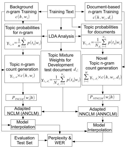
4.1 Topic n-gram count LM Adaptation . . . 52
4.2 WER results (%) for the ANCLM model developed by using confidence measure P(wi|tk) . . . 57
4.3 WER results (%) for the ANCLM model developed by using confidence measure P(tk|wi) . . . 58
5.1 Adaptation of TNCLM and NTNCLM . . . 61
5.2 WER results (%) of the language models . . . 65
6.1 Matrix decomposition of the CPLSA model . . . 71
6.2 Matrix decomposition of the DCPLSA model . . . 72
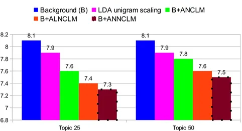
6.3 WER results (%) for different topic sizes . . . 80
7.1 The graphical model of the LDLM. Shaded circles represent observed vari-ables. . . 85
8.1 The graphical model of the EPLSA model. The shaded circle represents the observed variables. H and V describe the number of histories and the size
of vocabulary. . . 94
8.2 WER Results (%) of the Language Models . . . 100
9.1 The graphical model of the DCLM. Shaded circles represent observed vari-ables. . . 105
9.2 The graphical model of the IDCLM. Shaded circles represent observed vari-ables. . . 106
9.3 WER results (%) for different class sizes . . . 110
10.1 The graphical model of the DDCLM. Shaded circles represent observed variables. . . 114
10.2 WER results (%) for different class sizes . . . 119
12.1 Système de reconnaissance vocale . . . 130
12.2 Résultats WER (%) sur les données de test Novembre 1993 pour le modèle de ANCLM développé en utilisant la mesure de la confiance P(wi|tk) . . . . 138
12.3 Résultats WER (%) sur les données de test Novembre 1993 pour le modèle de ANCLM développé en utilisant la mesure de la confiance P(tk|wi) . . . . 139
12.4 Résultats tels que mesurés par le WER (%) obtenus sur les données de test Novembre 1993 à l’aide des modèles de langage . . . 140
12.5 Résultats tels que mesurés par le WER (%) des modèles de langue . . . 143
12.6 Résultats tels que mesurés par le WER (%) des modèles de langue . . . 145
12.7 Résultats tels que mesurés par le WER (%) des modèles de langue . . . 147
12.8 Résultats tels que mesurés par le WER (%) pour différentes tailles des classes149 12.9 Résultats WER (%) pour la taille des classes différentes . . . 152
List of Tables
3.1 Perplexity results of the tri-gram language models using n-gram weighting on November 1993 test data . . . 43 3.2 Perplexity results of the tri-gram language models using n-gram weighting
on November 1992 test data . . . 44 3.3 WER results (%) of the tri-gram language models using n-gram weighting
on November 1993 test data . . . 44 3.4 WER results (%) of the tri-gram language models using n-gram weighting
on November 1992 test data . . . 44 3.5 Perplexity results on the November 1993 test data using tri-gram language
models obtained by using LSM . . . 45 3.6 Perplexity results on the November 1992 test data using tri-gram language
models obtained by using LSM . . . 45 3.7 WER results (%) on the November 1993 test data using tri-gram language
models obtained by using LSM . . . 46 3.8 WER results (%) on the November 1992 test data using tri-gram language
models obtained by using LSM . . . 46 3.9 For the November 1993 test set using topic size 25 and the ’87-89 corpus,
ASR results for deletion (D), substitution (S), and insertion (I) errors, and also the correctness (Corr) and accuracy (Acc) of the tri-gram language models 48 3.10 For the November 1992 test set using topic size 75 and the ’87-89 corpus,
ASR results for deletion (D), substitution (S), and insertion (I) errors, and also the correctness (Corr) and accuracy (Acc) of the tri-gram language models 48 4.1 Perplexity results of the ANCLM model generated using the confidence
measure P(wi|tk) for the hard and soft clustering of background n-grams . . 55
4.2 Perplexity results of the ANCLM model generated using the confidence measure P(tk|wi) for the hard and soft clustering of background n-grams . . 56
5.1 Perplexity results of the language models . . . 64 6.1 Perplexity results of the topic models . . . 79 6.2 p-values obtained from the paired t test on the perplexity results . . . 79 6.3 p-values obtained from the paired t test on the WER results . . . 80 7.1 Distanced n-grams for the phrase “Speech in Life Sciences and Human
So-cieties” . . . 86 7.2 Perplexity results of the language models . . . 90 8.1 Distanced n-grams for the phrase “Speech in Life Sciences and Human
So-cieties” . . . 96 8.2 Perplexity results of the language models . . . 99 9.1 Distanced tri-grams for the phrase “Interpolated Dirichlet Class Language
Model for Speech Recognition” . . . 107 9.2 Perplexity results of the models . . . 110 9.3 p-values obtained from the match-pair test on the WER results . . . 111 10.1 Perplexity results of the models . . . 118 10.2 p-values obtained from the paired t test on the perplexity results . . . 119 10.3 p-values obtained from the paired t test on the WER results . . . 119 12.1 Résultats tels que mesurés par la perplexité des modèles de langage
tri-gramme utilisant la pondération n-tri-gramme sur les Caractéristiques de test Novembre 1993 . . . 133 12.2 Résultats tels que mesurés par la perplexité des modèles de langage
tri-gramme utilisant la pondération n-tri-gramme sur les données de test Novem-bre 1992 . . . 133 12.3 Résultats WER (%) des modèles de langage à l’aide de pondération
tri-gramme sur les données de test Novembre 1993 . . . 133 12.4 Résultats tels que mesurés par le WER (%) des modèles de langage à l’aide
de pondération tri-gramme sur les données de test Novembre 1992 . . . 133 12.5 Résultats tels que mesurés par la perplexité sur les données du test
Novem-bre 1993 à l’aide de modèles de langage tri-gramme obtenus en utilisant la LSM . . . 134
List of Tables xxiii
12.6 Résultats tels que mesurés par la perplexité sur les données du test Novem-bre 1992, utilisant des modèles de langage tri-gramme obtenus en utilisant la LSM . . . 134 12.7 Résultats tels que mesurés par le WER (%) sur les données du test
Novem-bre 1993 à l’aide des modèles de langage tri-gramme obtenus en utilisant LSM. . . 135 12.8 Résultats tels que mesurés par le WER (%) sur les données du test
Novem-bre 1992, utilisant des modèles de langage tri-gramme obtenus en utilisant LSM. . . 135 12.9 Résultats tels que mesurés par l’ASR pour les erreurs de la suppression (D),
la substitution (S), et l’insertion (I), et aussi pour l’exactitude (Corr) et la précision (Acc), des modèles de langage tri-gramme obtenus en utilisant l’ensemble du test Novembre 1993 avec la taille du sujet 25 et le corpus 87-89. . . 136 12.10Résultats tels que mesurés par l’ASR pour les erreurs de la suppression (D),
la substitution (S), et l’insertion (I), et aussi pour l’exactitude (Corr) et la précision (Acc), des modèles de langage tri-gramme obtenus en utilisant l’ensemble du test Novembre 1992 avec la taille du sujet 75 et le corpus 87-89. . . 136 12.11Résultats de la perplexité des données de test Novembre 1993 en utilisant
le modèle de ANCLM généré en utilisant la mesure de confiance P(wi|tk)
pour les regroupements durs et mous de n-grammes de fond. . . 137 12.12Résultats de la perplexité des données de test Novembre 1993 en utilisant
le modèle de ANCLM généré en utilisant la mesure de confiance P(tk|wi)
pour les regroupements durs et mous de n-grammes de fond. . . 138 12.13Résultats tels que mesurés par la perplexité obtenus sur les données de test
Novembre 1993 en utilisant le trigramme du langage modèles. . . 140 12.14Résultats de la perplexité des modèles sujets . . . 142 12.15 p-valeurs obtenues à partir de la t test apparié sur les résultats de la perplexité142 12.16 p-valeurs obtenues à partir de la t test apparié sur les résultats WER . . . . 143 12.17Résultats tels que mesurés par la perplexité des modèles de langage . . . . 145 12.18Résultats tels que mesurés par la perplexité des modèles de langage . . . . 146 12.19Résultats tels que mesurés par la perplexité des modèles . . . 148 12.20Valeurs p obtenues à partir des essais des paires-identifiées sur des résultats
12.21Résultats de la perplexité des modèles . . . 151 12.22 p-valeurs obtenues à partir de la t test apparié sur les résultats de la perplexité151 12.23 p-valeurs obtenues à partir de la t test apparié sur les résultats WER . . . . 151
Chapter 1
Introduction
The primary means of communication between people is speech. It has been and will be the dominant mode of human social bonding and information exchange from human creation to the new media of future. Human beings have envisioned to communicate with machines via natural language long before the advancement of computers. Over the last few decades, research in automatic speech recognition has attracted a great deal of attention, which con-stitutes an important part in fulfilling this vision.
In our daily life, we may find many real applications of automatic speech recognition (ASR). For example, in most of the latest cellular phones, especially smartphones, ASR functions are available to do simple tasks such as dialing a phone number, writing a message, or to run an application using voice instead of typing. An automotive navigation system with ASR capability can be found inside cars, which let the driver to focus on driving while controlling the navigation system through voice. Besides, there are many applications of ASR systems that perform advanced tasks such as dictation. Those are just a few examples that describe how the ASRs bring a real value on the daily life [79].
Early stages of ASR systems were based on template-matching techniques. Template-matching refers to the incoming speech signal being compared to a set reference patterns, or templates. The first known template-based ASR system was developed by Davis et al. [25] in 1952. That was a very simple task, which was to recognize a digit (isolated words) from a speaker. Ever since, many small vocabulary (order of 10-100 words) ASR tasks were carried out by several researchers. In the 1970’s, significant developments in ASR research began where the size of vocabulary was increasing to a medium size (100-1000 words), with continuous words and these methods were using a simple template-based pattern recogni-tion. In 1980’s, the vocabulary size of ASR was further increasing from medium to a large vocabulary size (> 1000 words) and the method was shifted from a template-based approach
to a statistical modeling framework, most notably the hidden Markov model (HMM) frame-work [31, 79]. In the large vocabulary ASR systems, potential confusion increases between similar sounding words. An ASR system concentrating on the grammar structure (language model) of the language was proposed by Jelinek et al. [62], where the language model was represented by statistical rules that can distinguish similar sounding words and can tell which sequence (phonemes or words) that is likely to appear in the speech.
Language modeling is the challenge to capture, characterize and exploit the regularities of natural language. It encodes the linguistic knowledge that is useful for computer systems when dealing with human language. Language modeling is critical to many applications that process human language with less than complete knowledge [28]. It is widely used in a variety of natural language processing tasks such as speech recognition [6, 57], hand-written recognition [74], machine translation [17], and information retrieval [86]. However, one of the most exciting applications of language models is in automatic speech recognition (ASR), where a computer is used to transcribe the spoken text into written form. An ASR system consists of two components: the acoustic model and the language model (LM). The LM combines with the acoustic model to reduce the acoustic search space and resolve the acoustic ambiguity. It not only helps to disambiguate among acoustically similar phrases such as (for, four, fore) and (recognize speech, wreck a nice beach), but also guides the search for the best acoustically matching word sequence towards ones with the highest lan-guage probabilities [55]. ASR systems cannot find the correct word sequence without a LM. They provide a natural way of communication between human and machine as if they were speaking as humans using natural language.
1.1
Background
There is a great deal of variability in natural language. Natural language grammar can be taught by two approaches: rule-based language models and statistical language models. In rule-based language models, grammar is defined as a set of rules that are accurate, but difficult to learn automatically. These rules are manually created by some experts such as linguists. In this approach, a sentence is accepted or rejected based on the set of rules defined in the grammar. This approach may be useful for a small task, where the rules for all possibilities of sentences can be defined. However, in natural language, there are more chances for the sentences to be ungrammatical. Statistical language models are useful to model natural language by creating several hypothesis for a sentence. They can model the language grammar by a set of parameters, which can learn automatically from a reasonable
1.1 Background 3
amount of training data. Therefore, it can save more time as the parameters can be learned automatically.
The most powerful statistical models are the n-gram models [61, 63, 75]. These models exploit the short-range dependencies between words in a language very well. To learn its parameters (n-gram probabilities) from a given corpus, the n-gram models use maximum likelihood (ML) estimation. However, n-gram models suffer from the data sparseness prob-lem as many n-grams do not appear in a training corpus, even with a large amount of training corpus. For example, if we use a vocabulary V of size 10,000 words in a trigram model, the total number of probabilities to be estimated is |V |3 = 1012. For any training data of manageable size, many of the probabilities will be zero. The data sparseness problem is also caused by the n-grams with low frequency of occurrences in a large training corpus that will have an unreliable probability.
To deal with the data sparseness problem, a smoothing technique is considered that en-sures some probabilities (>0) to the words that do not appear (or appear with low frequency) in a training corpus. The idea of smoothing is to take out some probability mass from the seen events and distribute it to the unseen events. The method can be categorized depending on how the probability mass is taken out (discounting) and how it is redistributed (back-off). Examples of some smoothing techniques are additive smoothing [70], Good-Touring estimate [36], Jelinek-Mercer smoothing [61], Katz smoothing [64], Witten-Bell smooth-ing [9], absolute discountsmooth-ing [81], and Kneser-Ney smoothsmooth-ing [66]. The details of them can be found in [19].
Class-based n-gram LMs [16] have also been proposed to solve the data sparseness problem. Here, multiple words are grouped into a word class, and the transition probabili-ties between words are approximated by the probabiliprobabili-ties between word classes. However, class-based n-grams work better only with a limited amount of training data with fewer parameters than in the word n-gram model [16]. The class-based n-gram LM is improved by interpolating with a word-based n-gram LM [15, 99]. A word-to-class backoff [83] was introduced where a class-based n-gram LM is used to predict unseen events, while the word-based n-gram LM is used to predict seen events. However, when the class-based and word-based LMs are used together, the parameter size increases more than the independent case, which is not good for low resource applications [80]. In [103], multi-dimensional word classes were introduced to improve the class-based n-grams. Here, the classes represent the left and right context Markovian dependencies separately. A back-off hierarchical class-based LM was introduced to model unseen events using the class models in various layers of a clustering tree [106]. In [18], a new class-based LM called Model M was introduced
by identifying back-off features that can improve test performance by reducing the size of a model. Here, the n-gram features were shrunken for n-grams that differ only in their his-tories. Unsupervised class-based language models such as Random Forest LM [102] have been investigated that outperform a word-based LM.
The neural network language model (NNLM) was also investigated to tackle the data sparseness problem by learning distributed representation of words [12, 90]. Here, the (n − 1) history words are first mapped into a continuous space and then the n-gram probabilities given the history words are estimated. Later, a recurrent neural network-based LM was investigated that shows better results than NNLM [76, 77].
1.1.1
Incorporating Long-range Dependencies
The improvement of n-gram models can fall into two categories, whether one is introducing a better smoothing method or incorporating long-range dependencies. Statistical n-gram LMs suffer from shortages of long-range information, which limit performance. They use the local context information by modeling text as a Markovian sequence and capture only the local dependencies between words. They cannot capture the long-range information of natural language. Several methods have been investigated to overcome this weakness. A cache-based language model is an earlier approach that is based on the idea that if a word appeared previously in a document it is more likely to occur again. It helps to increase the probability of previously observed words in a document when predicting a future word [69]. This idea is used to increase the probability of unobserved but topically related words, for example, trigger-based LM adaptation using a maximum entropy framework [88]. However, the training time requirements (finding related word pairs) of this approach are computation-ally expensive.
1.1.2
Incorporating Long-range Topic Dependencies
Language models perform well when the test environment matches nicely with the training environment. Otherwise, adaptation for the test set is essential because the smoothing ap-proaches do not consider the issues such as topic and style mismatch between the training and test data. Actually, it is impossible to collect all forms of topics and styles of a language in the training set. So, in most cases of practical tasks, adaptation of a language model is required. Many approaches have been investigated to capture the topic related long-range dependencies. The first technique was introduced in [67] using a topic mixture model. Here, topic-specific language models are trained using different corpora with different
top-1.1 Background 5
ics and combined in a linear way. Another well-known method is the sentence-level mixture models, which create topic clusters by using a hard-clustering method where a single topic is assigned to each document and used in LM adaptation. Improvements were shown both in perplexity and recognition accuracy over an unadapted trigram model [58].
Recently, various techniques such as Latent Semantic Analysis (LSA) [10, 26], Proba-bilistic LSA (PLSA) [33, 54], and Latent Dirichlet Allocation (LDA) [13] have been inves-tigated to extract the latent topic information from a training corpus. All of these methods are based on a bag-of-words assumption, i.e., the word-order in a document can be ignored. These methods have been used successfully for speech recognition [10, 33, 39, 72, 73, 78, 80, 95, 96]. In LSA, a word-document matrix is used to extract the semantic information. In PLSA, each document is modeled by its own mixture weights and there is no generative model for these weights. So, the number of parameters grows linearly when increasing the number of documents, which leads to an overfitting problem. Also, there is no method to assign probability for a document outside the training set. On the contrary, the LDA model was introduced where a Dirichlet distribution is applied on the topic mixture weights cor-responding to the documents in the corpus. Therefore, the number of model parameters is dependent only on the number of topic mixtures and the vocabulary size. Thus, LDA is less prone to overfitting and can be used to compute the probabilities of unobserved test docu-ments. However, the LDA model can be viewed as a set of unigram latent topic models. The LDA model is one of the most widely used topic-modeling methods used in speech recognition that capture long-distance information through a mixture of unigram topic dis-tributions. In the idea of an unsupervised language model adaptation approach, the unigram models extracted by LDA are adapted with proper mixture weights and interpolated with the n-gram baseline model [95]. To extend the unigram bag-of-words models to n-gram models, a hard-clustering method was employed on LDA analysis to create topic models for mixture model adaptation and showed improvement in perplexity and recognition accuracy [72, 73]. Here, the mixture weights of the topic clusters are created using the latent topic word counts obtained from the LDA analysis. A unigram count weighting approach [39] for the topics generated by hard-clustering has shown better performance over the weighting approach described in [72, 73]. LDA is also used as a clustering algorithm to cluster training data into topics [51, 87]. The LDA model can be merged with n-gram models and achieve perplexity reduction [91]. A non-stationary version of LDA can be developed for LM adaptation in speech recognition [22]. The LDA model is extended by HMM-LDA to separate the syn-tactic words from the topic-dependent content words in the semantic class, where content words are modeled as a mixture of topic distributions [14]. Style and topic language model
adaptation are investigated by using context-dependent labels of HMM-LDA [56]. A bigram LDA topic model, where the word probabilities are conditioned on their preceding context and the topic probabilities are conditioned on the documents, has been recently investi-gated [100]. A similar model but in the PLSA framework called a bigram PLSA model was introduced recently [82]. An updated bigram PLSA model (UBPLSA) was proposed in [7] where the topic is further conditioned on the bigram history context. A topic-dependent LM, called topic dependent class (TDC) based n-gram LM, was proposed in [80], where the topic is decided in an unsupervised manner. Here, the LSA method was used to reveal latent topic information from noun-noun relations [80].
Although the LDA model has been used successfully in recent research work for LM adaptation, the extracted topic information is not directly useful for speech recognition, where the latent topic of n-gram events should be of concern. In [20], a latent Dirichlet language model (LDLM) was developed where the latent topic information was exploited from (n-1) history words through the Dirichlet distribution in calculating the n-gram prob-abilities. A topic cache language model was proposed where the topic information was obtained from long-distance history through multinomial distributions [21]. A Dirichlet class language model (DCLM) was introduced in [21] where the latent class information was exploited from the (n-1) history words through the Dirichlet distribution in calculat-ing the n-gram probabilities. The latent topic variable in DCLM reflects the class of an n-gram event rather than the topic in the LDA model, which is extracted from large-span documents [21].
1.2
Overview of this Thesis
We began this thesis by stating the importance of language modeling for automatic speech recognition. The history of language modeling is then stated followed by the improvement of LMs incorporating smoothing algorithms and long-range dependencies. The remainder of this thesis is organized into the following chapters:
Chapter 2: Literature Review
In this chapter, we illustrate the basics of language modeling in speech recognition, lan-guage modeling theory, n-gram lanlan-guage models, the lanlan-guage model’s quality measure-ment metrics, the importance of smoothing algorithms, the class-based language model, the language model adaptation techniques, and semantic analysis approaches.
1.2 Overview of this Thesis 7
Chapter 3: LDA-based LM Adaptation Using LSM
We form topics by applying a hard-clustering method into the document-topic matrix of the LDA analysis. Topic-specific n-gram LMs are created. We introduce an n-gram weighting approach [40] to adapt the component topic models. The adapted model is then interpo-lated with a background model to capture local lexical regularities. The above models are further modified [49] by applying an unigram scaling technique [68] using latent semantic marginals (LSM) [96].
Chapter 4: Topic n-gram Count LM
We propose a topic n-gram count LM (TNCLM) [42] using the features of the LDA model. We assign background grams into topics with counts such that the total count of an n-gram for all topics is equal to the global count of the n-n-grams. Here, the topic weights for the n-gram are multiplied by the global count of the n-grams in the training set. We apply hard and soft clustering of the background n-grams using two confidence measures: the probability of word given topic and the probability of topic given word. The topic weights of the n-gram are computed by averaging the confidence measures over the words in the n-grams.
Chapter 5: Novel Topic n-gram Count LM
The TNCLM model does not capture the long-range information outside of the n-gram events. To tackle this problem, we introduce a novel topic n-gram count language model (NTNCLM) using document-based topic distributions and document-based n-gram counts [48].
Chapter 6: Context-based PLSA and Document-based CPLSA
We introduce a context-based PLSA (CPLSA) model [43], which is similar to the PLSA model except the topic is conditioned on the immediate history context and the document. We compare the CPLSA model with a recently proposed unsmoothed bigram PLSA (UB-PLSA) model [7], which can calculate only the seen bigram probabilities that give the incor-rect topic probability for the present history context of the unseen document. An extension of the CPLSA model defined as the document-based CPLSA (DCPLSA) model is also
in-troduced where the document-based word probabilities for topics are trained in the CPLSA model [50].
Chapter 7: Interpolated LDLM
Since the latent Dirichlet LM (LDLM) model [20] does not capture the long-range informa-tion from outside of n-gram events, we present an interpolated LDLM (ILDLM) by using different distanced n-grams [44]. We also incorporate a cache-based LM into the above models, which model the re-occurring words, through unigram scaling to adapt the LDLM and ILDLM models that model the topical words.
Chapter 8: Enhanced PLSA and Interpolated EPLSA
Similar to the LDLM and ILDLM approaches, we introduce an enhanced PLSA (EPLSA) and an interpolated EPLSA (IEPLSA) model in the PLSA framework. Default background n-grams and interpolated distanced n-grams are used to derive EPLSA and IEPLSA mod-els [45]. A cache-based LM that modmod-els the re-occurring words is also incorporated through unigram scaling to the EPLSA and IEPLSA models, which models the topical words.
Chapter 9: Interpolated DCLM
The Dirichlet class LM (DCLM) model [21] does not capture the long-range information from outside of the n-gram window that can improve the language modeling performance. We present an interpolated DCLM (IDCLM) by using different distanced n-grams [47].
Chapter 10: Document-based DCLM
We introduce a document-based DCLM (DDCLM) by using document-based n-gram events. In this model, the class is conditioned on the immediate history context and the document in the original DCLM model [21] where the class information is obtained from the (n-1) history words of background n-grams. The counts of the background n-grams are the sum of the n-grams in different documents where they could appear to describe different topics. We consider this problem in the DCLM model and propose the DDCLM model [46].
1.2 Overview of this Thesis 9
We summarize the proposed techniques and the possible future work, where our proposed approach could be considered.
Chapter 2
Literature Review
In this chapter, we describe the foundation of other chapters. We first review the basic uses of language models in speech recognition, the n-gram language models, and the importance of smoothing algorithms in speech recognition. Then, we briefly describe the semantic analysis approaches that extract the semantic information from a corpus. The necessity of language model (LM) adaptation and some adaptation techniques that are relevant to our thesis are illustrated. Finally, the quality measurement parameters of the language models and the experimental setup are explained.
2.1
Language Modeling for Speech Recognition
In reality, human-like performance of speech recognition cannot be achieved through acous-tic modeling alone; some form of linguisacous-tic knowledge is required. In speech recognition, language modeling tries to capture the properties of a language and predict the next word in a speech sequence. It encodes the linguistic knowledge in a way that helps computer systems that deal with human language. However, a speech recognizer is generated by a combination of acoustic modeling and language modeling. It can be described as in Fig-ure 2.1. The speech input is placed into the recognizer through acoustic data O. The role of the recognizer is to find the most likely word string W′as:
W′= argmax
W P(W |O) (2.1)
where P(W |O) represents the probability that the word W was spoken, given that the evi-dence O was observed. The right-hand side probability of Equation 2.1 can be re-arranged
by using Bayes’ law as:
P(W |O) = P(W )P(O|W )
P(O) , (2.2)
where P(W ) is the probability that the word W will be uttered, P(O|W ) is the probability that the acoustic evidence O will be observed when the word W is spoken by the speaker, and P(O) is the probability that O will be observed. So, P(O) can be ignored as P(O) is not dependent on the word string that is selected. Therefore, Equation 2.1 can be written as:
W′= argmax
W P(W |O) = argmaxW P(W )P(O|W ), (2.3)
where P(O|W ) is determined by the acoustic modeling and P(W ) is determined by the language modeling part of a speech recognizer.
Acoustic Data O Transcription Data W Speech Recognizer Speech
Corpora Acoustic Modeling Acoustic Model Lexicon Text Corpora Language Modeling Language Model
Fig. 2.1 Speech recognition system
2.2
Language Modeling Theory
In recognition and understanding of natural speech, the knowledge of language is also im-portant along with the acoustic pattern matching. It includes the lexical knowledge that is based on vocabulary definition and word pronunciation, syntax and semantics of the lan-guage, which are based on the rules that are used to determine what sequences of words are grammatically meaningful and well-formed. Also, the pragmatic knowledge of the lan-guage that is based on the structure of extended discourse and what people are likely to say in particular contexts are also important in spoken language understanding (SLU) systems. In speech recognition, it may be impossible to separate the use of these different levels of knowledge, as they are tightly integrated [57].
2.2 Language Modeling Theory 13
2.2.1
Formal Language Theory
In formal language theory, two things are important: grammar and the parsing algorithm. The grammar is an acceptable framework of the language and the parsing technnique is the method to see if its structure is matched with the grammar.
There are three requirements of a language model. These are:
• Generality, which determines the range of sentences accepted by the grammar. • Selectivity, which determines the range of sentences rejected by the grammar, and • U nderstandability, which depends upon the users of the system to create and
main-tain the grammar for a particular domain.
In a SLU system we have to have a grammar that covers and generalizes most of the typical sentences for an application. It should have the capability to distinguish the kinds of sentences for different actions in a given application [57].
2.2.2
Stochastic Language Models
Stochastic language models (SLMs) provide a probabilistic viewpoint of language mod-eling. By these models we need to measure the probability of a word sequence W = w1, . . . , wN accurately. In formal language theory, P(W ) can be computed as 1 or 0
depend-ing on the word sequence bedepend-ing accepted or rejected respectively, by the grammar [57]. However, this may be inappropriate in the case of a spoken language system (SLS), since the grammar itself is unlikely to have complete coverage, not to mention that spoken lan-guage is often ungrammatical in real conversational applications. However, the main goal of a SLM is to supply adequate information so that the likely word sequences should have higher probability, which not only makes speech recognition more accurate but also helps to dramatically constrain the search space for speech recognition. The most widely used SLM is the n-gram model, which is described in the next section.
2.2.3
N-gram Language Models
Language modeling in speech recognition is important to differentiate the words spoken like meat or meet, which cannot be recognized by acoustic modeling alone. It also helps in
searching to find the best acoustically matching word sequence with the highest language model probabilities. The probability of a word sequence W = w1, . . . , wN can be defined as:
P(W ) = P(w1, . . . , wN) = P(w1)P(w2|w1)P(w3|w1w2) . . . P(wN|w1, w2, . . . , wN−1) = N
∏
i=1 P(wi|w1, w2, . . . , wi−1) (2.4)where P(wi|w1, w2, . . . , wi−1) is the probability that the word wiwill follow, given the word
sequence w1, w2, . . . , wi−1. In general, P(wi) is dependent on the entire history. For a
vo-cabulary size of v, vi values have to be estimated to compute P(wi|w1, w2, . . . , wi−1)
com-pletely as there are vi−1 different histories. However, in practice, it is impossible to com-pute the probabilities P(wi|w1, w2, . . . , wi−1) for a moderate size of i, since most histories
w1, w2, . . . , wi−1are unique or have occurred only a few times in most available datasets [57].
Also, a language model for a context of arbitrary length would require an infinite amount of memory. The most common solution to this problem is to assume that the probability P(wi|w1, w2, . . . , wi−1) depends on some equivalence classes that are based on some
previ-ous words wi−n+1, wi−n+2, . . . , wi−1. Therefore, Equation 2.4 can be written as:
P(W ) = P(w1, . . . , wN) = N
∏
i=1 P(wi|w1, w2, . . . , wi−1) ≈ N∏
i=1 P(wi|wi−n+1, . . . , wi−1). (2.5)This leads to the n-gram language model, which is used to approximate the probability of a word sequence using the conditional probability of the embedded n-grams. Here, "n-gram" refers to the sequence of n words and n=1,2, and 3 represents the unigram, bi-gram and tri-gram respectively. At present, tri-gram models yield the best performance depending on the available training data for language models. However, the interest is also growing in moving to 4-gram models and beyond.
Statistical n-gram language models have been successfully used in speech recognition. The probability of the current word is dependent on the previous (n − 1) words. In com-puting the probability of a sentence using an n-gram model, we pad the beginning of a sentence using a distinguished token < s > such that w−n+2 = · · · = w0= < s >. Also,
to make the sum of the probability of all sentences equal to 1, it is necessary to add a distinguished token < /s > at the end of the sentence and include it in the product of the
2.2 Language Modeling Theory 15
conditional probabilities. For example, the bigram and trigram probabilities of the sentence LIFE IS BEAUTIFULcan be computed as:
Pbigram( LIFE IS BEAUTIFUL)= P(LIFE| < s >)P(IS|LIFE) . . . P(< /s > |BEAU T IFU L)
Ptrigram( LIFE IS BEAUTIFUL)= P(LIFE| < s >, < s >)P(IS| < s >, LIFE) . . . P(< /s > |IS, BEAU T IFU L)
To compute P(wi|wi−1) in a bi-gram model, i.e., the probability that the word wioccurs
given the preceding word wi−1 , we need to count the number of occurrences of (wi−1, wi)
in the training corpus and normalize the count by the number of times wi−1 occurs [57].
Therefore,
P(wi|wi−1) =
C(wi−1, wi)
∑wiC(wi−1, wi)
(2.6) This is known as the maximum likelihood (ML) estimate of P(wi|wi−1) as it maximizes the
bi-gram probability of the training data. For n-gram models, the probability of the n-th word depends on the previous (n − 1) words. With Equation 2.6, we can compute the probability of P(wi|wi−n+1, . . . , wi−1) as:
P(wi|wi−n+1, . . . , wi−1) =
C(wi−n+1, . . . , wi)
∑wiC(wi−n+1, . . . , wi)
(2.7)
Let us consider the following 2 sentences in the training data. LIFE IS BEAUTIFUL and LIFE IS GOOD. The bigram probability of the sentence LIFE IS BEAUTIFUL using max-imum likelihood estimation can be computed as:
P(LIFE| < s >) =C(<s>,LIFE) ∑wC(<s>,w) = 1 2 P(IS|LIFE) = C(LIFE,IS) ∑wC(LIFE,w) = 2 2= 1
P(BEAU T IFU L|IS) = C(IS,BEAU T IFU L)
∑wC(IS,w) =
1 2
P(< /s > |BEAU T IFU L) =C(BEAU T IFU L,</s>)
∑wC(BEAU T IFU L,w) = 1
1 = 1
Therefore,
P( LIFE IS BEAUTIFUL)= P(LIFE| < s >)P(IS|LIFE)P(BEAU T IFU L|IS)P(< /s > |BEAU T IFU L) = 1 2× 1 × 1 2× 1 = 1 4 (2.8) However, this technique cannot estimate the probability of unseen data. For example, if we want to find the probability of a sentence LIFE IS WELL, the maximum likelihood
estimate assigns zero probability, but the sentence should have a resonable probability. To resolve this problem, various smoothing techniques have been developed, which are dis-cussed in section 2.3.
The n-gram models have some advantages and disadvantages. On the positive side, the models can encode both syntax and semantics simultaneously and they can train easily from a large amount of training data. Also they can easily be included in the decoder of a speech recognizer. On the negative side, the current word depends on much more than the previous one or two words. Therefore, the main problem of n-gram modeling is that it cannot capture the long-range dependencies between words. It only depends on the immediate previous (n − 1) words. In reality, the training data is formed by a diverse collection of topics. So, we have to find a model that includes the long-range dependencies too.
2.3
Smoothing
When the training corpus is not large enough, many possible word successions may not be actually observed, which leads to many small probabilities or zero probabilities in the LM. For example, by using the training data in subsection 2.2.3, we see that the ML estimate assigns zero probability to the sentence LIFE IS WELL as the count of bigrams (IS, WELL) and (WELL, </s>) are zero. However, the sentence should have a reasonable probability; otherwise it creates errors in speech recognition. In Equation 2.2, we can see that if P(W ) is zero, the string can never be considered as a possible transcription, regardless of how unam-biguous the acoustic signal. So, when P(W ) = 0, it will create errors in speech recognition. This is actually the main motivation for smoothing.
Smoothing describes the techniques to adjust the maximum likelihood estimate to find more accurate probabilities. It helps to find more robust probabilities for unseen data. Smoothing is performed by making the distributions more uniform, by adjusting the low probabilities such as zero probabilities upward, and high probabilities downward. The sim-ple smoothing technique assumes that each n-gram occurs one more time than it actually does, i.e., P(wi|wi−1) = 1 +C(wi−1, wi) ∑wi[1 +C(wi−1, wi)] = 1 +C(wi−1, wi) |V | + ∑wiC(wi−1, wi) (2.9)
where V is the vocabulary. Let us consider the training data from section 2.2.3. Here, V = 6 (with both < s > and < /s >). The probability of P(LIFE IS WELL) can be computed using
2.3 Smoothing 17 Equation 2.9 as: P(LIFE| < s >) = |V |+∑1+C(<s>,LIFE) wC(<s>,w) = 3 8 P(IS|LIFE) = |V |+∑1+C(LIFE,IS) wC(LIFE,w) = 3 8
P(W ELL|IS) = |V |+∑1+C(IS,W ELL)
wC(IS,w) = 1 8 P(< /s > |W ELL) = |V |+∑1+C(W ELL,</s>) wC(W ELL,w) = 1 6. Therefore
P( LIFE IS WELL)= P(LIFE| < s >)P(IS|LIFE)P(W ELL|IS)P(< /s > |W ELL) = 3 8× 3 8× 1 8× 1 6 ≈ 0.0029, (2.10) which is more reasonable than the zero probability obtained by the ML estimate.
However, smoothing not only helps for preventing zero probabilities, but also helps to improve the accuracy of the model as it distributes the probability mass from observed to unseen n-grams. There are various smoothing techniques that have been discussed in [19]. Here, we briefly describe only the general form of most smoothing techniques with Witten-Bell smoothing (see section 2.3.2) and modified Kneser-Ney smoothing (see sections 2.3.3, 2.3.4), which are used in all the experiments of this thesis.
2.3.1
General Form of Smoothing Algorithms
In general, most smoothing algorithms take the following form:
Psmooth(wi|wi−n+1, . . . , wi−1) =
f(wi|wi−n+1, . . . , wi−1), if C(wi−n+1, . . . , wi) > 0
bow(wi−n+1, . . . , wi−1)Psmooth(wi|wi−n+2, . . . , wi−1), if C(wi−n+1, . . . , wi) = 0
This means that when an n-gram has a non-zero count, we used the distribution f (wi|wi−n+1, . . . , wi−1).
Typically, f (wi|wi−n+1, . . . , wi−1) is discounted to be less than the ML estimate. Different
algorithms differ on how they discount the ML estimate to get f (wi|wi−n+1, . . . , wi−1).
On the other hand, when an n-gram has not been observed in the training data, we used the lower-order n-gram distribution Psmooth(wi|wi−n+2, . . . , wi−1), where the scaling factor
Let us consider V to be the set of all words in the vocabulary, V0be the set of all wiwords
with C(wi−n+1, . . . , wi) = 0, and V1 be the set of all wi words with C(wi−n+1, . . . , wi) > 0.
Now, given f (wi|wi−n+1, . . . , wi−1), bow(wi−n+1, . . . , wi−1) can be obtained as follows:
∑VPsmooth(wi|wi−n+1, . . . , wi−1) = 1
∑V1 f(wi|wi−n+1, . . . , wi−1) + ∑V0bow(wi−n+1, . . . , wi−1)Psmooth(wi|wi−n+2, . . . , wi−1) = 1.
Therefore,
bow(wi−n+1, . . . , wi−1) = 1 − ∑V1
f(wi|wi−n+1, . . . , wi−1)
∑V0Psmooth(wi|wi−n+2, . . . , wi−1)
= 1 − ∑V1 f(wi|wi−n+1, . . . , wi−1)
1 − ∑V1Psmooth(wi|wi−n+2, . . . , wi−1)
=1 − ∑V1 f(wi|wi−n+1, . . . , wi−1)
1 − ∑V1 f(wi|wi−n+2, . . . , wi−1)
.
(2.11)
Smoothing is generally performed in two ways. The back-off models compute Psmooth(wi|wi−n+1, . . . , wi−1)
based on the n-gram counts C(wi−n+1, . . . , wi) = 0 and C(wi−n+1, . . . , wi) > 0. This first
method considers the lower order counts C(wi−n+2, . . . , wi) only when C(wi−n+1, . . . , wi) =
0. The other way is an interpolated model, which can be obtained by the linear interpolation of higher and lower order n-gram models as:
Psmooth(wi|wi−n+1, . . . , wi−1) = λwi−n+1,...,wi−1PML(wi|wi−n+1, . . . , wi−1)
+ (1 − λwi−n+1,...,wi−1)Psmooth(wi|wi−n+2, . . . , wi−1)
(2.12)
where λwi−n+1,...,wi−1 is the interpolation weight, which depends on wi−n+1, . . . , wi−1. The
key difference between the interpolated models and the back-off models is that for the prob-ability of n-grams with nonzero counts, only interpolated models use additional information from the lower-order distributions. Both the models use the lower order distribution when computing the probability of n-grams with zero counts.
2.3.2
Witten-Bell Smoothing
In Witten-Bell smoothing, the nth-order smoothed model can be defined as a linear interpo-lation of the nth-order maximum likelihood model and the (n − 1)th-order smoothed model as:
PW B(wi|wi−n+1, . . . , wi−1) = λwi−n+1,...,wi−1PML(wi|wi−n+1, . . . , wi−1)
+ (1 − λwi−n+1,...,wi−1)PW B(wi|wi−n+2, . . . , wi−1).
2.3 Smoothing 19
To compute the parameters λwi−n+1,...,wi−1, we need the number of unique words with one or
more counts that follow the history wi−n+1, . . . , wi−1, which is denoted by N1+(wi−n+1, . . . , wi−1, ∗)
[19] and defined as:
N1+(wi−n+1, . . . , wi−1, ∗) =
n
wi: C(wi−n+1, . . . , wi) > 0 (2.14)
The weight given to the lower model should be proportional to the probability of observing an unseen word in the current context (wi−n+1, . . . , wi−1). Therefore,
1 − λwi−n+1,...,wi−1 =
N1+(wi−n+1,...,wi−1,∗)
N1+(wi−n+1,...,wi−1,∗)+∑wiC(wi−n+1,...,wi).
Therefore Equation 2.13 can be written as:
PW B(wi|wi−n+1, . . . , wi−1) =
C(wi−n+1, . . . , wi) + N1+(wi−n+1, . . . , wi−1, ∗)PW B(wi|wi−n+2, . . . , wi−1)
N1+(wi−n+1, . . . , wi−1, ∗) + ∑wiC(wi−n+1, . . . , wi)
. (2.15)
Equation 2.15 is an interpolated version of the Witten-Bell smoothing. Therefore, the back-off version of this smoothing can be expressed as:
Psmooth(wi|wi−n+1, . . . , wi−1) =
f(wi|wi−n+1, . . . , wi−1), if C(wi−n+1, . . . , wi) > 0
bow(wi−n+1, . . . , wi−1)Psmooth(wi|wi−n+2, . . . , wi−1), if C(wi−n+1, . . . , wi) = 0
(2.16) where
f(wi|wi−n+1, . . . , wi−1) =N1+(wi−n+1,...,wC(wi−1i−n+1,∗)+∑,...,wi)
wiC(wi−n+1,...,wi)
bow(wi−n+1, . . . , wi−1) =1−∑1−∑V1f(wi|wi−n+1,...,wi−1) V1f(wi|wi−n+2,...,wi−1).
2.3.3
Kneser-Ney Smoothing
Kneser-Ney (KN) smoothing is an extension of absolute discounting [81] where the lower-order distribution combines with a higher-lower-order distribution in a novel manner. The KN smoothing can be described as Equation 2.16 with
f(wi|wi−n+1, . . . , wi−1) = max(C(w∑ i−n+1,...,wi)−D,0) wiC(wi−n+1,...,wi)
bow(wi−n+1, . . . , wi−1) = D
where
D=n1+2n2n1
where n1 and n2 are the number of n-grams that appear exactly once and twice in the training corpus.
2.3.4
Modified Kneser-Ney Smoothing
Instead of using a single discount D for all counts, modified KN smoothing [19] has shown better performance, incorporating three different parameters, D1, D2, and D3+ for the
n-grams with one, two, and three or more counts respectively. Therefore, the modified KN smoothing can be described as Equation 2.16 with
f(wi|wi−n+1, . . . , wi−1) =max(C(wi−n+1,...,wi)−D(C(wi−n+1,...,wi),0) ∑wiC(wi−n+1,...,wi)
bow(wi−n+1, . . . , wi−1) = D1N1(wi−n+1,...,wi−1,∗)+D2N∑2(wi−n+1,...,wi−1,∗)+D3+N3+(wi−n+1,...,wi−1,∗)
wiC(wi−n+1,...,wi) .
where N2(wi−n+1, . . . , wi−1, ∗) and N3+(wi−n+1, . . . , wi−1, ∗) are defined analogously as N1(wi−n+1, . . . , wi−1, ∗),
and D(c) = 0 if c = 0 D1 if c = 1 D2 if c = 2 D3+ if c ≥ 3 The discounts can be estimated as [19]:
Y = n1+2n2n1 , D1 = 1 − 2Yn2n1, D2 = 2 − 3Yn3n2, D3+ = 3 − 4Yn4n3
2.4
Class-based LM
To compensate for the data-sparseness problem, class-based LM has been proposed [16]. Here, the transition probabilities between classes are considered rather than words:
2.5 Semantic Analysis 21
Assume that P(wi|ci−1, wi−1, ci) is independent of ci−1, wi−1, and P(ci|ci−1, wi−1) is
inde-pendent of wi−1. Therefore, the equation 2.17 becomes:
PClass(wi|wi−n+1, . . . , wi−1) = P(wi|ci)P(ci|ci−n+1, . . . , ci−1) (2.18)
where ciis the class assignment of word wi, P(wi|ci) is the probability of word wi, generated
from class ci, and P(ci|ci−n+1, . . . , ci−1) is the class n-gram. The class-based LM generates
the parameters for word classes instead of words. Therefore, the model significantly reduces the parameter sizes by mapping the words into classes. As a result, the performance of this model is slightly worse compared to a word-based n-gram LM. So, the class-based n-gram model is generally linearly interpolated with the word-based n-gram LM as [80]:
P(wi|wi−n+1, . . . , wi−1) ≈ λ PClass(wi|wi−n+1, . . . , wi−1)+(1−λ )PNgram(wi|wi−n+1, . . . , wi−1).
(2.19)
2.5
Semantic Analysis
2.5.1
Background
Significant progress has been made for the problem of modeling text corpora by informa-tion retrieval (IR) researchers [5]. The basic method proposed by IR researchers is that a document in a text corpus can be reduced to a vector of real numbers, each of which rep-resents a ratio of counts. In the popular tf-idf scheme [89], a term-by-document matrix is formed by using tf-idf values where the columns contain the tf-idf values for each of the documents in the corpus. The tf-idf value is calculated by using the number of occurrences of each word or term for each document, which is then compared with its inverse document frequency count, i.e., the number of occurrences of the corresponding word or term in the entire corpus. The scheme reduces the corpus to a fixed-size matrix V × M, where V is the number of words in the vocabulary and M is the number of documents in the corpus. There-fore, the scheme reduces documents of arbitrary length to fixed-length lists of numbers. However, there are two problems that arise in tf-idf schemes such as: (i) synonyms, i.e., different words may have a similar meaning, and (ii) polysemes, i.e., a word may have mul-tiple senses and mulmul-tiple types of usage in different contexts. Therefore, the tf-idf scheme provides a small amount of reduction in description length.
Various dimensionality reduction techniques such as LSA, PLSA, and LDA have been proposed to address these issues. They are mainly developed to find out the hidden meaning
behind the text. All of these methods are known as bag-of-words models as they collect words in the documents regardless of their word order.
2.5.2
LSA
Latent semantic analysis (LSA) was first introduced in [26] for information retrieval. In [10], it was brought to the area of LM for ASR. LSA is an approach in natural language process-ing, which is used to describe the relationships between a set of documents and the words they contain, by producing a set of concepts related to the documents and words. LSA as-sumes that words that are close in meaning will occur in similar pieces of text. It uses a word-document (V × M) matrix G. The rows V and columns M of the matrix G represent the words and documents respectively. Each word can be described by a row vector of di-mension M, and each document can be represented by a column vector of didi-mension V . Unfortunately, these vector representations are impractical for three reasons [10]. First, the dimensions V and M can be extremely large; second, the word and document vectors are typically very sparse; and third, the two spaces are distinct from one another. To address these issues, a mathematical technique called singular value decomposition (SVD) is used to project the discrete indexed words and documents into a continuous (semantic) vector space, in which familiar clustering techniques can be applied. For example, words or documents are compared by taking the cosine of the angle between the two vectors formed by any two rows or columns. Values close to 1 represent very similar words or documents while values close to 0 represent very dissimilar words or documents [10]. The SVD decomposes the matrix G into three other matrices X , S, and Y as:
G= X SYT (2.20)
where X is the (V × R) left singular matrix with row vectors xi(1 ≤ i ≤ V ), S is the R × R
di-agonal matrix of singular values, Y is the (M × R) right singular matrix with column vectors yj(1 ≤ j ≤ M), S, R ≪ min(V, M) is the order of decomposition; and T is transposition.
The LSA model has some limitations. It cannot capture polysemy (i.e., multiple mean-ings of a word). Each word is represented by a single point in the semantic vector space, and thus each word has a single meaning. The LSA model does not introduce a generative probabilistic model of text corpora. It uses a dimensionality reduction technique to map the term-document matrix into a continuous vector space in which familiar clustering methods are applied to obtain topic clusters.
2.5 Semantic Analysis 23
2.5.3
PLSA
PLSA was introduced to overcome the limitation of LSA. It extracts the semantic informa-tion from a corpus in a probabilistic framework. PLSA uses an unobserved topic variable with each observation, i.e., with each occurrence of a word in a document. It is assumed that the document and the word are independently conditioned on the state of the latent topic variable. It models each word in a document as a sample from a mixture model, where the mixture models can be viewed as representations of topic distributions. Therefore, a doc-ument is generated as a mixture of topic distributions and reduced to a fixed set of topics. Each topic is a distribution over words. However, the problem with the PLSA model is that it does not provide any probabilistic model at the level of the documents. Each document is modeled by its own mixture weights and there is no generative model for these weights. So, the number of parameters grows linearly when increasing the number of documents, which leads to an overfitting problem. Also, there is no method to assign probability for a document outside the training set [33]. The PLSA model can be described in the following procedure. First a document is selected with probability P(dl) (l = 1, . . . , M). A topic tk
(k = 1, . . . , K) is then chosen with probability P(tk|dl) and finally a word wi(i = 1, . . . , N) is generated with probability P(wi|tk). The graphical representation of the model is described
in Figure 2.2. The joint probability of a word wiand a document dl can be estimated as:
P(dl, wi) = P(dl) K
∑
k=1 P(wi|tk)P(tk|dl). (2.21)M
N
t
w
d
Fig. 2.2 Graphical structure of the PLSA model. The shaded circle represents observed variable.
doc-uments. The numbers of topics are assumed fixed in this approach. The model parame-ters P(wi|tk) and P(tk|dl) are computed by using the expectation maximization (EM)
algo-rithm [33].
2.5.4
LDA
To address the limitations of the PLSA model, the LDA model [13] was introduced where a Dirichlet distribution is applied on the topic mixture weights corresponding to the docu-ments in the corpus. Therefore, the number of model parameters is dependent only on the number of topic mixtures and the vocabulary size. Thus, LDA is less prone to overfitting and can be used to compute the probabilities of unobserved test documents. However, LDA is equivalent to the PLSA model under a uniform Dirichlet prior distribution.
LDA is a three-level hierarchical Bayesian model. It is a generative probabilistic topic model for documents in a corpus. Documents are represented by the random latent topics1, which are characterized by a distribution over words. The graphical representation of the LDA model is shown in Figure 2.3. Here, we can see the three levels of LDA. The Dirichlet priors α and β are the corpus level parameters that are assumed to be sampled once in generating the corpus. The parameters θ are document-level variables and sampled once per document. The variables t and w are word-level variables and sampled once for each word in each document [13].
The LDA parameters (α, β ) are estimated by maximizing the marginal likelihood of training documents. α = {αt1, . . . , αtK} represents the Dirichlet parameter for K latent
top-ics and β represents the Dirichlet parameter over the words and defined as a matrix with multinomial entry βtk,wi = P(wi|tk). The LDA model can be described in the following
way. Each document dl= [w1, . . . , wN] (l = 1, . . . , M) is generated as a mixture of unigram
models, where the topic mixture vector θdl is drawn from the Dirichlet distribution with parameter α. The corresponding topic sequence t = [t1, . . . ,tN] is generated using the
multi-nomial distribution θdl. Each word wN is generated using the distribution P(wN|tN, β ). The
joint probability of dl, topic assignment t and topic mixture vector θdl is given by:
P(dl,t, θdl|α, β ) = P(θdl|α) N
∏
i=1
P(ti|θdl)P(wi|ti, β ). (2.22)
The probability of the document dlcan be estimated by marginalizing unobserved