V444 Cygni X-ray and polarimetric variability: Radiative and Coriolis forces shape the wind collision region

arXiv:1410.6117v1 [astro-ph.SR] 22 Oct 2014

October 23, 2014

V444 Cyg X-ray and polarimetric variability:

Radiative and Coriolis forces shape the wind collision region

J. R. Lomax

, Y. Nazé

, J. L. Hoffman

, C. M. P. Russell

, M. De Becker

, M. F. Corcoran

, J. W. Davidson

,

H. R. Neilson

, S. Owocki

, J. M. Pittard

, and A. M. T. Pollock

1 _{Département AGO, Université de Liège, Allée du 6 Août 17, Bât. B5C, B4000-Liège, Belgium}

e-mail: Jamie.R.Lomax@ou.edu e-mail: naze@astro.ulg.ac.be

2 _{Department of Physics & Astronomy, University of Denver, 2112 E. Wesley Ave., Denver, CO, 80210, USA}

3 _{Homer L. Dodge Department of Physics & Astronomy, University of Oklahoma, 440 W Brooks Street, Norman, OK 73019, USA} 4 _{Faculty of Engineering, Hokkai-Gakuen University, Toyohira-ku, Sapporo 062-8605, Japan}

5 _{CRESST/NASA Goddard Space Flight Center, Code 662, Greenbelt, MD, 20771; University Space Research Association,}

Columbia, MD, USA

6 _{Department of Physics & Astronomy, University of Toledo, 2801 W Bancroft St, Toledo, OH, 43606, USA} 7 _{Department of Physics & Astronomy, East Tennessee State University, Box 70652, Johnson City, TN, 37614, USA} 8 _{Department of Physics & Astronomy, University of Delaware, Newark, DE, 19716, USA}

9 _{School of Physics & Astronomy, The University of Leeds, Leeds, LS2 9JT, UK}

10 _{European Space Agency, XMM-Newton SOC, ESAC, Apartado 78, 28691, Villanueva de la Cañada, Madrid, Spain}

Received

ABSTRACT

We present results from a study of the eclipsing, colliding-wind binary V444 Cyg that uses a combination of X-ray and optical spectropolarimetric methods to describe the 3-D nature of the shock and wind structure within the system. We have created the most complete X-ray light curve of V444 Cyg to date using 40 ksec of new data from Swift, and 200 ksec of new and archived

XMM-Newton observations. In addition, we have characterized the intrinsic, polarimetric phase-dependent behavior of the strongest optical

emission lines using data obtained with the University of Wisconsin’s Half-Wave Spectropolarimeter. We have detected evidence of the Coriolis distortion of the wind-wind collision in the X-ray regime, which manifests itself through asymmetric behavior around the eclipses in the system’s X-ray light curves. The large opening angle of the X-ray emitting region, as well as its location (i.e. the WN wind does not collide with the O star, but rather its wind) are evidence of radiative braking/inhibition occurring within the system. Additionally, the polarimetric results show evidence of the cavity the wind-wind collision region carves out of the Wolf-Rayet star’s wind.

Key words. (Stars:) binaries: eclipsing – Stars: Wolf-Rayet – Stars: winds, outflows – stars: individual (V444 Cyg)

1. Introduction

V444 Cygni (also known as WR 139 and HD 193576) is one of the few known eclipsing Wolf-Rayet (WR) binary systems with colliding winds and a circular orbit (Eri¸s & Ekmekçi 2011, i = 78.3◦± 0.4◦). Its distance has been disputed. The Hip-parcos measured parallax gives a distance of 0.6 ± 0.3 kpc (van Leeuwen 2007), although Kron & Gordon (1950), Forbes (1981), and Nugis (1996) find distances between 1.15 kpc and 1.72 kpc. At any of these distances, it is the closest known ex-ample of an eclipsing WR binary. By convention the star that was initially more massive in a WR+O system is defined as the primary. However, in order to agree with previous optical and infrared (IR) studies which defined the primary as the brighter of the two stars, we here denote the main-sequence O6 star as the primary and the WN5 star as the secondary. Table 1 lists the V444 Cyg system parameters.

Evidence of colliding winds within the V444 Cyg system is considerable and comes from several wavelength regimes.

Stud-⋆ _{Research Associate FRS-FNRS}

⋆⋆ _{Current affiliation: Department of Physics & Astronomy, University}

of Delaware

ies using IUE spectra used variations in the terminal velocity and material density inferred from complex emission features to di-agnose the presence of colliding winds (Koenigsberger & Auer 1985; Shore & Brown 1988). Additional evidence from Ein-stein, ROSAT, ASCA, and XMM-Newton suggests that at least part of the observed X-ray emission is due to the wind colli-sion region; the measured X-ray temperature is higher than ex-pected for single WR and O stars, and the variability is consis-tent with a colliding wind scenario (Moffat et al. 1982; Pollock 1987; Corcoran et al. 1996; Maeda et al. 1999; Bhatt et al. 2010; Fauchez et al. 2011).

Today V444 Cyg is considered the canonical close, short-period, colliding-wind binary system. It is the exam-ple system for both radiative inhibition and radiative brak-ing because of the system’s small orbital separation a =

35.97 R⊙ (Stevens & Pollock 1994; Owocki & Gayley 1995;

Eri¸s & Ekmekçi 2011). Radiative inhibition is a process by which the acceleration of a wind is reduced by the radiation from a companion star. By contrast, radiative braking describes a sce-nario in which a wind is slowed after reaching large velocities by the radiation from a companion. However, despite the system’s brightness, the phase coverage of X-ray observations of V444

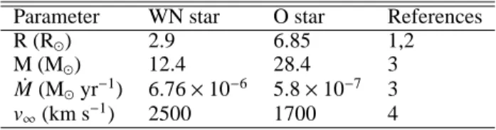
Table 1. V444 Cyg System Parameters

Parameter WN star O star References

R (R⊙) 2.9 6.85 1,2

M (M⊙) 12.4 28.4 3

˙

M (M⊙yr−1) 6.76 × 10−6 5.8 × 10−7 3

v∞(km s−1) 2500 1700 4

Notes. References: 1 (Corcoran et al. 1996); 2 (Eri¸s & Ekmekçi 2011);

3 (Hirv et al. 2006); 4 (Stevens et al. 1992)

Cyg has been insufficient to place reliable constraints on these processes until now.

Bhatt et al. (2010) and Fauchez et al. (2011) have both an-alyzed the 2004 XMM-Newton observations of V444 Cyg, which covered only half of the system’s cycle. Analysis by Fauchez et al. (2011) suggested some unexpected results con-cerning the wind collision region. These authors found that the hard X-ray emitting region may be positioned close to the WN star, suggesting that strong RIB processes may occur within the system (Owocki & Gayley 1995; Stevens & Pollock 1994). We obtained new XMM-Newton observations to complete the X-ray light curve and confirm this interpretation. In addition, Coriolis distortion due to the orbital motion of the stars may affect the shape and orientation of the wind-wind interaction region. Our new observations test this prediction by investigating whether the two halves of the light curve mirror each other. Any asym-metries in the light curve can be used to construct a quantitative model of the wind collision region and provide important new information about its structure.

Optical spectropolarimetric observations can place addi-tional constraints on the geometry of circumstellar material within the system. Light scattering from free electrons in the ionized circumstellar material is responsible for the phase-dependent polarization observed in V444 Cyg (Robert et al. 1989; St-Louis et al. 1993). Since electron scattering preserves geometric information about the scattering region, analyzing the polarization behavior of the system as a function of wavelength and orbital phase allows us to describe the scattering regions that produce the polarization in different spectral features. In the UBVRI bands, the observed phase-locked linear polariza-tion variapolariza-tions are dominated by the O star’s occultapolariza-tion of pho-tons originating from the WR star and scattering in a region of varying electron density (St-Louis et al. 1993). St-Louis et al. (1993) also found that the polarization behavior of the system near secondary eclipse deviates from the theoretical predictions of Brown et al. (1978), possibly due to the WR wind’s distortion from spherical symmetry as a result of the binary’s orbital mo-tion. Kurosawa et al. (2002) modeled the continuum polarization and found that they could reproduce the observations with the WR wind alone; the presence of the O-star wind and the wind-wind collision region do not affect the continuum polarization.

In this paper, we present the results of four new XMM-Newton observations, which we combine with six archival XMM-Newton observations to construct an X-ray light curve of the system with the best coverage to date. We supplement the XMM-Newton data with new observations from Swift that cover both eclipses. The optical and infrared primary (WN star in front of the O star) and secondary eclipses (O star in front of the WN star) are well covered with our combined data sets.

We also present new polarization curves of the V444 Cyg sys-tem in several strong optical emission lines, using data obtained with the University of Wisconsin’s Half-Wave Spectropolarime-ter (HPOL) at the Pine Bluff and RitSpectropolarime-ter Observatories. Our re-sulting multi-wavelength, multi-technique study provides new information about the structure of the winds (through spectropo-larimetry) and wind-wind interaction region (through X-rays), which we use to infer details about the 3D nature of the shock and wind structure. In Section 2 we describe our observations. Section 3 presents our observational results, including X-ray light curves, X-ray spectra, and line polarization variations. In this section we also discuss initial interpretations. We analyze our findings in Section 4 using simple modeling techniques and summarize our conclusions in Section 5.

2. Observations

This study uses data from several distinct data sets. Our first set of data consists of ten X-ray observations taken during two dif-ferent years with the XMM-Newton European Photon Imaging Cameras (EPIC); the second set is 40 ksec of observations of V444 Cyg taken over two weeks by Swift. The third data set con-sists of 14 observations taken with the University of Wisconsin’s Half-Wave Spectropolarimeter (HPOL) at the 0.9m telescope at Pine Bluff Observatory (PBO); and the last includes 6 observa-tions obtained with HPOL at the 1.0m telescope at the University of Toledo’s Ritter Observatory. We phased all observations using the ephemeris given by Eri¸s & Ekmekçi (2011)

T = HJD 2441164.311 + 4.212454E,

where E is the decimal number of orbits of the system since the primary eclipse, when the O star is eclipsed by the WN star, that occurred on HJD 2, 441, 164.311.

2.1. XMM-Newton

Our ten XMM-Newton observations were taken using the EPIC instrument in full frame mode with the medium filter. The first six of those observations are from 2004 while the last four were taken in 2012. The lengths of the observations vary; see Table 2 for their observation ID numbers, revolution numbers, start times, durations, and phase ranges. In total they cover approx-imately 65% of the orbit.

We reduced all of these observations using version 12.0.1 of the XMM-Newton SAS software. Because of the faintness of the source, pile up is not a problem; however, background flares were excised from several observations (see Table 2). Addition-ally, data from both MOS CCDs for observation 0206240401 (revolution number 0819) were not usable due to a strong flare affecting both MOS1 and MOS2 exposures. For each XMM-Newton observation, we extracted spectra for all EPIC cameras in a circular region with a 30" radius around the source such that oversampling is limited to a factor of five and the min-imum signal-to-noise ratio per bin is three. We extracted the background from a nearby area that was 35" in radius and de-void of X-ray sources. Additionally, we extracted light curves for these regions, correcting the data for parts of the point spread function not in the extraction region (using SAS task

epiclccorr) and correcting to equivalent on-axis count rates. We created light curves for each observation in the soft (0.4-2.0 keV), medium (2.0-5.0 keV), hard (5.0-8.0 keV), and total (0.4-10.0 keV) bands.

Table 2. XMM-Newton Observation Information for V444 Cyg

Obs. ID Rev. Start Time (HJD) Duration (s) Phase Rangea Flare?

0206240201 0814 2453144.997 11672 0.112-0.171 No 0206240301 0818 2453152.986 11672 0.011-0.070 No 0206240401b _{0819 2453154.986 10034 0.485-0.545 Yes} 0206240501 0823 2453162.969 11672 0.385-0.444 No 0206240701 0827 2453170.943 11672 0.284-0.343 Yes 0206240801 0895 2453306.476 19667 0.450-0.510 Yes 0692810401 2272 2456053.363 45272 0.505-0.683 No 0692810601 2275 2456059.025 18672 0.870-0.929 Yes 0692810501 2283 2456075.221 13672 0.727-0.787 Yes 0692810301 2292 2456093.118 50067 0.941-0.119 No

Notes.(a)_{Phases were calculated using the ephemeris from Eri¸s & Ekmekçi (2011).}(b)_{Data from MOS1 and MOS2 were lost for this observation}

due to a strong flare.

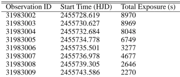
Table 3. Swift-XRT Observation Information for V444 Cyg

Observation ID Start Time (HJD) Total Exposure (s)

31983002 2455728.619 8970 31983003 2455730.627 8969 31983004 2455732.684 8048 31983005 2455734.778 6749 31983006 2455735.501 3277 31983007 2455736.978 4677 31983008 2455739.305 2646 31983009 2455743.586 2270 2.2. Swift

Swift observed V444 Cyg for 40 ks over the course of two weeks in 2011 with the XRT instrument (see Table 3). Because obser-vations were not continuous, we list only the start time and the total exposure for each observation ID. We processed the Swift data with the online tool at the UK Swift Science Data Center1_,

which produced a concatenated light curve with 100s bins, built for the soft (0.4-2.0 keV) and total (0.4-10.0 keV) bands. The small bins were then aggregated into 8 phase bins (0.00-0.5, 0.05-0.10, 0.40-0.45, 0.45-0.50, 0.50-0.55, 0.55-0.60, 0.90-0.95, and 0.95-1.00). Our observations have no pile up because count rates are low (between 0.01 and 0.04 cts s−1_).

2.3. HPOL

Our HPOL data can be divided into two subgroups. Taken be-tween 1989 October and 1994 December, the first 14 HPOL ob-servations used a Reticon dual photodiode array detector with a wavelength range of 3200-7600 Å and a resolution of 25 Å (see Wolff et al. 1996 for further instrument information). During this period HPOL was at the Pine Bluff Observatory (hereafter HPOL@PBO). The last six observations were con-ducted between 2012 May and 2012 December with the refur-bished HPOL at Ritter Observatory (hereafter HPOL@Ritter; see Davidson et al. 2014 for HPOL@Ritter instrument informa-tion). These four observations used a CCD-based system with a wavelength range of 3200 Å-10500 Å, and a spectral resolu-tion of 7.5 Å below 6000 Å and 10 Å above (Nordsieck & Harris 1996).

Table 4 lists the orbital phase along with the civil and he-liocentric Julian dates for the midpoint of each HPOL obser-vation. All of the HPOL@PBO observations covered the full

1 _{http://www.swift.ac.uk/user_objects/}

spectral range of the Reticon detector system. Only one of the HPOL@Ritter observations (2012 Oct 22) covered the full spec-tral range of the CCD detector system; the others used only the blue grating (3200 Å-6000 Å). Each HPOL observation typi-cally lasted between one and three hours (approximately 0.010 to 0.030 in phase). We reduced the HPOL data using the RE-DUCE software package which is specific to HPOL and de-scribed by Wolff et al. (1996). Astronomers at PBO and Rit-ter Observatory deRit-termine instrumental polarization for HPOL by periodically analyzing observations of unpolarized standard stars (Davidson et al. 2014). We removed this contribution from the data as part of the reduction process.

3. Results

3.1. XMM-Newton and Swift light curves

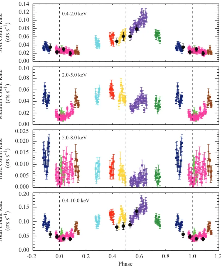
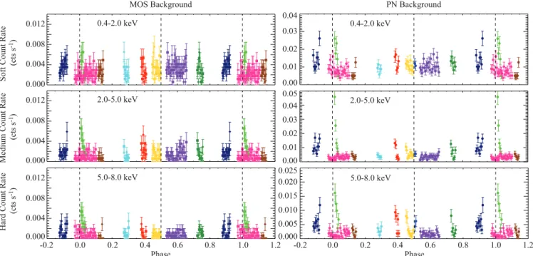
Our extracted light curves are displayed in Figures 1 (MOS1 and 2) and 2 (PN) with 2 ks binning in the following bands: soft (0.4-2.0 keV), medium (2.0-5.0 keV), hard (5.0-8.0 keV), and total (0.4-10.0 keV). We removed bins with a fractional expo-sure less than 0.5 due to low signal-to-noise ratios. In addition, the MOS data from observation 0206240401 (revolution 0819) are not shown in any band because they were lost due to a strong flaring event. The PN data have a higher count rate than the MOS data due to the higher sensitivity of the PN camera. We converted the count rates of our Swift observations into XMM-Newton equivalent rates using the WebPIMMS software pack-age and we overplot them in the soft and total bands (Figures 1 and 2). Although we have Swift data in the medium and hard bands, we do not plot those data here due to their large uncertain-ties. These represent the most complete X-ray light curves of the V444 Cyg system to date. Additionally, they are the first to cover both the ingress and egress of the system’s X-ray eclipses (phase 0.0 and 0.55), which allowed us to place important constraints on the size and location of the X-ray emitting region (Section 4). We describe the behaviors of each individual band below.

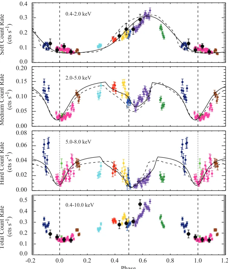
In the soft-band light curve, the minimum count rate occurs between phases 0.1 and 0.2, while the maximum occurs near phase 0.63 (top panels of Figures 1 and 2). The increase from minimum to maximum and the decrease from maximum to min-imum are smooth; however, the count rate increase to the max-imum occurs much more slowly than the subsequent decrease. This may indicate that the leading shock edge is brighter than the trailing edge. However, our data do no completely cover the decline.

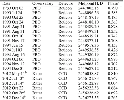
Table 4. HPOL Observation Information for V444 Cyg

Date Observatory Detector Midpoint HJD Phasea

1989 Oct 03 PBO Reticon 2447802.15 0.790

1990 Jul 24 PBO Reticon 2448096.26 0.583

1990 Oct 23 PBO Reticon 2448187.15 0.185

1990 Oct 24 PBO Reticon 2448188.10 0.363

1991 Aug 21 PBO Reticon 2448489.20 0.878

1991 Aug 31 PBO Reticon 2448499.31 0.252

1991 Oct 10 PBO Reticon 2448539.21 0.747

1991 Nov 17 PBO Reticon 2448577.11 0.708

1994 Jun 15 PBO Reticon 2449518.36 0.153

1994 Jul 03 PBO Reticon 2449536.35 0.426

1994 Aug 16 PBO Reticon 2449580.19 0.872

1994 Oct 06 PBO Reticon 2449631.23 0.978

1994 Nov 12 PBO Reticon 2449668.12 0.702

1994 Dec 01 PBO Reticon 2449687.12 0.212

2012 May 11b Ritter CCD 2456058.87 0.810 2012 Jul 13b Ritter CCD 2456121.83 0.767 2012 Jul 14b _{Ritter CCD 2456122.87 0.004} 2012 Oct 22 Ritter CCD 2456222.58 0.684 2012 Oct 26b _{Ritter CCD 2456226.69 0.692} 2012 Dec 14b _{Ritter CCD 2456275.55 0.265}

Notes.(a)_{Phases were calculated using the ephemeris in Eri¸s & Ekmekçi (2011).}(b)_{These observations used only the blue grating (3200 – 6000}

Å). All other HPOL observations are full spectrum for their respective detectors.

The medium-band and hard-band light curves (second and third panels of Figures 1 and 2) show eclipses with minima near phase 0.0 (primary eclipse) and 0.55 (secondary eclipse). Al-though the primary eclipse is symmetric in phase, the secondary eclipse is not; it starts at approximately phase 0.47 but ends at phase 0.63. Therefore, the system enters secondary eclipse more quickly than it recovers from it. Additionally, the count rate is higher just before secondary eclipse than just afterward.

Since the medium and hard X-rays likely come from higher temperature gas than soft X-rays and the eclipses of the gas oc-cur near the same phases as the optical eclipses, this behavior can be explained by physical occultation effects. That is, the eclipses in the medium and hard X-rays occur when the stars occult hot plasma in the wind-wind collision in and around the stagnation point, where the two winds collide head on. However, the sec-ondary eclipse is broader in phase than the O star (approximately 0.1) so either the hard X-ray emitting region is large and never fully eclipsed, which is consistent with the count rate never drop-ping to zero, or the O-star wind is also responsible for a portion of the eclipse. In the latter less likely case, the count rate may never drop to zero because photons at these energies are not as readily absorbed within winds (see Marchenko et al. 1997 and Kurosawa et al. 2001). The asymmetry in the eclipse near phase 0.55 can be explained if the hard X-ray emitting region does not lie on the line of centers connecting the two stars due to Coriolis distortion of the wind-wind interaction region (see Section 4.1 for the implications of this scenario). Additionally the broad and deep (but nonzero) primary eclipse suggests that the WN star ap-pears larger than what is suggested by visual and ultraviolet light curve analysis (Cherepashchuk et al. 1984; St-Louis et al. 1993). The dense wind of the WN star gives rise to a wind eclipse that is broader than the eclipse created by the stellar surface alone.

Figures 1 and 2 show that the Swift observations are con-sistent with the XMM-Newton data in the soft band. In the total band, the Swift data are consistent with the XMM-Newton rates within uncertainties, except near phase 0.6, where the XMM-Newton PN count rate is lower. The Swift data show less vari-ability than the XMM-Newton data due to their large phase bin-ning.

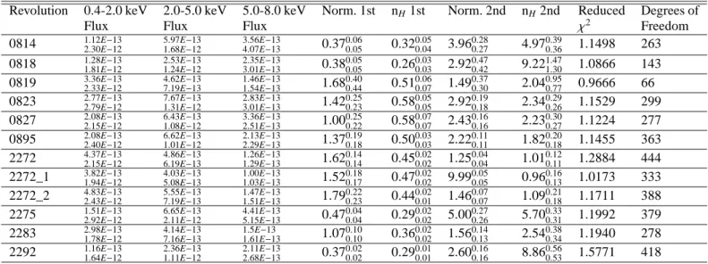
In the few places where the XMM-Newton observations over-lap in phase, they show good agreement and are clearly phase-locked, particularly in the soft band, even though the data sets were taken during different orbits of the system and were some-times separated by several years. This is particularly evident near phases 0.0 and 0.5, where observations from different orbits and years would be indistinguishable from each other without the color coding in Figures 1 and 2. However, in the medium and hard bands, observations near primary eclipse (0818 and 2292) are not always consistent with each other. There also appears to be a fair amount of stochastic variability in the light curves, possibly due to instabilities in the system’s stellar winds. For ex-ample, observations 2275 (dark blue in Figures 1 and 2), 0827 (light blue), and 0895 (yellow) exhibit apparently stochastic fluc-tuations in count rate around the global light curves. We find no correlation between these variations and the behavior of the background count rate (Figure 3), which suggests they are in-trinsic to the V444 Cyg system. However, these departures are similar in size to the uncertainties on the count rates, so their importance still remains unclear. Additional X-ray observations of V444 Cyg are needed to understand and determine the exact characteristics of this behavior. Next-generation X-ray observa-tories with much larger collecting areas will provide the preci-sion needed to investigate these stochastic variations and their relationship to massive star winds.

3.2. XMM-Newton spectra

We display all our extracted XMM-Newton spectra in Figure 4. The four observations (revolution numbers 0814, 0818, 2275 and

-0.2

0.0

0.2

0.4

0.6

0.8

1.0

1.2

Phase

T

ot

al

Count

Ra

te

(c

ts

s

-1

)

0.00

0.20

0.10

0.15

0.05

0.4-2.0 keV

2.0-5.0 keV

5.0-8.0 keV

0.4-10.0 keV

S

oft

Count

Ra

te

(c

ts

s

-1

)

0.00

0.14

0.02

0.04

0.06

0.08

0.10

0.12

0.00

0.02

0.04

0.06

0.08

0.10

M

edi

um

Count

Ra

te

(c

ts

s

-1

)

H

ard Count

Ra

te

(c

ts

s

-1

)

0.020

0.015

0.010

0.005

0.025

0.000

Fig. 1. X-ray count rates from the Swift (black crosses), XMM-Newton MOS1 (diamonds), and MOS2 (squares) observations discussed in

Sec-tion 3.2. Colors indicate data from different XMM-Newton observaSec-tions: revoluSec-tion number 0814=brown; 0818=green; 0819=blue; 0823=red; 0827=light blue; 0895=yellow; 2272=purple; 2275=dark blue; 2283=dark green; and 2292=pink. Swift data have been converted into an

XMM-Newton equivalent count rate using the WebPIMMS software package. From top: Count rate in the soft (0.4-2.0 keV), medium (2.0-5.0 keV), hard

(5.0-8.0 keV), and total (0.4-10.0 keV) bands versus phase. All data have been wrapped in phase so that more than one complete cycle is shown. The dotted vertical lines represent phases 0.0, 0.5, and 1.0.

-0.2

0.0

0.2

0.4

0.6

0.8

1.0

1.2

Phase

0.4-2.0 keV

2.0-5.0 keV

5.0-8.0 keV

0.4-10.0 keV

0.0

0.4

0.2

0.1

0.3

S

oft

Count

Ra

te

(c

ts

s

-1

)

0.00

0.20

0.10

0.05

0.15

M

edi

um

Count

Ra

te

(c

ts

s

-1

)

0.00

0.08

0.04

0.02

0.06

H

ard Count

Ra

te

(c

ts

s

-1

)

0.5

0.3

0.1

T

ot

al

Count

Ra

te

(c

ts

s

-1

)

0.4

0.2

0.0

Fig. 2. Same as Figure 1, but for the XMM-Newton PN camera. The solid lines in the top three panels represent the results of our occultation plus

WN-wind absorption model fits, while the dashed lines represent simulated light curves for the two-wind plus shock cone models (Section 4.1).

2292) around primary eclipse exhibit a double-humped spectral shape, while all other spectra are single-peaked. We have identi-fied many of the strong emission lines that appear in each obser-vation and display those identifications in the last panel.

To interpret these spectra, we fit the data with the XSPEC (v12.7.1) software package using the following two-component model (Arnaud 1996) with the same binning as the extracted

0.4-2.0 keV 2.0-5.0 keV 5.0-8.0 keV -0.2 0.0 0.2 0.4 0.6 0.8 1.0 1.2 Phase S oft Count Ra te (c ts s -1) M edi um Count Ra te (c ts s -1) H ard Count Ra te (c ts s -1) 0.000 0.004 0.012 0.008 0.000 0.004 0.012 0.008 0.000 0.004 0.012 0.008 MOS Background 0.4-2.0 keV 2.0-5.0 keV 5.0-8.0 keV 0.00 0.01 0.03 0.02 0.04 0.00 0.01 0.03 0.02 0.04 0.05 0.010 0.020 0.025 0.000 0.005 0.015 -0.2 0.0 0.2 0.4 0.6 0.8 1.0 1.2 Phase PN Background

Fig. 3. X-ray background count rates for the XMM-Newton MOS and PN cameras in the soft (0.4-2.0 keV), medium (2.0-5.0 keV), and hard

(5.0-8.0 keV) bands. The colors and vertical dashed lines are the same as those displayed in Figure 1.

spectra

wabs × (vphabs × vapec + vphabs × vapec),

where vapec is an emission spectrum from a diffuse and colli-sionally ionized gas, vphabs is a photoelectric absorption com-ponent, and wabs represents the interstellar medium absorp-tion component with a hydrogen column density fixed to nH = 0.32 × 1022 _cm−2 _{(Oskinova 2005). We refer to the abundance}

table of Anders & Grevesse (1989) for the other components. For each observation we fit the three EPIC spectra simulta-neously, except for observation 0206240401 (revolution 0819) where we only have PN data due to a strong flaring event. We performed the following careful step-by-step fitting procedure. First we allowed the temperatures, absorptions, and strengths (i.e. normalization factors within XSPEC) of the two com-ponents to vary freely, but we fixed the abundances to solar (Anders & Grevesse 1989). We found the temperatures of the two components to be constant with phase within their uncertain-ties: 0.6 keV for the first component and 2.0 keV for the second component. This is consistent with the analysis by Maeda et al. (1999) and expected for a colliding wind in a circular orbit where preshock speeds are constant. Therefore, we froze the tempera-tures of each observation at those values.

With these fixed temperatures we then allowed abundances to vary, linking the abundances of each individual element across the model components. This produced only one abundance per element during the fitting; in the following discussion we quote abundances in the XSPEC format (relative to hydrogen relative to solar). We allowed one abundance to vary at a time in the fol-lowing order: nitrogen (N), silicon (Si), sulfur (S), neon (Ne), magnesium (Mg), carbon (C), oxygen (O), and iron (Fe). While varying each individual abundance, we held all the others con-stant. We found the abundance of N to be about three times solar and constant with phase within uncertainties (i.e. we do not de-tect WN abundances at some phases, and O-star abundances at others). Therefore, we froze it at that value before moving on to the next element. Similarly, we found the Si, S, and Ne abun-dances for all of the spectra were solar within uncertainties, so

we froze them at 1.0. Magnesium was more abundant than solar; we froze it at 1.5. We found that C and O were comparable with a null value (likely due to high absorption providing little flux at C and O energies), so we set them to 0.0, while we found Fe to be just slightly lower than solar (0.8). These values are consistent with the results of Fauchez et al. (2011), but differ significantly from the abundances found by Bhatt et al. (2010), whose method of spectral modeling often resulted in unphysically large abun-dances. Figure 4 shows the resulting model fit for each of our EPIC observations.

After we completed the abundance fitting, the only free parameters remaining were the normalization and absorption columns (Table 5). The stellar separation in V444 Cyg does not change as a function of orbital phase because the orbit is circular. Therefore, the intrinsic emission from the system should be con-stant with phase, barring orientation effects such as occultation and absorption by wind material. We allowed the normalization and column density to vary in order to test for these effects. We display our fits’ resulting absorption columns and normalization parameters as functions of orbital phase in Figure 5.

The absorption of the 0.6 keV component stays nearly con-stant over the cycle (column 5 of Table 5; we note that the y axis in the bottom panel of Figure 5 is logarithmic). The lack of eclipse effects suggests that the soft emission arises in the outer regions of the stellar winds of the two stars, especially the WN wind. This behavior is reminiscent of that of WR 6, a single WN5 star (Oskinova et al. 2012). The soft X-ray emis-sion in WR 6 originates so far out that conventional wind shock models do not provide an adequate understanding of the mecha-nisms that generate it. In V444 Cyg, the 0.6 keV absorption is not uniformly constant, however; its slight increase between phases 0.22 and 0.6 is likely due to the O-star wind’s intrinsic emission becoming visible as the WN star and its wind rotate behind the O star. At these phases the WN wind is no longer absorbing the O-star emission along our line of sight. This increased absorp-tion comes from the fact that the soft intrinsic emission of the O star is emitted close to the photosphere, where absorption is

F e X X V F e X V II Ca X IX A r X V II S X V S i X III M g X I N e X 0814 0818 0819 0823 0827 0895 0.01 10-3 0.1 1.0 2272 2283 2275 N orm al iz ed Count s s-1 ke V -1 Energy (keV) Energy (keV) Energy (keV)

2292 si gn(da ta -m ode l) X de lt a c hi 2 0 5 -5 5 0 -5 0 -5 0 -5 5 -5 5 0 -5 5 0 5 0 -5 5 0 -5 5 0 -5 0.5 1.0 2.0 5.0 10.0 0.5 1.0 2.0 5.0 10.0 0.5 1.0 2.0 5.0 10.0 0.01 10-3 0.1 1.0 N orm al iz ed Count s s-1 ke V -1 si gn(da ta -m ode l) X de lt a c hi 2 0.01 10-3 0.1 1.0 N orm al iz ed Count s s-1 ke V -1 si gn(da ta -m ode l) X de lt a c hi 2 -5 5 0 Energy (keV) 0.5 1.0 2.0 5.0 10.0 0.01 0.1 1.0 N orm al iz ed Count s s-1 ke V -1 si gn(da ta -m ode l) X de lt a c hi 2 10-3

Fig. 4. XMM-Newton EPIC spectra. Green (PN), red (MOS2), and black (MOS1) points represent observed data from the different detectors within

the EPIC instrument. The solid lines in the same colors represent the XSPEC model fits discussed in Section 3.1. Spectra are indicated by their revolution number and arranged in phase order increasing from left to right across each row. Emission lines are identified in spectrum 2292.

larger compared to WN stars where this emission occurs farther from the star.

As expected, the absorption of the hotter component (2 keV) which arises from the wind-wind collision, is strongest when the WN star and its dense wind are in front of the wind collision region (phase 0.0). Similarly, the absorption of this component is weakest when the X-ray source is seen through the more ten-uous O-star wind, between phases 0.25 and 0.75. The length of this phase interval (half the orbital period) suggests that the bow

shock separating the O-star wind from the WN wind has a very large opening angle. We discuss this important result further in Section 4.

The absorption behavior of the spectral fits can be correlated with features in the soft X-ray light curve (Figures 1, 2, and 5, and Section 3.1). The phases when the WN star and its wind are in front (near primary eclipse) are the phases with the strongest absorption; they are also the phases at which the soft count rate is the lowest. More of the soft X-rays can escape the system

-0.2 0.0 0.2 0.4 0.6 0.8 1.0 1.2 Phase N orm al iz at ion (10 -3cm -5) 0 1 2 3 4 5 nH (10 22 cm -2) 0.1 10 1.0 0.6 keV Component 2.0 keV Component E m is si on M ea sure (10 41 c m -3) 0 2 4 6 8

Fig. 5. Normalization (top) and absorption column density (nH; bottom;

y axis is log scale) parameters from our spectral fitting of the

XMM-Newton observations as functions of phase. Circles (0.6 keV

compo-nent) and filled squares (2.0 keV compocompo-nent) represent the two different model components. In the case of observation 2272, we split the obser-vation at phase 0.624 as well as fitting the whole obserobser-vation (Section 3.1). Diamonds (open=0.6 keV, closed=2.0 keV) represent the two data sets derived from this split. Points are plotted in phase at the midpoint of each observation. Dotted vertical lines represent phases 0.0, 0.5, and 1.0. All data have been wrapped in phase so that more than one com-plete cycle is shown.

when the O star and its wind are in front because of that wind’s lower absorption. The spectral fits show that the absorption of the 0.6 keV component remains relatively constant between phases 0.25 and 0.75, despite the large variation in the soft count rate, whereas the 2 keV absorption component is highest when the WN star is in front. This can be understood by considering the emission is arising from the O-star wind. When the WN star is in front, the intrinsic X-ray emission from the O-star wind is absorbed by the WN wind, but when the O star is in front its intrinsic emission becomes visible. This explains the increase in the normalization of the 0.6 keV component in the 0.25 to 0.75 phase interval (Figure 5) and the increase in the soft-band count rate (Figures 1 and 2). Moreover, we attribute the asymmetry of the soft light curve to distortion from Coriolis deflection of the shock cone. In this senario, the distortion happens in such a way as to shift its maximum visibility toward later phases (i.e. the peak is near phase 0.63 instead of centered around phase 0.5). We discuss the interplay between the emission and absorption behavior of the system further in Section 4.1.

In addition to the above spectral fitting, we divided obser-vation 0692810401 (2272) into two separate spectra due to the large change in count rate over the course of the observation (see Figures 1 and 2). The observation was divided at phase 0.624 (2272_1 before, 2272_2 after) which is the approximate peak phase of the 0.4-2.0 keV light curve (Section 3.2).We per-formed spectral fitting on the two resulting spectra. We started our fitting process on the subdivided data with the best fit from the total observation (2272), keeping the same temperatures and abundances that were found to be constant on a global level (see previous discussion). The only free parameters were the normal-ization and absorption columns (Table 5 and Figure 5), which we found agreed with the total 2272 observation and the overall normalization and column density trends.

4000 5000 6000 7000 Wavelength (Å) P os it ion A ngl e 100 150 200 250 % P ol ari za ti on 0.0 0.5 1.0 1.5 2.0 H e II N IV H e I H α H e I H e II N V H e II + H β H e I N V H e II 0.0 0.5 1.0 1.5 Re la ti ve F lux (10 -1 1 e rg -1cm -1 s -1Å -1)

Fig. 6. Error-weighted mean polarization spectrum for HPOL@PBO

observations between phases 0.6 and 0.75. From top: relative flux, per-cent polarization, and position angle (degrees) versus wavelength. Gray dashed lines indicate identified emission lines. The polarization and po-sition angle data have been binned to 25Å . Error bars shown are the average polarization and position angle errors for the spectrum.

3.3. Optical polarimetry

Electron scattering in the ionized WN wind of V444 Cyg causes the system’s observed polarization (Robert et al. 1989; St-Louis et al. 1993). Continuum polarization light curves show phase-dependent variations that cannot be completely described by the standard, sinusoidal, ‘BME’-type behavior expected from detached binary stars (Brown et al. 1978; St-Louis et al. 1993). Deviations from that behavior near secondary minimum, in-cluding an asymmetric eclipse, indicate that the geometry of the WN wind is aspherical, likely due to the orbital mo-tion of the system (St-Louis et al. 1993). The emission lines in V444 Cyg also posses both linear and circular tion; de la Chevrotière et al. (2014) analyzed circular polariza-tion measurements of the He II λ 4686 emission line and de-tected no magnetic field. These authors noted the presence of variable linear polarization in the line, but attributed it to bi-nary orbital effects. However, because emission line photons may scatter in different locations within the wind than contin-uum photons, detailed analyis of linear line polarization vari-ations can reveal new information about the wind structure in V444 Cyg. We took advantage of the spectropolarimetric nature of our HPOL data to investigate the polarization behavior of the strongest emission lines in the optical regime. Figure 6 shows a sample polarization spectrum produced by taking the error-weighted mean of the four HPOL@PBO observations between phases 0.6 and 0.75 (Table 4), and binning the resulting stacked spectrum to 25Å; we have labeled many of the major emission lines.

Our observations contain polarization due to scattering by interstellar dust as well as electron scattering within the V444

Table 5. Spectral Fit Information for V444 Cyg XMM-Newton Observations

Revolution 0.4-2.0 keV 2.0-5.0 keV 5.0-8.0 keV Norm. 1st nH1st Norm. 2nd nH2nd Reduced Degrees of

Flux Flux Flux χ2 Freedom

0814 1.12E−13 2.30E−12 5.97E−13 1.68E−12 3.56E−13 4.07E−13 0.37 0.06 0.05 0.32 0.05 0.04 3.96 0.28 0.27 4.97 0.39 0.36 1.1498 263

0818 1.28E−13_1.81E−12 2.53E−13_1.24E−12 2.35E−13_3.01E−13 0.380.05_0.05 0.260.03_0.03 2.920.47_0.42 9.221.47_1.30 1.0866 143 0819 3.36E−13_2.33E−12 4.62E−13_7.19E−13 1.46E−13_1.54E−13 1.680.40_0.44 0.510.06_0.07 1.490.37_0.30 2.040.95_0.77 0.9666 66 0823 2.77E−13 2.79E−12 7.67E−13 1.31E−12 2.83E−13 3.01E−13 1.42 0.25 0.23 0.58 0.05 0.05 2.92 0.19 0.18 2.34 0.29 0.26 1.1529 299 0827 2.08E−13 2.15E−12 6.43E−13 1.08E−12 3.36E−13 2.51E−13 1.00 0.25 0.22 0.58 0.07 0.07 2.43 0.16 0.16 2.23 0.30 0.27 1.1224 277 0895 2.08E−13 2.40E−12 6.62E−13 1.01E−12 2.13E−13 2.29E−13 1.37 0.19 0.18 0.50 0.03 0.03 2.22 0.11 0.11 1.82 0.20 0.18 1.1455 363 2272 4.37E−13 2.15E−12 4.86E−13 6.19E−13 1.26E−13 1.29E−13 1.62 0.14 0.14 0.45 0.02 0.02 1.25 0.04 0.04 1.01 0.12 0.11 1.2884 444 2272_1 3.82E−13 1.94E−12 4.03E−13 5.08E−13 1.00E−13 1.03E−13 1.52 0.18 0.17 0.47 0.02 0.02 9.99 0.05 0.05 0.96 0.16 0.13 1.0173 333 2272_2 4.83E−13 2.43E−12 5.55E−13 7.19E−13 1.47E−13 1.51E−13 1.79 0.22 0.23 0.44 0.02 0.01 1.46 0.07 0.07 1.09 0.21 0.18 1.1711 388 2275 1.51E−13 2.92E−12 6.65E−13 2.11E−12 4.41E−13 5.15E−13 0.47 0.04 0.04 0.29 0.02 0.02 5.00 0.27 0.26 5.70 0.33 0.31 1.1992 379 2283 2.98E−13 1.78E−12 4.14E−13 7.16E−13 1.5E−13 1.61E−13 1.07 0.10 0.10 0.36 0.02 0.02 1.56 0.14 0.13 2.54 0.38 0.34 1.1940 278

2292 1.16E−13_1.64E−12 2.36E−13_1.11E−12 2.11E−13_2.68E−13 0.370.02_0.02 0.290.01_0.01 2.600.16_0.16 8.860.56_0.53 1.5771 418

Notes. These values were calculated by spectral fitting with the XSPEC software package (Section 3.1). Fluxes (columns 2, 3 and 4), normalizations

(columns 4 and 6), and column densities (columns 5 and 7) are in units of erg cm−2_s−1_{, cm}−5_{, and 10}22_cm−2_{respectively. Absorbed (upper) and}

unabsorbed (lower) fluxes are given for each observation in the soft, medium, and hard bands for which light curves were created (Section 3.2). Normalizations and column densities have high and low error bars as indicated. In the case of revolution 2272, we split the observation at phase 0.624 and performed spectral fitting of the resulting spectra as well as the whole observation (Section 3.1). Observation 2272_1 represents the spectra derived from the data between the start of observation 2272 and phase 0.624, while 2272_2 is from phase 0.624 to the end of the observation. See Section 3.1 for abundances used for all fits.

Cyg system. In a line region, the polarization produced within the system may include separate components for continuum and line polarization if they are scattered in different regions of the winds. Therefore, the observed polarization at each wavelength within an emission line is a vector sum of the three effects

%qobs=

QcFc+ QLFL+ QISPFtot

Ftot

, (1)

where Qc, QL, and QISPrepresent the Q Stokes parameters

de-scribing the continuum, line, and interstellar polarization, re-spectively, while Fc and FL denote the flux in the continuum

and line with Ftot = Fc+ FL. Parallel versions of this equation

and those below also hold for the Stokes U parameter. We note that because these are vector equations, the sign of each Q (U) parameter may be either positive or negative.

We calculated the polarization in the HeII λ4686, Hα, and NIV λ7125 emission lines using the flux equivalent width (few) method described by Hoffman et al. (1998). This allows us to separate the polarization into its continuum and line components without making any assumptions about the system. With this method we estimate the continuum flux and polarized flux within the line regions and subtract these quantities from the numerator and denominator of Equation 1

%qfew =

QcFc+ QLFL+ QISPFtot−(QcFc+ QISPFc)

Ftot−Fc

. (2)

This leaves, for each wavelength in the line region, %qfew=

QLFL+ QISPFL

FL

= %qL+ %qISP. (3)

To obtain a total polarization value for the line, we sum both numerator and denominator of Equation 3 over all contribut-ing wavelengths, which we choose as described below. Be-cause the interstellar polarization varies slowly with wavelength

(Serkowski et al. 1975; Whittet et al. 1992), QISPis very close to

constant over the wavelength region of an emission line. Thus the total polarization within an emission line is given by

%qentire line= (QL,1FL,1+ QISPFL,1) + (QL,2FL,2+ QISPFL,2) + ... FL,1+ FL,2+ ... = QL,1FL,1+ QL,2FL,2+ ... FL,1+ FL,2+ ... +QISP(FL,1+ FL,2+ ...) FL,1+ FL,2+ ...

= %qline all+ %qISP.

(4) In our discussion below, we report our measurements of %qentire lineand %uentire line, each of which is a simple vector sum

of the interstellar polarization and polarization produced within the system. We have made no attempt to remove ISP effects from our line polarization data, so these data cannot be taken to repre-sent absolute line polarization values. However, the constant ISP contribution produces only a simple linear shift in the zero point of the polarization in Figures 8-11. Because we expect that any ISP contribution will not vary with time over the period of our observations, we can attribute any time variability in the results to changes in polarization arising within the V444 Cyg system.

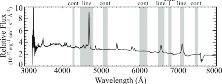
In order to estimate the continuum flux and polarization for the subtraction in Equation 2, we fit linear functions to the flux and polarization spectra between two wavelength regions on ei-ther side of the emission line (Figure 7). The choice of regions from which to estimate the continuum is important because the ISP has a shallow wavelength dependence, and because the in-clusion of a polarized line in a continuum region will skew the final polarization calculated for the line of interest. Therefore, we chose continuum regions near the emission line of interest that appear to have no emission or absorption features in our to-tal or polarized spectra. Figure 7 shows the continuum and line regions we used in our calculations.

3000 4000 5000 6000 7000 8000 Wavelength (Å) Re la ti ve F lux (10 -12 e rg -1 c m -1 s -1 Å -1) 0 4 6 8

line cont line line cont cont cont cont

2 10

Fig. 7. Relative total flux spectrum of V444 Cyg from 2012 Oct 22

using the HPOL@Ritter instrument setup. Gray areas mark the line and continuum regions we used to calculated the line polarization with the flux equivalent width method (Section 3.3) for each observation. We determined the underlying continuum for each line using the shaded continuum regions immediately to its red and blue sides.

In the case of the HeII λ4686 line we chose a line region that includes not only this line but also the NV λ4604 4620 doublet and the HeII λ4542 and HeI λ4471 lines, which are blended with each other in our spectra. This makes it more difficult to deter-mine which line is responsible for any phase-dependent polar-ization behavior; however, this ensures that we include all spec-tral regions which may be contributing to any variations. Simi-larly, the NIV λ7125 line has many absorption and emission lines around it, but we were able to define appropriate continuum re-gions and a line region that includes the line core without other stray lines. In the case of the Hα line we were able to define line and continuum regions more easily than for the other lines.

Photospheric absorption in the O star is an important source of line profile variations observed in total light (Marchenko et al. 1997; Flores et al. 2001). If we do not correct for this unpolar-ized absorption we risk removing too much continuum polariza-tion from our observapolariza-tions. We can correct for underlying ab-sorption features by treating them as part of the continuum in Equation 2; this reduces the value of Fcso as to produce a

spec-ified absorption equivalent width, as detailed by Hoffman et al. (1998). Marchenko et al. (1997) removed an absorption compo-nent from their V444 Cyg HeII λ4686 profile data by approx-imating the O-star absorption as a Gaussian line profile with a full width at half maximum (FWHM) of 6.0 Å and an EW of 1.0 Å. The same authors estimated an absorption profile for the HeI λ4471 line as a Gaussian with a FWHM of 6.0Å and an EW of 0.25 Å. While we do not know the EW of the NV dou-blet that is also blended with the HeII λ4686 line, we assumed an underlying unpolarized absorption component using a total EW of 2 Å . This value corrects for the absorption due to the He lines (1.25 Å total) while estimating a total absorption equivalent width of 0.75 Å for the N doublet. We found that the corrected line polarization values were not significantly different from the uncorrected values. Similarly, we found that for the Hα line, cor-rections on the order of half the total EW need to be made before the corrected values differ from the uncorrected by more than their uncertainties. This is significantly larger than the absorption EWs estimated for O stars (Kurucz et al. 1974, 2Å). Therefore, in the rest of this paper we present only the uncorrected data for all lines.

Table 6 tabulates the line polarization results we obtained us-ing the methods detailed above. To interpret these data, we need to understand how polarization is formed in the V444 Cyg sys-tem. Because both stars in the system are hot, we expect that electron scattering is the dominant polarizing mechanism for both line and continuum light. Zeeman splitting of spectral lines

due to magnetic fields can give rise to second-order effects in the Stokes Q and U parameters (Petit & Wade 2012). However, a recent study of V444 Cyg designed to detect Zeeman features in circular polarization (Stokes V) did not detect a magnetic field in the system (de la Chevrotière et al. 2014), so this effect is un-likely to cause the linear polarization we observe.

Even if electron scattering is the only polarizing mechanism at work, light in the emission lines may form, scatter, and/or be-come eclipsed in different regions than does light in the contin-uum. Analyzing these variations can help us further constrain the geometry of the emission and scattering regions in V444 Cyg. Although our data include a constant ISP contribution as dis-cussed above, their behavior with time provides important clues to the geometry of the line-scattering regions within V444 Cyg. Any variability in the line polarization indicates that the geom-etry of the system’s line-scattering region(s) is changing over time, due either to our changing perspective as the system ro-tates or to intrinsic changes in the distribution of scatters. If we observe no line polarization variability, we can assume that the geometry of the relevant line-scattering region remains constant over the time period of our observations.

Figures 8-11 show the phase-dependent polarization be-havior for the HeII λ4686, NIV λ7125, and Hα lines (Table 6). While emission lines in WR spectra are often unpolarized (Harries et al. 1998), our results show that this is not the case for V444 Cyg. If the lines were intrinsically unpolarized, then they would display a constant polarization due to the ISP contribu-tion, with no phase-dependent behavior. However, Figures 8-10 show that the polarization in the HeII λ4686 and NIV λ7125 lines varies with phase, implying that these lines contain polar-ization contributions arising from scattering within the system. By contrast, the Hα line polarization is consistent with zero in nearly all our observations. This could indicate either that it is intrinsically unpolarized (in which case the ISP contribution is necessarily small), or that its polarization is roughly constant with phase and nearly cancels out the ISP contribution. We dis-cuss this line behavior further at the end of this section.

Figures 8-11 also show that the polarization behavior of these three lines is not consistent with the broadband polarimetric be-havior found by St-Louis et al. (1993), which shows the stan-dard sinusoidal behavior expected from binary stars along with an asymmetric secondary eclipse effect due to distortion of the WN’s wind. This indicates that the continuum and line photons are polarized by different scattering regions within the system.

Since the HeII λ4686 emission line shows little phase de-pendence in the Stokes Q parameter, we calculated the error-weighted angle (−15◦_±5.8◦_{or equivalently 165}◦_±5.8◦_{) by which}

we would have to rotate our data to place all of the polarization variation in the resulting projected Stokes U parameter (Stokes U marks the 45◦_-135◦_{axis in unprojected Q-U space). This}

ro-tation causes the projected Stokes Q (which we depict in Figure 8 as a percentage, % qp) to average to zero. We do not interpret this rotation angle as an intrinsic axis within the system; rather, it is a tool to simplify the data for display and aid in our inter-pretation. In the rest of this section, we discuss the polarization behavior of the HeII λ4686 only line in terms of %up. We rotated the NIV λ7125 line by 10.4◦for the same reasons (uncertainty on the error-weighted mean is ±11◦_{), with the same caveat that}

this angle is not necessarily intrinsic to the system. In the case of the Hα line, both Stokes parameters remain zero within uncer-tainties for most of our observations. We therefore did not rotate these data.

After rotation, the values of % qp for the HeII λ4686 line remain positive for the first half of the light curve, but

scat-Table 6. HPOL Line Polarization Stokes Measurements

Hα HeII λ4686 NIV λ7125

Date Phase % q % u % Error % q % u % Error % q % u % Error

1989 Oct 03 0.790 -1.5110 -2.4579 0.9408 0.0654 -0.1774 0.2992 -0.6922 -0.6771 0.7119 1990 Jul 24 0.583 -0.0306 0.1236 0.9911 -1.0061 -1.4650 0.3212 -0.9406 0.0248 0.5935 1990 Oct 23 0.185 -1.4468 2.1103 0.8538 0.0068 0.4654 0.3375 0.2097 1.1375 0.5768 1990 Oct 24 0.363 -0.5154 -0.2944 0.7267 0.3231 -0.7084 0.2973 -0.7041 -0.8975 0.7494 1991 Aug 21 0.878 -1.0984 0.7828 1.0322 -0.6105 -0.4702 0.3845 0.9202 -0.0931 0.6354 1991 Aug 31 0.252 -0.0926 0.2813 0.9119 1.4296 -0.3627 0.4441 -0.4877 0.3206 0.7898 1991 Oct 10 0.747 -1.6390 -0.2771 0.6717 0.0549 -0.4787 0.3698 -0.0859 0.4593 0.5554 1991 Nov 17 0.708 0.2388 -1.6601 1.0027 -0.1982 -0.2855 0.4866 -0.6661 -0.0959 0.7179 1994 Jun 15 0.153 4.9108 0.9717 2.5127 0.9262 0.0591 0.7414 3.1580 2.5385 1.5831 1994 Jul 03 0.426 -0.6828 -0.6338 1.5643 1.1650 -1.5495 0.4584 -1.2326 -1.3260 1.2366 1994 Aug 16 0.872 1.0321 0.4674 1.2103 -0.2664 0.9080 0.5495 1.9333 0.5301 0.9724 1994 Oct 06 0.978 -0.8630 1.2595 1.3337 0.5983 -0.0933 0.5676 -0.3639 1.1728 0.9390 1994 Nov 21 0.702 1.3809 -1.5241 1.5728 0.3399 0.1109 0.7363 0.2433 -1.6902 1.4111 1994 Dec 01 0.212 -0.7050 0.2555 1.1458 0.7282 -1.0072 0.5716 -1.7630 1.8021 0.9190 2012 May 11 0.810 ... ... ... 1.5238 -0.7899 0.4783 ... ... ... 2012 Jul 13 0.766 ... ... ... 2.7477 -1.5460 0.5949 ... ... ... 2012 July 14 0.004 ... ... ... 1.0221 0.5791 0.8323 ... ... ... 2012 Oct 22 0.683 -0.1479 -0.5860 -0.0255 0.2886 0.3585 0.3585 0.3044 -0.1509 0.0972 2012 Oct 26 0.692 ... ... ... 0.5757 -0.7716 0.6236 ... ... ... 2012 Dec 14 0.265 ... ... ... -0.0076 -0.0467 0.3757 ... ... ... -0.2 0.0 0.2 0.4 0.6 0.8 1.0 1.2 Phase 0 -2 -1 1 2 3 4 % qp -2 0 -1 2 1 % up

Fig. 8. Data points represent the HeII λ4686 emission line polarization

from HPOL@PBO (open squares) and HPOL@Ritter (filled squares). From top: projected % qpStokes parameter and projected % upStokes parameter versus phase (see text; rotated by −15◦_{). The solid horizontal}

lines mark error-weighted mean values of % qpand % upfor the phase regions they span; 1σ uncertainties are shown in gray. Dotted vertical lines represent phases 0.0, 0.5, and 1.0. Dotted horizontal lines mark zero in % qpand % up.

ters around zero more evenly during the second half (Figure 8). In % up, the polarization shows variations of the same magni-tude (on the order of ±2%). Points between phases 0.6 and 1.0 have a larger scatter than the rest of the light curve, while ob-servations near secondary eclipse have a lower % up than the rest of the light curve. This lower pattern suggests that suggests V444 Cyg has a phase-locked polarization behavior. To quantify this behavior, we calculated the error-weighted mean % upfor the phase regions 0.30 to 0.75, and 0.75 to 1.30. Our choice of these two phase regions was guided by the differing behavior of the normalization and column densities seen in the X-ray spec-tra around secondary eclipse (Figure 5). The region around sec-ondary eclipse (phases 0.3 to 0.75) that has a low 2 keV

absorp--0.2 0.0 0.2 0.4 0.6 0.8 1.0 1.2 Phase 0 -2 4 2 % qp 6 -4 0 -2 4 2 % up 6 -4

Fig. 9. Same as Figure 8, but for the NIV λ7125 line. Stokes parameters

are rotated by 10.4◦_.

tion in X-rays also has a lower average % up (−0.703 ± 0.142) than the rest of the light curve (−0.193 ± 0.133), a discrep-ancy of nearly 2σ (compare Figures 5 and 8). The % qp aver-ages for those same phase intervals overlap within uncertainties (0.056 ± 0.142 for phases 0.30-0.75; 0.320 ± 0.133 for phases 0.75 to 1.30).

The NIV λ7125 line behaves similarly to the HeII λ4686 line (Figure 9); the % upvalues for this line are predominantly neg-ative around secondary eclipse (phases 0.3-0.75) where the X-rays have a low 2 keV component absorption feature (Figure 5) and are positive or zero at other phases. However, the % qp val-ues are negative in the 0.3 to 0.6 phase range, but scatter equally about zero at other phases. A similar analysis shows the error-weighted mean % up for observations between 0.3 and 0.75 in phase is significantly lower (−0.139 ± 0.085) than the rest of the cycle (0.579 ± 0.279), while the average % qp values for these two regions overlap (0.228 ± 0.085 for phases 0.30-0.75; 0.110 ± 0.279 for phases 0.75 to 1.30).

-0.2 0.0 0.2 0.4 0.6 0.8 1.0 1.2 Phase 0 -2 -1 1 2 3 % qp 0 -2 -1 1 2 3 % up

Fig. 10. Unrotated Stokes parameters for the HeII λ4686 (red dotted)

and NIV λ7125 (black solid) line data, binned to 0.1 in phase.

To directly compare the behavior of the two lines, we smoothed our polarization data by calculating the error-weighted mean unrotated %q and %u for bins of width 0.1 in phase; when we overplotted the smoothed curves (Figure 10), we found that these two lines show similar phase-dependent behavior. The %u values are more positive near phase 0.0 and first quadrature (phase 0.25) than around phase 0.5 while after secondary eclipse they gradually trend toward more positive values. In contrast, %q remains relatively flat during the first half of the orbit, while the variations in the second half are of a more stochastic nature.

We interpret these line polarization results as follows. Within the V444 Cyg system, the NIV emission should arise within the wind of the WN star, and the HeII is largely in a shell of material around the WN star (see Figure 8 in Marchenko et al. 1997). If these lines arose in the shells of HeII λ4686 and NIV

λ7125 around the WN star and scatter in the spherically symmet-ric WN wind, then we would measure no net polarization. The fact that we measure a phase-dependent polarization behavior in both lines suggests that the wind must be aspherical in some way. The WN wind is much more dense than the O-star wind (Stevens et al. 1992; Hirv et al. 2006), so one simple way to vi-sualize this asymmetry is to posit that the O-star wind carves out a less dense cavity within the WN wind. Kurosawa et al. (2002) used such a sphere plus cavity model to reproduce the observed continuum polarization variations in V444 Cyg. The emission line polarization should also contain signatures of this aspheric-ity, but these signatures will differ from those seen in the con-tinuum polarization because the line photons originate from the WN wind instead of form the stellar photospheres and may scat-ter in different locations within the wind.

For a sphere plus cavity model better suited to interpret our line polarization results, we turned to Kasen et al. (2004), who investigated the polarization behavior of a hole in the ejecta of a Type Ia supernova due to its unexploded companion star. While the density profiles in this scenario are different than those of the winds in V444 Cyg, this model is highly relevant to our case for several reasons. First, the ejecta hole produces a cone-shaped cavity resembling the shock-wind structure within V444 Cyg. Second, in the Kasen et al model, the density of material within the hole is 0.05 times that of the ejecta, which is analogous to the less dense O-star wind filling the cavity within the denser WN wind. (We note that the wind density ratio in V444 Cyg is difficult to calculate because it depends on the wind veloci-ties, which are in turn affected by the radiative forces discussed in Section 4.1). Third and most importantly, Kasen et al. (2004)

-0.2 0.0 0.2 0.4 0.6 0.8 1.0 1.2 Phase -4 0 -2 4 2 % u 0 -2 4 2 % q 6 -4 6

Fig. 11. Same as Figure 8, but for the Hα line. Stokes parameters are

unrotated.

considered a distributed emission source, with photon packets arising from throughout their model atmosphere to simulate the energy deposition from decaying56Ni and56Co into the super-nova ejecta. This distributed emission is also a good representa-tion of the line-emitting shells surrounding the WN star in V444 Cyg (Marchenko et al. 1997).

Kasen et al. (2004) oriented their models such that all the polarization variations occurred in one Stokes parameter. They found that for viewing angles near the axis of the hole, the polar-ization is negative, but it becomes more positive as the viewing angle moves away from the hole. Because we rotated our line data (Figures 8 and 9) such that most of the polarization varia-tion occurred in % up, we can draw an analogy between these variations and those predicted by the ejecta-hole model. Using this analogy, we can attribute the change in polarization behav-ior of our HeII λ4686 and NIV λ7125 lines to a ‘hole’ created by the shock cone (which we detect in our X-ray data) in the otherwise spherical shells around the WN star. As our viewing angle changes with phase, the changing geometry of the incom-plete shells causes the variations in polarization we observe. In this picture, the ‘hole’ is open to our light of sight at phases near secondary eclipse. The angle by which we rotated each line’s data thus corresponds to the geometrical offset between the ori-entation of the shells in V444 Cyg and the oriori-entation of the Kasen et al. (2004) model. These angels are similar for the two lines, but not the same; in addition, the lines show different polar-ization behavior with phase (Figure 10). If the ejecta-hole model is a good approximation of the winds in V444 Cyg, these dis-crepancies may simply indicate that the shock is a more complex structure than a cone and that the shells of material where lines form are misaligned.

Unsurprisingly, our data do not exactly reproduce the trends in polarization with viewing angle (phase) predicted by Kasen et al. (2004). One important difference between the case of V444 Cyg and the ejecta-hole scenario is the size of the open-ing angle of the shock hole. Our shock likely has a very large opening angle (see Sections 3.1 and 4.2), which means our view-ing angle always remains closer to the cavity than in Kasen’s models. We also have a shock structure with the same geometric shape as the hole, which makes it difficult to distinguish between light scattered in the wind and light scattered in the shock. In ad-dition, although we rotated our data in an attempt to confine the phase-locked polarization to the U Stokes parameter, both emis-sion lines still display relatively large changes in % qp(Figures 8 and 9). In the context of the cavity model, this might indicate

that at phases when we do not see the shock and the hole, the WN wind appears elongated rather than spherically shaped.

In contrast to the HeII λ4686 and NIV λ7125 lines, the Hα emission in V444 Cyg likely comes from cooler regions around the system. Figure 11 shows that both Stokes parameters in the Hα line are zero within uncertainties in the majority of our obser-vations. This implies that the polarization in this line is constant with phase, although it may not have an intrinsic value of zero because we have not removed the ISP contribution. A constant polarization indicates that the scattering region for the Hα line is far enough from the stars that their orbital motion not affect its geometry. The deviations from zero measured polarization do not appear to have a phase-dependent behavior, which suggests that clumping of material within the cooler regions of the sys-tem may be responsible for the variability (Li et al. 2009). Such clumps are likely transient and unconnected to the orbital period of the system; thus, any polarization produced by scattering in this clumpy wind should be stochastic as suggested in Figure 11. The emission lines in V444 Cyg are polarized at least in part by scattering within the system; they show polarization vari-ations different from those of the continuum because the line and continuum photons originate from different regions. Despite these distinctions, our spectropolarimetric results support the cavity model developed by Kurosawa et al. (2002) to describe the wind structure in the system. The phase correlation we ob-serve between the decrease in 2 keV X-ray column density (Sec-tion 3.2) and the decrease in emission line polariza(Sec-tion provides the first concrete evidence tying polarimetric variations to the presence of a low-density cavity in the WN wind.

4. Discussion

The behavior we see in both the X-rays and spectropolarimetry can be explained by a combination of three effects: 1) simple geometric eclipses; 2) distortion of the stellar winds due to the orbital motion of the stars; and 3) the presence of a cavity in the WN wind produced by its collision with the wind of the O star. Our X-ray light curves and spectra provide direct constraints on the geometry of the interacting winds in the system. Below we discuss simple models of these data that allow us to draw some basic conclusions about the V444 Cyg system. We adopt the sys-tem parameters in Table 1 and a separation of a = 35.97 R⊙

(Eri¸s & Ekmekçi 2011). We do not calculate formal uncertain-ties on our models’ outputs because of their simplicity; it is clear a more sophisticated treatment of the system is needed, which we plan to address in a future paper.

4.1. Modeling the X-ray Light Curves

To further interpret the phase variation of the XMM data in the soft, medium, and hard bands, we modeled the colliding-wind X-rays of V444 Cyg with an analytic occultation plus WN-wind– absorption model with a geometry shown in Figure 12. We define the x-axis as the line of centers between the stars; our modeled X-ray emission then originates from a circle (yellow in Figure 12) in the yz-plane, where y is the direction of orbital motion (+y for the O star) and z is the orbital axis. The circle of ra-dius rcis located a distance xc(blue) from the WN star and is offset a distance ycalong purple line in Figure 12 from the line between the stars. Since the system’s circular orbit implies con-stant emission, all phase variation in X-rays is due to changes in the absorption and occultation of the X-ray emitting region. Our model calculates 64 mass column densities mc(black) along

rays from points evenly distributed around the circle to the ob-server, whose perspective is rotated around the system (in the xy-plane) at inclination i = 78.3◦(from the +z-axis) to determine the phase dependence of mc. When emission locations are occulted by the O star (red) or WN star (cyan), we set the column density to infinity, while the mcof unocculted locations are determined by setting the entire circumstellar environment to be WN wind material (gray). Therefore our model overestimates the circum-stellar absorption in regions that would be occupied by the less dense O-star wind, but also underestimates the absorption col-umn for regions where the line of sight passes through shocked material.

We compute the density ρ of the WN wind from a spherically symmetric, constant-mass-loss, β = 1 velocity-law wind with pa-rameters from Table 1; the column depth integral mc =

R ρdz′

(where z′is the direction of the observer) is thus solved in closed form. We then compute optical depths to each point on the circle using a band-appropriate opacity κ(E) (i.e. energy E is within the waveband), such that the relative X-ray flux is

LX(φ, E) =

64

X

i=1

w(i) exp(−mc,i(φ)κ(E)), (5) where φ is phase and w(i) is the emission weighting of each point on the circle (see below). We choose κ(E) to be consistent with opacities from a WN windtabs model (Leutenegger et al. 2010). Since this model only produces relative X-ray fluxes, we use a linear and constant normalization term to convert equa-tion 5 to XMM-Newton PN cts s−1 _{for model-to-data}

compar-isons (Figure 2).

The emission from all points around the circle is not neces-sarily equal; a larger portion of the wind flows perpendicularly to the shock front on the prograde side than on the retrograde side, so the prograde side should emit more strongly in X-rays (see e.g. Pittard 2009). In V444 Cyg the stronger WN wind leads to the shock front wrapping around the O star, so our model sets the emission weighting of the O-star’s prograde edge of the circle to wprotimes the emission of the retrograde edge wret= 1. For

inter-mediate points i, we set the weight w(i) to w(i) = f (i)(wpro−1)+1,

where f (i) = (y(i) - yc+rc)/(2rc) is the fractional distance along the horizontal line through the emitting circle’s center (y direc-tion, purple dashed line in figure 12) from the retrograde edge (yc−rc) to the prograde edge (yc+ rc).

Our optimal light-curve models are displayed as solid lines in Figure 2 for the soft (top), medium (second panel), and hard (third panel) bands. The parameters for those models are listed in Table 7. Each observed light curve varies more significantly than can be explained by our occultation plus WN-wind–absorption model, so instead of performing formal statistics to determine a best fit to all data points, we obtain an optimal fit for each waveband by attempting to match the main features of each light curve. The soft model light curve reproduces the sought-after minimum around phase 0.05 and peak just after phase 0.6, but our model peak is not as sharp as that of the observed light curve. However, if we fit the more narrow shape from phase 0.5–0.7, we do not reproduce the gradual change in X-rays over the remain-ing phases. This might indicate that a two-component model would be more appropriate; in this case one circle of emission would reproduce the narrow shape between phases 0.5 and 0.7 after the O star passes in front of the WN star, and the other would produce the more gradual trend seen throughout the orbit. Since there is no a priori method for combining relative fluxes between two light curves, we do not consider a two-component model here. Another explanation for the observed peak shape