VIP: Vortex Image Processing Package for High-contrast Direct Imaging
Carlos Alberto Gomez Gonzalez1, Olivier Wertz1, Olivier Absil1,10, Valentin Christiaens1,11,12, Denis Defrère1, Dimitri Mawet2,13, Julien Milli3, Pierre-Antoine Absil4, Marc Van Droogenbroeck5,
Faustine Cantalloube6,14, Philip M. Hinz7, Andrew J. Skemer8, Mikael Karlsson9, and Jean Surdej1,15
1
Space Sciences, Technologies & Astrophysics Research(STAR) Institute, Université de Liège, Allée du Six Août 19c, B-4000 Liège, Belgium
2
Department of Astronomy, California Institute of Technology, Pasadena, CA 91125, USA
3European Southern Observatory, Santiago, Chile 4
Department of Mathematical Engineering, Université catholique de Louvain, B-1348 Louvain-la-Neuve, Belgium
5
Institut Montefiore, Université de Liège, B-4000 Liège, Belgium
6
CNRS, IPAG, F-38000 Grenoble, France
7
Steward Observatory, Department of Astronomy, University of Arizona, 933 N. Cherry Avenue, Tucson, AZ 85721, USA
8
University of California, Santa Cruz, 1156 High Street,Santa Cruz, CA 95064, USA
9
Department of Engineering Sciences, Ångström Laboratory, Uppsala University, Box 534, SE-751 21 Uppsala, Sweden Received 2016 June 23; revised 2017 May 9; accepted 2017 May 15; published 2017 June 13
Abstract
We present the Vortex Image Processing (VIP) library, a python package dedicated to astronomical high-contrast imaging. Our package relies on the extensive python stack of scientific libraries and aims to provide a flexible framework for high-contrast data and image processing. In this paper, we describe the capabilities of VIP related to processing image sequences acquired using the angular differential imaging(ADI) observing technique. VIPimplements functionalities for building high-contrast data processing pipelines, encompassing pre- and post-processing algorithms, potential sourceposition and flux estimation, and sensitivity curvegeneration. Among the reference point-spreadfunction subtraction techniques for ADI post-processing, VIP includes several flavors of principal component analysis (PCA) based algorithms, such as annular PCA and incremental PCA algorithms capable of processing big datacubes(of several gigabytes) on a computer with limited memory. Also, we present a novel ADI algorithm based on non-negative matrix factorization, which comes from the same family of low-rank matrix approximations as PCA and provides fairly similar results. We showcase the ADI capabilities of the VIP library using a deep sequence on HR 8799 taken with the LBTI/LMIRCam and its recently commissioned L-band vortex coronagraph. Using VIP, we investigated the presence of additional companions around HR 8799 and did notfind any significant additional point source beyond the four known planets. VIP is available athttp://github. com/vortex-exoplanet/VIP and is accompanied with Jupyter notebook tutorials illustrating the main functionalities of the library.
Key words: methods: data analysis– planetary systems – planets and satellites: detection – techniques: high angular resolution– techniques: image processing
1. Introduction
The field of exoplanets is presently one of the most active areas of modern astrophysics. In only two decades of exoplanetary science, we count more than 3000 confirmed discoveries, most of which have been made possible thanks to indirect methods (Pepe et al. 2014). Only a few tens of
exoplanets could be directly resolved through high-contrast imaging. The task of finding exoplanets around their host starswith direct observations is very challenging and has been enabled in the last decade thanks to technological advances in ground-based NIR instruments, adaptive optics, and corona-graphy. Direct observations of exoplanets provide a powerful complement to indirect detection techniques and enable the exploration, thanks to its high sensitivity to wide orbits, of different regions of the parameter space. Direct imaging also
allows us to put important constraints in planet formation models and planetary systems dynamics and, since we obtain the photons from the planets themselves, we can proceed with further photometric and spectroscopic characterization (Oppen-heimer & Hinkley2009; De Rosa et al.2016).
High-contrast direct imaging from the ground presents three main challenges: the huge difference in contrast between the host star and its potential companions (typically ranging from 10−3to 10−10), the small angular separation between them, and the image degradation caused by the Earth’s turbulent atmosphere and optical imperfections of the telescope and instruments. These challenges are addressed with a combined effort of coronagraphy, optimized wavefront control, dedicated observing techniques, and image post-processing(Guyon2005; Mawet et al.2012).
Among the observing strategies, angular differential imaging (ADI, Marois et al.2006) is the most commonly used high-contrast
imaging technique, in spite of its limitations, and is the focus of this paper. ADI can be paired with several post-processing algorithms, such as the least-squares based LOCI (locally optimized combination of images, Lafrenière et al. 2007), the
maximum likelihood based ANDROMEDA(Mugnier et al.2009; Cantalloube et al.2015), and the family of principal component
© 2017. The American Astronomical Society. All rights reserved.
10
F.R.S.-FNRS Research Associate.
11
Departamento de Astronomía, Universidad de Chile, Santiago, Chile.
12
Millennium Nucleus“Protoplanetary Disks,” Chile.
13
Jet Propulsion Laboratory, 4800 Oak Grove Drive, Pasadena CA 91109, USA.
14
Office National d’Etudes et de Recherches Aérospatiales (ONERA), Optics Department, BP 72, 92322 Châtillon, France.
15
analysis (PCA) based algorithms (Amara & Quanz 2012; Soummer et al.2012). Recent algorithms such as LLSG (Gomez
Gonzalez et al. 2016a) aim to decompose the images into
low-rank, sparse, and Gaussian-noise terms in order to separate the companion signal from the star point-spread function (PSF) and specklefield. A common step in any of these approaches is the use of a model PSF. Algorithms of different complexities are used to build these optimal reference PSFs and enhance the detectability of potential planets and disks in the presence of speckle noise. From now on, and throughout this paper, we call the reference PSF the algorithmically built image that we use with differential imaging techniques for subtracting the scattered starlight and speckle noise patternand enhancing the signal of disks and exoplanets.
This paper presents a python library for image processing of high-contrast astronomical data: the Vortex Image Proces-sing(VIP, Gomez Gonzalez et al.2015,2016b) package. VIP
provides a wide collection of pre- and post-processing algorithms and currently supports three high-contrast imaging observing techniques: angular, reference-star, and multi-spectral differential imaging. The code encompasses not only well-tested and efficient implementations of known algorithms but also state-of-the-art new approaches to high-contrast imaging tasks. Our library has been designed as an instru-ment-agnostic toolbox featuring a flexible framework where functionalities can be plugged in according to the needs of each particular data set or pipeline. This is accomplished while keeping VIP easytouse and welldocumented. Finally, our package is released as opensource hoping that it will be useful to the whole high-contrast imaging community.
This paper is organized as follows. Section2gives a general overview of the design and structure of the VIP. In Section3,we briefly describe the pre-processing and cosmetic functionalities implemented in VIP. Section 4 presentsthe details of reference PSF subtraction for ADI data, exploring the available post-processing algorithmic approaches in VIP. Section 5describes the photometric and astrometric extraction technique implemented in our package. Section6describes the sensitivity limitestimation, and finally Section 7 showcases VIPusing on-sky data.
2. Package Overview
The design and development of VIP follow modern practices for scientific software development such as code modularity, the active use of a version control system (git) and extensive documentation(Wilson et al.2014). The code is
being developed in python, and relies on its vast ecosystem of scientific open-source libraries/packages including numpy (van der Walt et al. 2011), scipy (Jones et al. 2001),
matplotlib(Hunter2007), astropy (Astropy
Collabora-tion et al. 2013), scikit-learn (Pedregosa et al. 2011),
pandas (McKinney 2010),and scikit-image (van der
Walt et al. 2014). For low-level image processing operations,
VIPcan optionally use, through its python bindings, OpenCV (Bradski 2000), a fast and robust C/C++ library
for computer vision and image processing. The latest development version of VIP is available on GitHub,16which is also the platform where users and/or collaborators can report bugs and make change requests. Every function and class in VIP has its own internal documentation attached describing the aim, arguments (inputs), and outputs. The internal
documentation is part of the VIP’s web documentation,17 which also provides help in installation and troubleshooting. A tutorial dedicated to ADI, in the form of a Jupyter notebook, is shipped in the main repository of VIP.
The structure of VIP, shown in Table 1, is modular and allows easy extension and re-utilization of functionalities. The code is organized, as any other python library, in sub-packages (directories) encapsulating modules (python files), which in turn contain the functions and classes. It is important noting that VIP is not a pipeline per se but a library, inspired in well established projects such as astropy or scikit-learn, and does not provide a predefined linear workflow. Instead, the user must choose which procedures to use and in which order. The results of VIP’s calculations are kept in memory or displayed, e.g., in plots orfigures, andlater on can be saved to disk in the form of fits files. In the following paragraphs, we describe briefly the most relevant functional-ities of each subpackage of VIP.
Thefits subpackage includesfunctions for handling files in the FITS format, through Astropy functionalities. It also includes a python class, which allows controlling SAO-Image DS9windows (based on the interface to SAOImage DS9 through XPA from the RO python package) and displaying numpy arrays. Thanks to these functions, VIP can be fed with any FITS file containing a high-contrast imaging datacube.
The subpackage phot includes functionalities such as signal-to-noise ratio (S/N) estimation, S/N mapgeneration, automatic detection of point-like sources, fake companion injection in ADI cubes, and sensitivity limitcomputation. For aplanet S/N calculation, we implement the small sample statistics approach proposed by Mawet et al. (2014), which
uses a two-sample t-test with statistics computed over resolution elements (circular apertures of l D diameter) instead of considering the pixels as statistically independent (Mawet et al. 2014; Gomez Gonzalez et al. 2016a). The
subpackage stats contains functions for computing statistics from regions of frames or cubes, sigma filtering of pixels in frames, and for computing distance and correlation measures
Table 1 VIPSubpackages Subpackage General description
conf Timing, configuration, and internal utilities exlib Code borrowed from external sources fits Fits input/output functionality
llsg Local low-rank+ sparse + Gaussian-noise decomposition for ADI data
madi Standard ADI recipe(median PSF reference)
negfc Negative fake companion technique forflux and position estimation
nmf Non-negative matrix factorization for ADI data pca PCA-based algorithms for ADI, RDI, and mSDI data phot Signal-to-noise and detection of point-like sources. Contrast
curve generation for ADI and RDI data
preproc Low-level image operations. Pre-processing and cosmetic procedures
stats Statistics from frames and cubes, correlation and sigma clip-ping procedures
var Filtering, 2d-fitting, shapeextraction, and other utilities
16
between frames. The subpackage var includes imagefiltering, shapeextraction from images, and 2D-fitting (Gaussian, Moffat) among other functionalities.
Finally, the subpackage preproc contains low-level image operations and pre-processing functionalities as described in the next section, while the subpackages llsg, madi, pca, and negfc contain the post-processing algorithms, which are described in detailinSection 4for the case of ADI data sets.
3. Pre-processing
VIPaccepts datacubes, or asequence of images stacked in a 3DFITS file, that have undergone basic astronomical calibra-tion procedures. These procedures, such as flat fielding and dark subtraction, in spite of their simplicity, are not included in VIP due to the heterogeneity of data coming from different observatories. This is a sacrifice that we made in order to maintain VIP as an instrument-agnostic library. We let the users perform these procedures with their own tools or with dedicated instrument pipelines. VIP requires frames that have been at least successfully flat fielded and provides algorithms for any subsequent pre-processing task.
Subpackage preproc contains the functions related to low-level image operations, such as resizing, upscaling/pixel binning, shifting, rotating, and cropping frames. All of these functions have a counterpart for handling cubes or image sequences. Also, it is possible to temporal sub-sample and collapse/combine sequences in a single frame. Combining the images can be done via a pixel-wise mean, median, or trimmed mean operation(Brandt et al.2013).
Pre-processing steps are important when working with high-contrast imaging sequences. In ADI sequences, it is critical to have the star at the very center of the frames and have them all well aligned. VIP(subpackage preproc), makes it possible to register the frames by using 2D-Gaussian or Moffat fits to the data, applying Fourier cross-correlation (DFT upsampling method, Guizar-Sicairos et al. 2008), computing the radon
transform (Pueyo et al. 2015) for broadband images, or by
fitting the position of satellite spots specifically created by ripples on the deformable mirror (Wertz et al. 2016). VIP
includes procedures for detecting bad pixels from images and bad frames from datacubes. Bad pixels are replaced with the median of the nearest neighbor pixels inside a square window of variable size. Bad frame detection is implemented using pixel statistics(i.e., using the pixels in a centered annulus at a given radius), frame correlation, or ellipticities of point-like sources for detecting and discarding outliers. In general, we suggest to discard the bad frames from a sequence before proceeding to the post-processing stage. In certain scenarios, sky subtraction might be a desirable step. We implemented in VIP an algorithm for computing optimal sky background frames, learned from the provided sky frames(from the whole frameor a subset of its pixels by applying a mask), using a PCA-like approach.
4. Post-processing
4.1. Median Reference PSF Subtraction
Subpackage madi contains the implementation of the most basic reference PSF subtraction for ADI data (Marois et al. 2006), usually called classical ADI in the literature. In
this procedure, a single reference PSFis modeled as the median of the stack, trying to capture the static and quasi-static
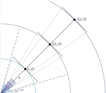
structures of the sequence. This algorithm can also work in annular mode, where an optimized PSF reference can be built for each annulus, taking into account a parallactic angle thresholdω for enforcing a given amount of field rotation in the reference frames. The thresholdω is defined as
r
2 arctan FWHM
2 , 1
w= d· ( )
where FWHM is the Gaussian full width at half maximum in pixels, δis a user-defined threshold parameter, and risthe angular separation for which the parallactic angle thresholdω is defined (see Figure1). The enhanced reference PSF is built for
each annulus by median combining the m closest in time frames, after discarding neighbor frames according to the threshold ω. Median reference PSF subtraction has limited performance in the small-angle regime, and it has been superseded by more advanced post-processing techniques.
4.2. PCA-based Algorithms for Reference PSF Subtraction PCA is aubiquitous method in statistics and data mining for computing the directions of maximal variance from data matrices. It can also be understood as a low-rank matrix approximation (Absil et al. 2008). PCA-based algorithms for
reference PSF subtraction on ADI data can be found in the VIP subpackage pca. For ADI-PCA, the reference PSF is constructed for each image by projecting the image onto a lower-dimensional orthogonal basis extracted from the data itself via PCA. Subtracting from each frame its reference PSF produces residual frames where the signal of the moving planets is enhanced. The most basic implementation of ADI-PCA uses all ofthe images by building a matrix MÎn´p, where n is the number of frames and pisthe number of pixels in a frame. The basic structure of the full-frame ADI-PCA algorithm is described in Appendix A along with details of VIP’s implementation. Also, VIP implements variations of the full-frame ADI-PCA tailored to reduce the comp-utation time and memory consumption when processing big datacubes(tens of GB in memory) without applying temporal
Figure 1.Illustration of the ADI rotation thresholds at different separations in D
l . The dotted–dashed lines show the rejection zone at2l Dwithδ = 1 that ensures a rotation by at least 1×FWHM ( Dl ) of the PSF.
frame sub-sampling(see AppendixBfor details). AppendixB
also showshow temporal sub-sampling can degrade the sensitivity of off-axis companions.
It is worth noting that, in VIP, a PCA-based algorithm can also be used for RDI datacubes, multiple-channel SDI datacubes, and IFS data with wavelength and rotational diversities. Data processing for RDI and SDI within VIP is on-going work and will not be described in more detail in this paper.
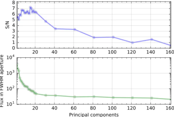
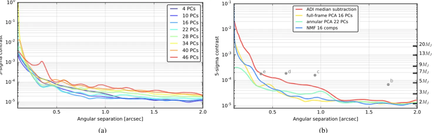
Optimizing k for ADI-PCA. The most critical parameter in every PCA-based algorithmis the number of principal components (PCs) k. VIP implements an algorithm to find the k that maximizes the S/N metric, described in Section2, for a given location in the image, by running a grid search varying the value of k and measuring the S/N for the given coordinates. This algorithm can also define an adaptative grid refinement to avoid computing the S/N in regions of the parameter space far from the maximum. This algorithm does not deal with the reliability of the candidate point source located at the coordinates of interest. The computational cost remains close to that of a single full-frame ADI-PCA run thanks to the fact that we compute the PCA basis once with the maximum k we want to explore. Having this basis, we truncate it for each k PCs in the grid and proceed to project, subtract, and produce the final frames where the S/N is computed. An example of such anoptimization procedure is shown in Figure2for the position of planet HR 8799e in the data set described in Section 7. In this case, we maximized the mean S/N in an FWHM aperture. We can observe that the optimal S/N reaches a plateau near the maximum. For true planets, the S/N decreases slowly when increasing the number of PCs, as shown in the top panel of Figure2, in contrast with a more abrupt S/N decay for noise artifacts or bright speckles (which have significant S/N only for a few PCs and quickly fade away). The maximum S/N does not correspond to the maximum algorithm throughput, and in the illustrated case occurs for a throughput of about 0.1.
Optimizing the library for ADI-PCA. Full-frame ADI-PCA suffers from companion self-subtraction when the signal of interest, especially that of a close-in companion, gets absorbed by the PCA-based low-rank approximation that models the reference PSF (Gomez Gonzalez et al. 2016a). A natural
improvement of this algorithm for minimizing the signal loss is the inclusion of a parallactic angle threshold for discarding
rows from M when learning the reference PSF. This frame selection for full-frame ADI-PCA is optional and can be computed for only one separation from the star. The idea is to leave in the reference library those frames where the planet has rotated by at least an angleω, as described in Section4.1. The computational cost increases when performing the selection of library frames(for each frame according to its index in the ADI sequence) since n singular value decompositions (SVD) need to be computed for learning the PCs of matrices with less rows than M. Following the same motivation of refining the PCA library, VIP implements an annular ADI-PCA algorithm, which splits the frames in annular regions (optionally in quadrants of annuli) and computes the reference PSF for each patch taking into account a parallactic angle rejection threshold for each annulus. This ADI-PCA algorithm processes n×nannuli(or 4n × nannuliin case quadrants are used) smaller matrices. Details about the annular ADI-PCA algorithm implementation can be found in AppendixC.
4.3. Non-negative Matrix Factorization(NMF) for ADI As previously discussed, the PCA-based low-rank approx-imation of an ADI datacube can be used to model the reference PSF for each one of its frames. In thefields of machine learning and computer vision, several approaches other than PCA have been proposed to model the low-rank approximation of a matrix (Kumar & Shneider 2016; Udell et al. 2016). In
particular, NMF aims tofind a k-dimensional approximation in terms of non-negative factors W and H (Lee & Seung1999).
NMF is distinguished from the other methods by its use of non-negativity constraints on the input matrix and on the factors obtained. For astronomical images, the positivity is guaranteed since the detector pixels store the electronic charge produced by the arriving photons. Nevertheless, the sky subtraction operation can lead to negative pixels in the background and in this case a solution is to shift all the values on the image by the absolute value of the minimum pixel, turning negative values into zeros.
NMF finds a decomposition of M into two factors of non-negative values, by optimizing for the Frobenius norm:
M WH M WH argmin1 2 1 2 , 2 W H F i j ij ij , 2 , 2
å
- = - ( ) ( )where WÎn´k, HÎk´p, and WH is a k-rank approx-imation of M. Such a matrix factorization can be used to
model a low-rank matrix based on the fact that
WH W H
rank( )min rank( ( ), rank( )), where rank(X) denotes the rank of a matrix X. Therefore, if k is small, WH is low-rank. NMF is a non-convex problem, and has no unique minimum. Therefore, it is a harder computational task than PCA, and no practical algorithm comes with a guarantee of optimality (Vavasis 2009). It is worth noting that this
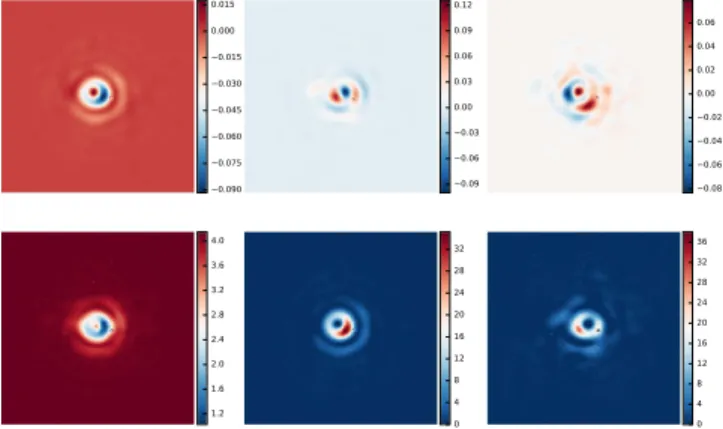
Frobenius-norm formulation of NMF, as implemented in scikit-learn, provides final images very similar to the ones from full-frame ADI-PCA. The first NMF components along with thefirst PCs for an identicaldata set are shown in Figure 3. The NMF components are strictly positive and the NMF-based low-rank approximation that models the refer-ence PSF for each frame is computed as a linear combination of these components. This NMF-based algorithm makes a
Figure 2.Top: grid optimization of the number of PCs for full-frame ADI-PCA at the location of the HR 8799e planet. In this example, the mean S/N in an FWHM aperture was maximized with 16 PCs. Bottom: flux of planet HR 8799e in an FWHM aperture in thefinal, post-processed image.
useful complement to PCA-based algorithms for testing the robustness of a detection.
4.4. LLSG for ADI
Very recently, a Local Low-rank plus Sparse plus Gaussian-noise decomposition (LLSG, Gomez Gonzalez et al. 2016a)
was proposed as an approach to enhance residual speckle noise suppression and improve the detectability of point-like sources in the final image. LLSG builds on recent subspace projection techniques and robust subspace models proposed in the computer vision literature for the task of background subtrac-tion from natural images, such as video sequences(Bouwmans & Zahzah 2014). The subpackage llsg contains an
implementation of the LLSG algorithm for ADI datacubes. Compared to the full-frame ADI-PCA algorithm, the LLSG decomposition reaches a higher S/N on point-like sources and has overall better performance in the receiver operating characteristic (ROC) space. The boost in detectability applies mostly to the small inner working angle region, where complex speckle noise prevents full-frame ADI-PCA from discerning true companions from noise. One important advantage of LLSG is that it can process an ADI sequence without increasingthe computational cost too much compared to the fast full-frame ADI-PCA algorithm. More details about LLSG and its performance can be found in Gomez Gonzalez et al. (2016a).
5. Flux and Position Estimation for ADI
VIP implements the negative fake companion technique (NEGFC, Lagrange et al. 2010; Marois et al. 2010) for the
determination of the position and flux of companions. This implementation is contained in the subpackage negfc. The NEGFC technique consists ofinjecting in the sequence of frames a negative PSF template with the aim of canceling out the companion as well as possible in the final post-processed image. The PSF template is obtained from off-axis observations of the star. Injecting this negative PSF template directly in the images, before they are processed, allows us to take into account the biases in photometry and astrometry induced by the post-processing algorithms. The best cancellation of the companion PSF is achieved by minimizing, in an iterative
process, a well-chosenfigure of merit:
f I , 3 i P i 1
å
= = ∣ ∣ ( )where P represents the pixels contained in a circular aperture (of variable radius, by default 4 × FWHM) centered on the companion in the final collapsed post-processed image. This NEGFC function of merit can be tweakedby changing the default parameters of the VIP’s NEGFC procedure. Optionally, one can minimize the standard deviation of the pixels, instead of the sum. According to our test, minimizing the standard deviation is better in cases when the companion is located in a region heavily populated by speckles(close to the star). Also, it is possible to use the pixels from each residual frame, thus avoiding collapsing the datacube in a singlefinal frame. Using the n×P pixels from the residual cube helps remove any bias that the collapsing method, andby default a median combina-tion of the frames, may introduce.
In VIP, the estimation of the position and flux (three parameters: radius R, theta θ,and flux F) is obtained by performing three consecutive procedures. Afirst guess of the flux of a companion is obtained by injecting an NEGFC in the calibrated frames, whilefixing R and θ and evaluating the function of merit for a grid of possible fluxes. This initial position(R and θ) is determined by visual inspection of final post-processed frames or based on prior knowledge. The first guess of the companion position/flux can be refined by performing a downhill simplex minimization (Nelder & Mead 1965), where the three parameters of the NEGFC are
allowed to vary simultaneously. Although the simplex mini-mization leads to a significant improvement of the position/ flux determination, it does not provide error bars on the three estimated parameters. More importantly, the function of merit of the NEGFC technique is not strictly convex and finding a global minimum is not guaranteed. Our approach in VIP is to turn our minimization function of merit into a likelihood and to use Monte Carlo methods for sampling the posterior probability density functions(PDF) for R, θ, and F. This can be achieved via Nested Sampling, calling the nestle library,18or Markov Chain Monte Carlo (MCMC), through the emcee (Foreman-Mackey et al. 2013) package,which implements an
affine-invariant ensemble sampler for MCMC. The position andflux obtained with the simplex minimization are used for initializing the Monte Carlo procedures. From the sampled parame-terPDFs, we can infer error bars and uncertainties in our estimations, at the cost of longer computation time. This NEGFC implementation in VIP currently works with ADI-PCA-based post-processing algorithms. We also include a procedure for estimating the influence of speckles in the astrometric and photometric measurements, based on the injection of fake companions at various positions in the field of view. More details on the NEGFC technique, the definition of the confidence intervals, and details about the speckle noise estimation can be found in Wertz et al. (2016), where this
procedure is used to derive robust astrometry for the HR 8799 planets.
Figure 3.First three principal(top row) and NMF components (bottom row). The components of NMF are strictly positive. Thisfigure is better visualized in color.
18
6. Sensitivity Limits
Sensitivity limits (in terms of planet/star contrast), often referred to as contrast curves, are commonly used in the literature for estimating the performance of high-contrast direct imaging instruments. They show the detectable contrast for point-like sources as a function of the separation from the star. VIPfollows the current practice in building sensitivity curves from Mawet et al. (2014) and thereby applies a student-t
correction to account for the effect of the small sample statistics. This correction imposes a penalty at small separations and therefore the direct comparison with contrast curves from previous works may seem more pessimistic close to the parent star. The function, contained in the subpackage phot, requires an ADI data set, a corresponding instrumental PSF, and the stellar aperture photometry Fstar. We suggest removing any real, high-significance companions from the datacube (for example, using the NEGFC approach) before computing a contrast curve. The first step is to measure the noise as a function of the angular separationσR, on afinal post-processed frame from the ADI datacube, by computing the standard deviation of thefluxes integrated in FWHM apertures. Then we inject fake companions to estimate empirically the throughput TRof the chosen algorithm(i.e., the signal attenuation) at each angular separation as TR = Fr/Fin, where Fris the recovered flux of a fake companion after the post-processing and Finis the initially injected flux of the fake companion. We define the contrast CRas C k T F , 4 R R R star s = · · ( )
where k is a factor,five in case we want the five sigma contrast curve, corrected for the small sample statistics effect. The transmission of the instrument, if known, can be optionally included in the contrast calculation.
We note that contrast curves depend on the post-processing algorithm used and its tuning, as will be shown in the panel(a) of Figure 7. In signal detection theory, the performance of a detection algorithm is quantified using ROC analysis, and several meaningful figures of merit can be derived from it (Barrett et al. 2006; Gomez Gonzalez et al. 2016a). These
figures of merit would be better suited than sensitivity curves for post-processing algorithmperformance comparison. We only provide contrast curve functionality in VIP as the proper computation and the use of ROC curves is asubject of on-going research.
7. Applying VIP to On-sky Data
We will now proceed to showcase VIP on a data set of HR 8799, a young A5V star located at 39 pc, hosting a multiple-planet system and a debris disk (Marois et al.2008). Its four
planets are located at angular separations ranging from about 0 4 to 1 7, and have masses ranging from 7 to 10 MJ(Currie et al.2011). The HR 8799 data set used in the present work was
obtained at the Large Binocular Telescope (LBT, Hill et al.2014) on 2013 October 17, during the first commissioning
run of the L′-band annular groove phase mask (AGPM) on the LBT Interferometer (LBTI, Defrère et al. 2014; Hinz et al.
2014). A deep ADI sequence on HR 8799 was obtained in
pupil-stabilized mode on the LBTI’s L and M Infrared Camera (LMIRCam), equipped with its AGPM coronagraph, using only the left-side aperture. The observing sequence lasted for
approximately 3.5 hr, providing a field rotation of 120° and resulting in ∼17000 frames on target. The seeing was fair during the first 30 minutes (1 2–1 4) and good for the remaining observations (0 9–1 0). The adaptive optics loop was locked with 200 modesfirst and with 400 modes after 30 minutes. The off-axis PSF was regularly calibrated during the observations by placing the star away from the AGPM center (Defrère et al. 2014). The raw sequence of frames was flat
fielded and background subtracted with custom routines. The sky background subtraction was performed using the median combination of close-in time sky frames. Using a master bad pixel mask generated with sky frames taken at the end of the night, the bad pixels were subsequently fixed in each frame using the median of adjacent pixels(Defrère et al.2014).
7.1. Data Processing with VIP
The calibrated datacube was loaded in memory with VIP and re-centered using as a point of reference a ghost PSF present in each frame, created by a secondary reflection in the LBTI trichroic(Defrère et al. 2014; Skemer et al. 2014). The
offset between the secondary reflection and the central source was measured on the non-saturated PSF observations via 2D-Gaussian fits. VIP includes a function for aligning frames by fitting a frame region with a 2D-Gaussian profile (using Astropyfunctionality). We used this function for fitting the secondary reflection on each frame and placing the star at the center of odd-sized square images taking into account the previously calculated offset between the reflection and the main beam.
For the bad framerejection step, we used the VIP’s algorithm based on the linear correlation of each frame with respect to a reference from the same sequence (30×30 centered sub-frames are used). The reference frame was chosen by visual inspection and in agreement with the observing log of the adaptive optics system. Ten percent of the frames were finally discarded resulting in a datacube with size 15254×391×391 (after cropping the frames to the region of interest), occupying 9.7 GB of disk space (in single float precision).
The workflow for loading data in memory and pre-processing it with VIP is as follows.
1 import vip 2
3# loading the calibrated datacube and 4# parallactic angles
5 cube= vip.fits.open_fits(“path_cube”) 6 pa= vip.fits.open_fits(“path_pa”) 7
8# aligning the frames
9 from vip.calib import cube_recenter_gauss2d_fit⧹ 10 as recenter
11 cube_rec= recenter(cube, xy = cent_subim_fit, 12 fwhm= fwhm_lbt, subi_size = 4, 13 offset= offset_tuple, debug = False) 14
15# identifying bad frames
16 from vip.calib import cube_detect_badfr_correlation⧹ 17 as badfrcorr
18 gind, bind= badfrcorr(cube_rec, frame_ref = 9628, 19 dist= “pearson”, percentile = 10, plot = False) 20
21# discarding bad frames
(Continued) 23
24# cropping the re-centered frames 25 from vip.calib import cube_crop_frames
26 cube_gf_cr= cube_crop_frames(cube_gf, size = 391)
Afirst exploration of the resolution datacube with full-frame ADI-PCA showed a feature that resembled an instru-mental PSF near the location of planet HR 8799e, when only a few PCs were used (see theleft panel in Figure 4). We
concluded, after processing the data in two halves, that this blob was a residual artifact of the secondary reflection of LBTI, which left a PSF-like footprint due to the slow rotation in the first third of the sequence. The ghost companion appeared very bright when using thefirst half of the sequence and was totally absent using the second one, as shown in Figure4. Moreover, it was located at the same separation as the secondary reflection, whose offset was previously measured. For this reason, and because the adaptive optics system was locked on 200 modes during thefirst 5000 frames, while it locked on 400 modes for the rest of the sequence, we discarded thisfirst batch of frames from the sequence and kept the frames with the highest quality. The rotation range of thefinal sequence is 100°, and the total on-source time amounts to 2.8 hr.
We processed this datacube with several ADI algorithms, and tuned their parameters for obtaining final frames of high quality, where we investigated the presence of a potentialfifth companion. Other than the four known planets around HR 8799, we did not find any significant detection, worth further investigation. With the sole purpose of saving time while showcasing the VIP functionalities, we then decided to sub-sample temporally our ADI sequence by mean combining every 20 frames, and thereby obtained a datacube of 499 frames. We refrained from binning the pixels and worked with the over-sampled LMIRCam images featuring an FWHM of nine pixels. The code below illustrates how thesesteps where done with VIP.
1# temporal sub-sampling of frames 2# mean combination of every 20 frames 3 from vip.calib import cube_subsample
4 cube_ss, pa_ss= cube_subsample(cube_gf[5000:], 5 n= 20, mode = “mean”, parallactic = pa_gf[5000:]) 6
7# cube_ss is a 3D numpy array with shape 8# [499, 391, 391] and pa_ss a vector [499] 9# with the corresponding paralactic angles 10
11# ADI median subtraction using 2XFWHM annuli, 12# 4 closest frames and PA threshold of 1 FWHM
(Continued) 13 fr_adi= vip.madi.adi(cube_ss, pa_ss, 14 fwhm= fwhm_lbt, mode = “annular”, 15 asize= 2, delta_rot = 1, nframes = 4) 16
17# post-processing using full-frame ADI-PCA 18 fr_pca= vip.pca.pca(cube_ss, pa_ss, ncomp = 10) 19
20# fr_adi and fr_pca are 2d numpy arrays with 21# shape [391, 391]
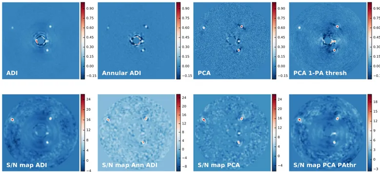
Figures 5 and 6 show a non-exhaustive compilation of the ADI post-processing options with varying parameters. All of the algorithms were set to mask the innermost2l Dregion.
We observe how more complex PSF subtraction techniques outperform the classic median subtraction approach for cleaning the innermost part of the image(∼2λ/D). We refrain from deriving additional conclusions about the comparison of different post-processing techniques, asthis is beyond the scope of this paper. Furthermore, this is an exercise to be carried out using a diverse collection of data sets (from different instruments) and with appropriate metrics (defined by the whole community), such as the area under the ROC curve, in order to provide general and robust conclusions. We envision VIP as a library that could eventually implement all the main high-contrast imaging algorithms and become a tool suitable for benchmarking different data processing approaches under a unified open framework.
7.2. Sensitivity Limits and Discussion
The code below shows how to compute the S/N for a given resolution element, obtain an S/N map, call the NEGFC MCMC function, and compute a contrast curve.
1 from vip.phot import snr_ss, snrmap, 2 contrast_curve
3 snr_value= snr_ss(fr_pca, source_xy = (54,266),
4 fwhm= fwhm_lbt) 5 6# S/N map generation 7 snr_map= snrmap(fr_pca, fwhm = fwhm_lbt, 8 plot= True) 9 10# NEGFC mcmc sampling
11 from vip.negfc import mcmc_negfc_sampling, 12 confidence, cube_planet_free
13 ini_rad_theta_flux = np.array([r_0, th_0, f_0]) 14 chain= mcmc_negfc_sampling(cube_ss, pa_ss, 15 psfn= psf, ncomp = 8, plsc = pxscale_lbt, 16 fwhm= fwhm_lbt, initialState = ini_rad_theta_flux, 17 nwalkers= 100, niteration_min = 100,
18 niteration_limit= 400, nproc = 10) 19
20# 1-sigma confidence interval calculation 21# from the mcmc chain
22 val_max, conf= confidence(chain, cfd = 68, 23 gaussianFit= True, verbose = True) 24 final_rad_theta_flux = [(r, theta, f)]
25 cube_emp= cube_planet_free(final_rad_theta_flux, 26 cube_ss, pa_ss, psfn= psf, plsc = pxscale_lbt) 27
28# res_cc is a (pandas) table containing the 29# constrast, the radii where it was evaluated, 30# the algorithmic throughput and other values 31 res_cc= contrast_curve(cube_emp, pa_ss, Figure 4.Ghost planet(shown with an arrow) due to the secondary reflection
of LBTI. The left panel shows the full-frame ADI-PCA result using six PCs on the whole ADI sequence. The middle and right panels show the same processing but using only thefirst and second halves of the sequence.
(Continued) 32 psf_template= psf, fwhm = fwhm_lbt, 33 pxscale= pxscale_lbt, starphot = starphot,
34 sigma= 5, nbranch = 1, algo = vip.pca.pca, ncomp = 8)
Using the NEGFC technique, we subtracted the four known companions in our datacube and computed the sensitivity curves on this empty datacube. Panel(a) of Figure7shows the 5σ sensitivity for full-frame ADI-PCA with varying PCs to exemplify the dependence on the algorithm parameters. By using VIP’s ADI-PCA algorithm in its annular mode and setting a different number of PCs for each separation, we could obtain the optimal contrast curve, as already shown by Meshkat et al.(2014). Panel (b) of Figure7shows the 5σ sensitivities for the available ADI algorithms in VIP. These sensitivity limits should be representative of the expected performance of the algorithms when applied to different data, but the result may vary, therefore preventing us from presenting more general conclusions. As expected, in panel(b) of Figure7, we observe how the median reference PSF subtraction achieves worse contrast than the rest of the algorithms. Also, we see that with annular ADI-PCA, impressive contrast is achieved at small separations (below 0 5) and similar contrast at larger separations if it is compared to full-frame ADI-PCA. Annular ADI-PCA presents a smaller dependence on the number of PCs (the variance of the contrast curves, when varying k, is smaller compared to full-frame ADI-PCA). For the full-frame ADI-NMF sensitivity, we used 16 components as in the case of full-frame ADI-PCA and obtained a fairly similar performance at all separations. The contrast metric, as defined in VIP, is not well adapted to all algorithms and/or data sets;therefore, we refrain from presenting such asensitivity curve for LLSG. Recall that these contrast curves were obtained on a temporally sub-sampled datacube. However, because we do not include time-smearing when injecting fake companions, we expect the
results to be representative of the ultimate sensitivity based on the full(non-sub-sampled) ADI sequence. The contrast-to-mass conversion for the HR 8799 planets was obtained assuming an age of 40 Myr(Bowler2016) and using the 2014 version of the
PHOENIX BTSETTL models for substellar atmospheric models described in Baraffe et al. (2015). Based on this, we
can discard the presence of afifth planet as bright as HR 8799e down to an angular separation of 0 2. Our detection limits remain in the planetary-mass regime down to our inner working angle of 0 1, and reach a background-limited sensitivity of 2 MJbeyond about 1 5.
Finally, it is worth mentioning that the full-frame ADI-PCA sensitivity curve presented in this paper (see yellow curve in the panel(b) of Figure7) is slightly worse than the one shown
in Maire et al. (2015) and obtained four days later with the
same instrument but without the AGPM coronagraph. In order to make a fair comparison, we re-processed this data set with VIP and obtained the same results as Maire et al. (2015) at
large angular separations but more pessimistic results closer in (within 0 5). This can be explained by the student-t correction that we apply. If we compare the contrast curves produced by VIP for both data sets, we observe that at small angular separations, within 1″, the AGPM coronagraph provides an improvement in contrast up to 1 magnitude.
8. Summary
In this paper, we have presented the VIP package for data processing of astronomical high-contrast imaging data. It has been successfully tested on data coming from a variety of instruments, i.e., Keck/NIRC2, VLT/NACO, VLT/VISIR, VLT/SPHERE, and LBT/LMIRCam, thanks to our effort of developing VIP as aninstrument-agnostic library. VIP imple-ments functionalities for processing high-contrast imaging data at every stage, from pre-processing procedures to contrast curvecalculations. Concerning the post-processing capabilities
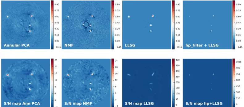
Figure 5.Post-processingfinal frames (top row) and their corresponding S/N maps (bottom row) for classical ADI, annular ADI, full-frame ADI-PCA, and full-frame ADI-PCA with a parallactic angle threshold. Thefinal frames have been normalized to their own maximum value. No normalization or scaling was applied to the S/N maps, which feature their full range of values.
of VIP for the case of ADI data, it includes several types of low-rank matrix approximations for reference PSF subtraction, such as the LLSG decomposition, and PCA- and NMF-based algorithms. We present, as one of several PCA enhancements, an incremental ADI-PCA algorithm capable of processing big, larger-than-memory ADI data sets. In this work, we also showcased VIP’s capabilities for processing ADI data, using a long sequence on HR 8799 taken with LBTI/LMIRCam in its AGPM coronagraphic mode. We used all of VIP’s capabilities to investigate the presence of a potential fifth companion around HR 8799, but we did notfind any significant additional point-like sources. Further development of VIP is plannedin order to improve its robustness and efficiency (for supporting big data sets in every procedure and multi-processing), and add more state-of-the-art algorithms for high-contrast imaging data processing. We propose VIP not as an ultimate solution to all high-contrast image processing needs, but as an open science exercise hoping that it will attract more users and in turn be developed by the high-contrast imaging community as a whole.
The authors would like to thank the whole python source community and the developers of the powerful open-source stack of scientific libraries. Special thanks to the creators of the Ipython Jupyter19application. We also thank Elsa Huby, Maddalena Reggiani,and Rebecca Jensen-Clem for useful discussions and early bug reports. Finally, we thank the referee, Tim Brandt, for his constructive questions and valuable comments. The research leading to these results has received funding from the European Research Council Under the European Union’s Seventh Framework Program (ERC Grant Agreement n. 337569) and from the French Community of Belgium through an ARC grant for Concerted Research Action. V.C. acknowledges financial support provided by Millennium Nucleus grant RC130007(Chilean Ministry of Economy). The LBTI is funded by the National Aeronautics and Space
Administration as part of its Exoplanet Exploration Program. The LBT is an international collaboration among institutions in the United States, Italy, and Germany. LBT Corporation partners areThe University of Arizona on behalf of the Arizona university system; Instituto Nazionale di Astrofisica, Italy; LBT Beteiligungsgesellschaft, Germany, representing the Max-Planck Society, the Astrophysical Institute Potsdam, and Heidelberg University; The Ohio State University, and The Research Corporation, on behalf of The University of Notre Dame, University of Minnesota and University of Virginia. This research was supported by NASA’s Origins of Solar Systems Program, grant NNX13AJ17G.
Software: numpy (van der Walt et al. 2011), scipy (Jones
et al. 2001), matplotlib (Hunter 2007), astropy (Astropy
Collaboration et al. 2013), photutils (Bradley et al. 2016),
scikit-learn(Pedregosa et al.2011), pandas (McKinney2010),
scikit-image (van der Walt et al. 2014), emcee
(Foreman-Mackey et al. 2013), OpenCV (Bradski 2000), SAOImage
DS9, nestle.
Appendix A
Details on the Full-frame ADI-PCA Algorithm The basic structure of the full-frame ADI-PCA algorithm is as follows.
1. The datacube is loaded in memory and M is built by storing on each row a vectorized version of each frame; 2. optionally M is mean centered or standardized
(mean-centering plus scaling to unit variance);
3. kmin(n, p) PCs are chosen to form the new basis B; 4. the low-rank approximation of M is obtained as MBTB,
which models the reference PSF for each frame; 5. this low-rank approximation is subtracted from M and the
result is reshaped into a sequence of frames; and 6. all residual frames are rotated to a common north and are
median combined in afinal image.
Figure 6.Same as Figure5for annular ADI-PCA, full-frame ADI-NMF, LLSG, and high-passfiltering coupled with LLSG. We note that a high S/N does not translate into increased sensitivity to fainter companions.
19
The PCs can be obtained by computing the eigen decomposi-tion(ED) and choosing the eigenvectors corresponding to the k largest eigenvalues of the covariance matrix MTM, or equivalently by computing the SVD of M and extracting the k dominant right singular vectors.
Instead of computing the ED of MTM (which is a large square matrix p× p that must fit in working memory) we can perform the ED of MMTfor a cheaper PCA computation. In a similar way, taking the SVD of MTis faster and yields the same result as computing the SVD of M. Both speed tricks are implemented in VIP. Python, as well as other modern programming environments, such as Mathematica, R, Julia and Matlab, relies on LAPACK (Linear Algebra PACKage),20which is the state-of-the-art implementation of numerical dense linear algebra. We use the Intel MKL libraries, which provide multi-core optimized high performance LAPACK functionality consistent with the standard. For the SVD, LAPACK implements a “divide-and-conquer” algorithm that splits the task of a big matrix SVD decomposition into some smaller tasks, achieving good performance and high accuracy when working with big matrices(at the expense of a large memory workspace).
Appendix B
Full-frame ADI-PCA for Big ADI Data Sets The size of an ADI data set may vary from case to case and depends on the observing strategy and the pre-processing steps taken. Typically, a datacube contains several tens to several thousands of frames, each one of typically 1000×1000 pixels for modern detectors used in high-contrast imaging. In selected instruments (VLT/NACO, LBTI/LMIRCam) that are able to record high-frame rate cubes, a two-hour ADI sequence can contain up to∼20,000 frames. After cropping down the frames to 400×400 pixels, we get a datacube in single float values occupying more than 10 GB of disk space. Loading this data set at once in memory, for building M, would not be possible on typical personal computer. Even if we manage to load the file, the PCA algorithm itself requires more RAM memory for SVD/ED calculations, which will eventually cause slowdowns (or system crashes) due to heavy disk swapping.
The most common approach for dealing with big data sets of this kind is to temporally and/or spatially sub-sample the
frames. Reducing the size of the data set effectively reduces the computation time of full-frame ADI-PCA to a few seconds but at the cost of smearing out the signal(depending on the amount of rotation). Also, depending on the temporal window used for co-adding the frames and on the PSF decorrelation rate, we might end up combining sections of the sequence where the PSF has a very different structure. It has been stated that there is an optimal window for temporal sub-sampling, which results in anincreased S/N (Meshkat et al. 2014). After running
simulations with fake companion injections at different angular separations and measuring the obtained mean S/N in al D aperture, we came to the conclusion that using the whole sequence of frames(data without temporal sub-sampling) is the best choice and delivers the best results in terms of S/N. For this test, we used a datacube of∼10,000 frames, each with 0.5 seconds of integration time. In panel(a) of Figure8, we show the S/N of the recovered companions in datacubes sub-sampled using different windows, for an arbitrarily fixed number of 21 PCs (even though 21 PCs do not necessarily represent the same explained variance for datacubes with different numbers of frames). There is an agreement with these results and those in Meshkat et al. (2014) for sub-sampling
windows larger than 20, but unfortunately Meshkat et al. (2014) did not consider smaller sub-sampling windows nor the
full ADI sequence. More information can be found in panel(b) of Figure 8, which shows the dependence of the fake companions S/N on the number of PCs for different angular separations. Our simulations show avery significant gain in S/N when temporal sub-sampling of frames is avoided, especially at large separations where smearing effects are the largest.
VIP offers two additional options when it comes to computingthe full-frame ADI-PCA through SVD, tailored to reduce the computation time and memory consumption when data sub-sampling needs to be avoided(see Figure 9). These
variations rely on the machine learning library Scikit-learn. The first is ADI-PCA through randomized SVD (Halko et al. 2011), which approximates the SVD of M by
using random projections to obtain k linearly independent vectors from the range of M, then uses these vectors tofind an orthonormal basis for it and computes the SVD of M projected to this basis. The gain resides in computing the deterministic SVD on a matrix smaller than M but with strong bounds on the quality of the approximation(Halko et al.2011).
Figure 7.(a) 5σ sensitivity (with the small sample statistics correction) for full-frame ADI-PCA with different numbers of PCs. (b) 5σ sensitivities for some of theADI algorithms in VIP. The four known companions were removed before computing these contrast curves. The small sample statistics correction has been applied to these sensitivities.
20
The second variation of the ADI-PCA uses the incremental PCA algorithm proposed by Ross et al.(2008), as an extension
of the Sequential Karhunen-Loeve Transform (Levy & Lindenbaum 2000), which operates in online fashion instead
of processing the whole data at once. For the ADI-PCA algorithm through incremental PCA, the FITSfile is opened in memmaping mode, which allows accessing small segments without reading the entirefile into memory, thus reducing the memory consumption of the procedure. Incremental PCA works by loading the frames in batches of size b and initializes the SVD internal representation of the required lower-dimensional subspace by computing the SVD of the first batch. Then it sequentially updates n/b times the PCs with each new batch until all the data is processed. Once thefinal PCs are obtained, the same n/b batches are loaded once again and the reconstruction of each batch of frames is obtained and subtracted for obtaining the residuals, which are then de-rotated and median collapsed. Afinal frame is obtained as the median of the n/b median collapsed frames. A similar approach to incremental PCA, focusing on covariance update, has been proposed by Savransky (2015). In Figure 9,the memory consumption and total CPU time are comparedfor all the variants of full-frame ADI-PCA previously discussed. These tests were performed using a 10 GB(on disk) sequence and on a workstation with 28 cores and 128 GB of RAM. The results show how incremental PCA is the lightest on memory usage while randomized PCA is the fastest method. With incremental PCA, an appropriate batch size can be used for fitting in memory datacubes that otherwise would not, without sacrificing the accuracy of the result.
Appendix C Annular ADI-PCA
The annular ADI-PCA comprises the following steps. 1. The datacube is loaded in memory, the annuli are
constructed, and a parallactic angle threshold is computed for each one of them;
2. for each annulus, a matrix M n p
annulusδannulus is built;
3. optionally Mannulusis mean centered or standardized; 4. for each frame and according to the rotation threshold, a
new Moptmatrix is formed by removing adjacent rows; Figure 8. (a) Fake companion’s S/N for different angular separations as
a function of the temporal sub-sampling applied to the ADI sequence. The horizontal axis shows the amount of frames that were mean combined, with zero meaning that the whole ADI sequence(10k frames) is used. Full-frame ADI-PCA is applied on each datacube, with 21 PCs.(b) Retrieved S/N on fake companions injected at different angular separations and with a constant flux. The top panel shows the results of varying the number of principal components of the full-frame ADI-PCA algorithm when processing the full-resolution ADI sequence. The rest of the panels show the same S/N curves obtained on sub-sampled versions of the sequence using different windows.
Figure 9.Memory usage as a function of the processing time for different variations of the full-frame ADI-PCA algorithm on a large datacube(20 PCs were requested). This is valid for datacubes occupying several GB on disk (in this particular case,a 10 GB FITS file was used). It is worth noting that for short or sub-sampled ADI sequences the full-frame ADI-PCA through LAPACKSVD is very efficient and the difference in processing time may become negligible.
5. from Mopt,the kmin(nopt, pannulus) PCs are chosen to form the new basis optimized for this annulus and this frame;
6. the low-rank approximation of the annulus patch is computed and subtracted;
7. the residuals of this patch are stored in a datacube of residuals, which is completed when all the annuli and frames are processed; and
8. the residual frames are rotated to a common north and median combined in a final image.
This algorithm has been implemented with multi-processing capabilities allowing usto distribute the computations on each zone separately. According to our experience, using more than four cores for the SVD computation (through LAPACK/MKL) of small matrices, like the ones we produce in the annular ADI-PCA, does not lead to increased performance due to the overhead in the multi-threading parallelism. When used on a machine with a large number of cores, this algorithm can be set to process each zone in parallel, coupling both parallelisms for higher speed performance. Computing the PCA-based low-rank approximation for smaller patches accounts for different pixel statistics at different parts of the frames. This algorithm can also automatically define the parameter k for each patch by minimizing the standard deviation in the residuals, similar to the objective of the original LOCI algorithm (Lafrenière et al.2007), at the expense of an increased computation time.
References
Absil, P.-A., Mahony, R. E., & Sepulchre, R. 2008, Optimization Algorithms on Matrix Manifolds, I–XIV (Princeton, NJ: Princeton Univ. Press) 1–224 Amara, A., & Quanz, S. P. 2012,MNRAS,427, 948
Astropy Collaboration, Robitaille, T. P., Tollerud, E. J., et al. 2013, A&A, 558, A33
Baraffe, I., Homeier, D., Allard, F., & Chabrier, G. 2015,A&A,577, A42 Barrett, H. H., Myers, K. J., Devaney, N., Dainty, J. C., & Caucci, L. 2006,
Proc. SPIE,6272, 62721W
Bouwmans, T., & Zahzah, E.-H. 2014, Computer Vision and Image Understanding, 122, 22
Bowler, B. P. 2016,PASP,128, 102001
Bradley, L., Sipocz, B., Robitaille, T., et al. 2016, astropy/photutils, v0.3, Zenodo, doi:10.5281/zenodo.164986
Bradski, G. 2000, Dr Dobb’s Journal of Software Tools
Brandt, T. D., McElwain, M. W., Turner, E. L., et al. 2013,ApJ,764, 183 Cantalloube, F., Mouillet, D., Mugnier, L. M., et al. 2015,A&A,582, A89 Currie, T., Burrows, A., Itoh, Y., et al. 2011,ApJ,729, 128
Defrère, D., Absil, O., Hinz, P., et al. 2014,Proc. SPIE,9148, 91483X De Rosa, R. J., Rameau, J., Patience, J., et al. 2016,ApJ,824, 121
Foreman-Mackey, D., Hogg, D. W., Lang, D., & Goodman, J. 2013,PASP, 125, 306
Gomez Gonzalez, C. A., Absil, O., Absil, P.-A., et al. 2016a, A&A, 589, A54
Gomez Gonzalez, C. A., Wertz, O., Christiaens, V., Absil, O., & Mawet, D. 2015, VIP: Vortex Image Processing Package for High-Contrast Direct Imaging, v.0.7.0, Zenodo, doi:10.5281/zenodo.573261
Gomez Gonzalez, C. A., Wertz, O., Christiaens, V., Absil, O., & Mawet, D. 2016b, VIP: Vortex Image Processing pipeline for high-contrast direct imaging of exoplanets, Astrophysics Source Code Library, ascl:1603.003 Guizar-Sicairos, M., Thurman, S. T., & Fienup, J. R. 2008,OptL,33, 156 Guyon, O. 2005,ApJ,629, 592
Halko, N., Martinsson, P.-G., & Tropp, J. A. 2011,SIAMR, 53, 217 Hill, J. M., Ashby, D. S., Brynnel, J. G., et al. 2014,Proc. SPIE, 9145, 914502 Hinz, P., Bailey, V. P., Defrere, D., et al. 2014, in, 91460T-91460T-10 Hunter, J. D. 2007,CSE,9, 90
Jones, E., Oliphant, T., Peterson, P., et al. 2001, SciPy: Open source scientific tools for Python
Kumar, N. K., & Shneider, J. 2016,Linear and Multilinear Algebra, 1 Lafrenière, D., Marois, C., Doyon, R., Nadeau, D., & Artigau, É. 2007,ApJ,
660, 770
Lagrange, A.-M., Bonnefoy, M., Chauvin, G., et al. 2010,Sci,329, 57 Lee, D. D., & Seung, H. S. 1999,Natur,401, 788
Levy, A., & Lindenbaum, M. 2000,ITIP,9, 1371
Maire, A.-L., Skemer, A. J., Hinz, P. M., et al. 2015,A&A,576, A133 Marois, C., Lafrenière, D., Doyon, R., Macintosh, B., & Nadeau, D. 2006,ApJ,
641, 556
Marois, C., Macintosh, B., Barman, T., et al. 2008,Sci,322, 1348 Marois, C., Macintosh, B., & Véran, J.-P. 2010,Proc. SPIE,7736, 77361J Mawet, D., Milli, J., Wahhaj, Z., et al. 2014,ApJ,792, 97
Mawet, D., Pueyo, L., Lawson, P., et al. 2012,Proc. SPIE,8442, 844204 McKinney, W. 2010, in Proc. 9th Python in Science Conf., ed.
S. van der Walt & J. Millman, 51
Meshkat, T., Kenworthy, M. A., Quanz, S. P., & Amara, A. 2014,ApJ,780, 17 Mugnier, L. M., Cornia, A., Sauvage, J.-F., et al. 2009,JOSAA,26, 1326 Nelder, J. A., & Mead, R. 1965,Computer Journal, 7, 308
Oppenheimer, B. R., & Hinkley, S. 2009,ARA&A,47, 253
Pedregosa, F., Varoquaux, G., Gramfort, A., et al. 2011, Journal of Machine Learning Research, 12, 2825
Pepe, F., Ehrenreich, D., & Meyer, M. R. 2014,Natur,513, 358 Pueyo, L., Soummer, R., Hoffmann, J., et al. 2015,ApJ,803, 31
Ross, D. A., Lim, J., Lin, R.-S., & Yang, M.-H. 2008,International Journal of Computer Vision, 77, 125
Savransky, D. 2015,ApJ,800, 100
Skemer, A. J., Hinz, P., Esposito, S., et al. 2014, Proc. SPIE, 9148, 91480L
Soummer, R., Pueyo, L., & Larkin, J. 2012,ApJL,755, L28
Udell, M., Horn, C., Zadeh, R., & Boyd, S. P. 2016,Foundations and Trends in Machine Learning, 9, 1
van der Walt, S., Colbert, S. C., & Varoquaux, G. 2011,CSE, 13, 22 van der Walt, S., Schönberger, J. L., Nunez-Iglesias, J., et al. 2014,PeerJ,
2, e453
Vavasis, S. A. 2009,SIAM Journal on Optimization, 20, 1364
Wertz, O., Absil, O., Gómez González, C. A., et al. 2016,A&A,598, A83 Wilson, G., Aruliah, D. A., Brown, C. T., et al. 2014,PLoS Biol, 12, e1001745