Accelerated and Localized Newton Schemes for
Faster Dynamic Simulation of Large Power Systems
Davide Fabozzi, Student, IEEE
Angela S. Chieh, Member, IEEE
Bertrand Haut
Thierry Van Cutsem, Fellow, IEEE
Abstract—This paper proposes two methods to speed up
the demanding time-domain simulations of large power system models. First, the sparse linear system to solve at each Newton iteration is decomposed according to its bordered block diagonal structure, in order to solve only those parts that need to be solved, and update only sub-matrices of the Jacobian that need to be updated. This brings computational savings without degradation of accuracy. Next, the Jacobian structure is further exploited to localize the system response, i.e. involve only the components identified as active, with an acceptable and controllable decrease in accuracy. The accuracy and computational savings are assessed on a large-scale test system.
Index Terms—time simulation, large-scale systems,
differential-algebraic equations, Newton method, bordered block diagonal matrices, Schur complement, localization
I. INTRODUCTION
D
YNAMIC simulations are routinely used to check the response of electric power systems to large disturbances [1], [2]. In spite of the increase in computational power, simulation of large-scale systems remains time consuming. Indeed, they require solving a large set of nonlinear stiff hybrid differential-algebraic equations. A large interconnected system may involve hundreds of thousands of such equations spanning very different time scales and undergoing many discrete transitions.Dynamic Security Assessment (DSA) is one application impacted by this computational burden [3]. This is even more true when, instead of the 10 to 20 seconds simulated for short-term stability, the evolution is computed until a new steady state is reached, which requires simulating long-term dynamics over several minutes after the initiating event.
This computational burden justifies the fact that many control centers routinely perform static security assessment, typically AC (if not DC for some problems) power flows and resort infrequently to DSA. However, the need for DSA is ex-pected to go increasing. Indeed, operation of non-expandable grids closer to their stability limits and unplanned generation patterns stemming from renewable energy sources require dynamic studies. Furthermore, under the pressure of electricity D. Fabozzi and T. Van Cutsem are with the Department of Electrical Engineering and Computer Science (Montefiore Institute) of the University of Li`ege, Sart Tilman B37, B-4000 Li`ege, Belgium. A.S. Chieh is with the R&D department of RTE (the French transmission system operator), 78000 Versailles, France. B. Haut is with Tractebel Engineering, B-1000, Brussels, Belgium. T. Van Cutsem is with the Fund for Scientific Research (FNRS). This work was performed in the context of the PEGASE project funded by European Community’s 7th Framework Programme (grant agreement No. 211407).
markets and with the support of active demand response, it is likely that system security will be more and more guaranteed by emergency controls responding to the disturbance. In this context, security analysis requires checking the sequence of events that take place after the initiating disturbance, a task for which static calculation of the operating point in a guessed final configuration is inappropriate.
While similar needs for faster computation were identified and tackled in Electromagnetic Transient simulations (e.g. [4]), this paper focuses on dynamic simulations under the phasor approximation. Furthermore, since long-term simulations are among the targeted applications, the focus is on implicit simultaneous integration schemes for their numerical stability, allowing to increase the time step size when fast dynamics are less significant. This requires solving at each time step a very large set of nonlinear equations stemming from the algebraic equations and the algebraization of the differential equations. Approaches to speed-up this computation can be roughly classified into relaxation and direct methods [5]. In the latter category, the Newton scheme is prominent owing to its good convergence properties. The standard Newton scheme, referred to as integrated, requires solving a large system of linear equations based on a sparse Jacobian matrix [6].
This paper proposes two approaches to reduce the compu-tational effort of the Newton iterations.
The first approach exploits the Bordered Block Diagonal (BBD) structure of the Jacobian matrix, which stems from the very structure of the power system dynamic model. It allows solving the linear equations in a decomposed way, the numerous small diagonal blocks and their Schur complement [7] being processed separately. BBD structures are exploited in other disciplines, such as VLSI circuit simulation for instance [8]. Its application to power system dynamics can be traced back to [9], [10]. A similar technique has been used in a production grade software [11]. This paper goes further in exploiting the BBD structure for the purpose of:
1) performing a number of Newton iterations that is au-tomatically adjusted to each component. Solving all nonlinear equations with the same accuracy (as in the integrated scheme) requires less Newton iterations for components with lower dynamic activity;
2) updating the network and component Jacobian sub-matrices “asynchronously”. When equations change in a component (when limits are hit, for instance) or con-vergence becomes too slow, only the involved Jacobian sub-matrices are updated. Thus, a whole Jacobian update is avoided when local updates suffice.
The corresponding scheme is referred as accelerated Newton. Speed-up is obtained without any impact on accuracy; the original equations are solved with the same accuracy as in the integrated scheme.
The second approach, referred to as localized Newton scheme, introduces some approximation. In fact, many solvers are built on a compromise between speed and accuracy. In stability studies, even the integrated scheme with small time steps yields approximate responses with respect to the more detailed but too demanding Electromagnetic Transient simulation. A similar trade-off is accepted when resorting to dynamic equivalents. The localized Newton scheme presented in this paper exploits the fact that, in a large-scale system, many components have little participation in the dynamic response and hence can be replaced by a less demanding simplified model. That replacement is controlled by a single tolerance parameter. The computational effort is thus local-ized on the components with significant response. The BBD structure is further exploited to this purpose. Localization concepts have been used in time-domain simulation in the multi-rate method [12]. They have been also applied to static security analysis [13]. Similar techniques have been used in the simulation of VLSI circuits [14], where components little affected by a disturbance are called latent.
This paper extends the earlier publication [15] in various aspects: (i) general sensitivity formula to deal with any latent component, (ii) improved convergence criteria, (iii) extended results from a larger system and (iv) detailed profiling of exe-cution for accurate speed-up assessment, including comparison with the integrated scheme.
The remaining of the paper is organized as follows. The model to be solved is briefly recalled in Section II, while the integrated Newton scheme is revisited in Section III. Sec-tions IV and V present the accelerated and localized Newton schemes, respectively. The latter is illustrated in Section VI while accuracy and computational effort of various algorithms are assessed on a large-scale system (more than 140,000 states) in Section VII. Conclusions are offered in Section VIII.
II. POWER SYSTEM MODEL IN COMPACT FORM Under the quasi-sinusoidal (or phasor) approximation, the network equations in rectangular coordinates take on the form:
[ G −B B G ] [ vx vy ] − [ ix iy ] = 0 (1)
where ix and iy are the components of the complex currents injected at the N buses, vx and vy the components of the N complex bus voltages, G and B the conductance and susceptance matrices, i.e. the real and imaginary parts of the bus admittance matrix, respectively.
The continuous-time part of the power system model can be written in compact form as:
0 = D V− C x (2)
Γ ˙x = ϕ(x, V) (3)
The state vector x contains the current components ixand iy, other algebraic variables and the differential states. Equation
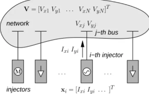
injectors j−th bus i−th injector network . . . . V= [Vx1Vy1 . . . VxNVyN]T VxjVyj IxiIyi xi= [IxiIyi. . . ]T M
Fig. 1. Power system model : network vs. injectors
(2) is a compact notation for (1) where V includes the voltage components reordered so that the vxjvariable relative to bus j occupies position 2j−1 and vyj position 2j. D is the matrix in the left-hand side of (1) reordered; it is sparse and structurally symmetric. C is a matrix with zero’s and one’s whose purpose is to extract the current components from x. Γ is a diagonal matrix with (Γ)ℓℓ = 0 if the ℓ-th equation (3) is algebraic, and (Γ)ℓℓ= 1 if it is differential.
For numerical solution, time is discretized and the differ-ential equations in (3) are algebraized using an appropriate method such as backward differentiation formulae, trapezoidal method, etc. with time step h. The resulting set of algebraic and algebraized equations can be written in compact form as:
0 = f (x, V) (4)
where the dependency on h has been omitted for simplicity. Equations (2) and (4) make up the nonlinear system to be solved at each time step by Newton method.
III. INTEGRATEDNEWTON SCHEME
Equations (4) have a structure that reflects the physical structure of the system, i.e. a set of n injectors interacting through the network only, as sketched in Fig. 1. In this paper the term injector designates any equipment connected to the network, such as a synchronous machine with its controllers, an induction motor, a dynamic or static load, a static var compensator, etc. The generic model considered hereafter is illustrated on an example in Appendix B, while the extension to components connected to two buses, such as HVDC links, TCSCs, etc. is considered in Appendix C.
The state vector x and the matrix C can be split into xi and Ci, relative to the i-th injector. Without loss of generality, it is assumed that the first two (out of ni) components of xi are Ixi and Iyi, the rectangular components of the complex current injected into the network, i.e.
xi= [IxiIyi . . .]T.
Thus, assuming that the i-th injector is connected to the j-th bus (j = 1, . . . , N ), Ci takes on the form:
Ci= [e2j−1e2j0 . . . 0 ] (5)
where e2j−1 denotes a unit vector of dimension 2N with the
Equations (2) and (4) can be rewritten as: 0 = D V− n ∑ i=1 Cixi= g(x1, . . . , xn, V) (6) 0 = fi(xi, V) i = 1, . . . , n (7)
where g is introduced for compact notation.
At a given time step the Newton method involves a sequence of linear systems (k = 1, 2, . . .): J ∆x1 ∆x2 .. . ∆xn ∆V =− f1(xk1−1, V k−1) f2(xk2−1, Vk−1) .. . fn(xkn−1, V k−1) g(xk1−1, . . . , xkn−1, Vk−1) (8)
where J is the Jacobian matrix:
J = A1 B1 A2 B2 . .. ... An Bn −C1 −C2 . . . −Cn D (9)
and incrementing the variables according to: xki = xki−1+ ∆xi i = 1, . . . , n Vk = Vk−1+ ∆V
In (9), Ai is the Jacobian of fi with respect to xi, Bi the Jacobian of fiwith respect to V and the empty entries are zero sub-matrices. Because the i-th injector involves only the Vxj and Vyj components of V, Bi is also a very sparse matrix with two nonzero columns only. All phasors are referred to axes rotating at the angular speed of the center-of-inertia, as explained in Appendix A.
Convergence is checked on the right-hand side of (8), con-taining the network and injector “mismatch” vectors. To ensure that all equations are solved within the specified tolerance, the infinite-norm (i.e. the largest component magnitude) of each mismatch vector should fall below a tolerance. Thus, the Newton iterations are stopped at iteration k if:
||g(xk 1, . . . , x k n, V k)|| ∞ < ϵg (10) ||fi(xki, V k)|| ∞ < ϵf i = 1, . . . , n (11) For the network equations, whose components are currents in per unit on the system base, the choice of ϵg is rather easy. For the injectors, on the other hand, it may be difficult to choose an appropriate ϵf value in so far as the simulation software hosts user defined models, for which the solver does not know whether a mismatch is “negligible” or not. This issue is solved by checking corrections ∆xi instead of mismatches fi, according to (i = 1, . . . , n ; j = 1, . . . , ni):
(∆xk
i)j < max(ϵa, ϵr (xki)j ) (12) Thus, the relative correction is checked against ϵr, except when (xk
i)j becomes small, in which case the absolute correction is checked against ϵa.
Clearly, the price to pay is the computation of ∆xi, which requires making at least one iteration before deciding that no further one is necessary.
IV. ACCELERATEDNEWTON SCHEME
When applied to large-scale systems, the integrated Newton scheme suffers from three drawbacks:
• when any injector undergoes a discrete change, due to a switching or a variable getting limited, Ai and Bi change and the whole Jacobian J has to be updated and factorized;
• the same holds true if convergence is slowed due to the equations of a few injectors, which triggers an update of the whole Jacobian J;
• no advantage is taken from the many injectors with “little activity” yielding negligible components in the right hand side of (8).
To tackle these issues, it is convenient to exploit the Jacobian BBD structure and decompose (8) as explained next [15].
A. Decomposing the Newton Scheme One easily obtains from (8, 9):
Ai∆xi=−fi(xki−1, V
k−1)− B
i∆V (13)
Assuming that Ai is nonsingular, ∆xi can be obtained from (13) and replaced into the last row of (8), which yields:
∑n i=1CiA−1i ( fi(xki−1, Vk−1) + Bi∆V ) + D∆V = −g(xk−1 1 , . . . , xkn−1, Vk−1) (14) Reorganizing the terms in (14) yields:
˜ D ∆V =−g(xk1−1, . . . , Vk−1)− n ∑ i=1 CiA−1i fi(xki−1, V k−1) (15) where: ˜ D = D + n ∑ i=1 CiA−1i Bi (16)
is the Schur complement [7] of diag(A1. . . An). At this point, it is convenient to define:
˜
Ci= CiA−1i (17)
and rewrite (15) and (16), respectively, as: ˜ D ∆V =−g(xk1−1, . . . , Vk−1)− n ∑ i=1 ˜ Cifi(xki−1, V k−1 ) (18) ˜ D = D + n ∑ i=1 ˜ CiBi (19)
Note that the correction ˜CiBi includes only a 2× 2 nonzero sub-matrix, centered on the diagonal of D. Hence ˜D inherits the structural symmetry and the sparsity of D.
Assuming that the Ai and ˜D matrices have been LU-factorized, and the corresponding ˜Ci matrices have been computed, the decomposed k-th Newton iteration consists of: 1) solving (18) (from the L and U factors of ˜D) to obtain
∆V and update Vk
2) solving (13) (from the L and U factors of Ai) to obtain ∆xi and update xki of each injector.
Let us emphasize that these two steps are mathematically equivalent to solving the original system (8). Step 2) can be performed concurrently and independently over the various injectors. This can be exploited in parallel processing (but is outside the scope of this paper).
The original system has been decomposed into n + 1 systems with matrices ˜D and Ai (i = 1, . . . , n) respectively. Efficient sparse solvers are available for the large, sparse and structurally symmetric matrix ˜D. A sparse solver is not justified for the Ai matrices in so far as they are relatively small and the pattern of nonzero entries change when Eqs. (3) change due to discrete events such as limits, etc.
As regards the computation of ˜Ci, (17) can be rewritten as: ATi C˜Ti = CTi
Since CTi has only two nonzero columns, so has ˜CTi. Those columns are the solutions z1 and z2of respectively:
ATiz1= e1 ATiz2= e2
where e1 (resp. e2) is a unit vector of dimension ni with the unit component in first (resp. second) position.
B. Skipping converged components
The above decomposed Newton scheme offers the possibil-ity to skip a significant amount of useless computations by:
• not updating the state vector of an injector when it has already converged;
• not updating the network voltages if the corresponding mismatches fall below the tolerance.
Assume that solving (6, 7) at a given time step requires E Newton iterations, each of them correcting first the network voltages, then the injectors states. The idea is, for injectors with low dynamic response, to perform a lower number e of iterations (e < E).
Let us recall that each injector state vector is corrected at least once, in order the convergence test (12) to be performed. Suppose that this test is passed after e iterations (e≥ 1). It can be concluded that the injector mismatch just before making the last correction, i.e. ||fi(xei−1, Ve−1)||∞ had already a negligible value. From there on, it is merely verified that the injector remains converged and, if so, (13) is not solved any longer for that injector. This verification is no longer performed using (12) (since ∆xi is not computed anymore); instead, it uses (11), where ϵf is set to ||fi(xei−1, V
e−1)|| ∞, the mismatch at the last but one iteration.
The same principle applies to the network solution: if the convergence test (10) is satisfied, Eq. (18) is not solved. C. Partially updating the Jacobian
To save computing time, it is essential to keep the Jacobian constant over several iterations and several time steps. This is commonly referred to as the “dishonest” Newton scheme.
The computational speed-up can be made even more sig-nificant using the decomposed formulation. The basic idea is to keep the Jacobians ˜D and Ai (i = 1, . . . , n) constant over as many Newton iterations and time steps as possible.
In a strict implementation of the Newton method, after updating the Jacobian Ai of the i-th injector, the ˜D matrix should be also updated and factorized owing to the CiA−1i Bi term in (16). For the same reason, when ˜D has to be updated, the Aimatrices should be computed and factorized in order to bring the latest available CiA−1i Bi terms in (16). However, extensive tests carried out by the authors on different systems have shown that the ˜D and Ai matrices can be updated independently of each other as follows:
1) when the i-th injector calls for an update of Ai, this matrix is recomputed and factorized. The ˜Ci matrix must be also recomputed since it is used in the right-hand side of (18). However, the ˜D matrix is not updated; 2) when the network calls for a Jacobian update, the Bi matrices of all injectors are updated and ˜D is computed from (19) using the available ˜Ci matrices. However, neither the Ai nor the ˜Ci matrices are updated. Regarding item 1), it is seen from (15,16) that ˜CiBi = CiA−1i Biintervenes in the ˜D matrix as the sensitivity of the current in the i-th injector to its terminal voltage. In general, it changes only slightly with operating conditions. Furthermore, it is combined with the contributions of network elements present in D; thus, the ˜D matrix is only partly affected.
V. LOCALIZEDNEWTON SCHEME
While the accelerated scheme does not affect the simulated response, the localization technique presented in this section introduces a controllable level of approximation.
A. Principle
The idea behind localization is to detect injectors with low dynamic activity (classified as latent) and replace their original models with much simpler mathematical relations. The rest of the injectors (classified as active) continue being solved without approximation. The resulting algorithm is referred to as localized Newton scheme.
Thus, an active injector is solved with the same accuracy as in a detailed simulation. The techniques detailed in Section IV-B apply to those injectors, and allow performing less iterations (13) on injectors with lower dynamic response.
For a latent injector, on the other hand, Eqs. (13) are not solved at all. Its vector fi is even not computed. Instead, it is replaced by a linear approximation between currents and voltages, as detailed in the next section.
B. Approximating the response of latent injectors
The simplified representation of a latent injector is obtained from (13) by assuming that the injector internal dynamics are negligible, i.e. fi(xki−1, Vk−1)≃ 0.
Under this approximation, (13) becomes:
Ai∆xi≃ −Bi∆V (20)
from which ∆xi is easily obtained:
Pre-multiplying (21) by Ci gives the above mentioned linear relation between current and voltage:
[∆Ixi∆Iyi0 . . . 0] T
≃ −CiA−1i Bi∆V =− ˜CiBi∆V (22) This linear formula merely involves small matrix multiplica-tions, which is much less demanding than a Newton iteration. Furthermore, the correction − ˜CiBi brought by the i-th injector to the D matrix is the same whether the injector is active or latent. Therefore, when an injector switches from active to latent or vice versa, it does not modify the ˜D matrix. The latter need not be updated, and the convergence of the Newton method is not degraded by re-using the same matrix according to the dishonest scheme.
If the i-th injector is latent, its current components Ixiand Iyiare updated according to (22) but the other components of its state vector xi are no longer updated.
C. Identifying latent injectors
Which injectors are latent and which ones are active cannot be decided a priori because it depends on the simulated disturbance. Furthermore, an injector may change from active to latent after some transients have died out, then switch back to active under the effect of the system evolving.
The linearization instant t∗i is defined as the last time the i-th injector changed from active to latent. At the beginning of the simulation, t∗i is initialized to zero for all injectors. After extensive tests, the following latency identification rules were found the most satisfactory by the authors:
1) for a “probationary” period Tp after the initial dis-turbance, all injectors are active, in order to collect information about their level of dynamic activity; 2) at the end of each time step, say at time t > Tp :
an injector switches from active to latent if its current components have not changed by more than a threshold ϵL since t = t∗i, i.e. if
|Ixi(t)− Ixi(t∗i)| < ϵL and |Iyi(t)− Iyi(t∗i)| < ϵL (23) Thus, the current is used to identify the low dynamic response of the injector, and skip it in the subsequent computations;
3) at the end of each time step, a latent injector switches from latent to active if at least one of its current components exhibits a variation larger than ϵL, i.e. if |Ik
xi(t)− Ixi(t∗i)| > ϵL or |Iyik(t)− Iyi(t∗i)| > ϵL (24) which allows latent injectors to react to new dynamics. Note that once an injector is latent, its current is computed from the linear approximation:
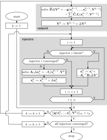
[ Ixi Iyi ] = [ Ixi(t∗) Iyi(t∗) ] − Si [ Vxi− Vxi(t∗) Vyi− Vyi(t∗) ] (25) which is merely a rewrite of (22) where the (2× 2) matrix Si contains the 4 nonzero elements of ˜CiBi. Hence, the test (24) is performed on the currents computed from (25). Therefore, the test (24) can be seen as an indirect way of monitoring the variations of the voltage at the terminal of the latent injector. Combining the localization technique with accelerated New-ton scheme of Section IV-B (for the active injectors) leads to the flowchart shown in Fig. 2.
injectors network start i:= 1 Vk:= Vk−1+ ∆Vk solve ˜D∆Vk= −g(xk−1 i , ...,x k−1 n ,Vk−1) −PC˜ifi(xk−1i ,Vk−1) k:= 1 injector i latent? injector i converged? i≤ n i:= i + 1 ||g(xk i, ...,xkn,Vk)||∞< ǫg Y all injectors converged?
stop Y k:= k + 1 k:= k + 1 N Y N N N Y Y N xk i:= xk−1i + ∆xki solve Ai∆xki = −fi(xk−1i ,V k) xk i := x ∗ i+ −A−1 i Bi∆V∗
Fig. 2. Flowchart of the accelerated and localized Newton scheme
D. Discussion
Localization enables to solve different parts of the system with different levels of accuracy depending on the level of activity of the injectors. If the threshold ϵL was set to zero, no injector would be latent; the solution accuracy would be the same throughout the whole system and unchanged with respect to the accelerated Newton scheme. When increasing ϵL, injectors with low dynamic response, likely located at some distance from the disturbance area, are considered latent. There is no risk of uncontrolled accuracy degradation in so far as only injectors with “little activity” are replaced by the linear approximation (25). Hence, in a scenario with system-wide impacts, such as the loss of interconnection tie-lines with cascading effects leading possibly to a network split, injectors previously switched to latent during the slow evolution phase will get back to active under the effect of degraded operating conditions, and accuracy will be preserved. Clearly, in such a severe case, a lower gain in computing time is to be expected, compared to the cases where the impact of the initial disturbance is limited in space.
As regards the probationary period Tp, its purpose is to give time to injectors to reveal their level of activity in response to the disturbance. Decreasing Tp activates latency earlier, and hence saves more computing time. However, too short a Tp value may lead to prematurely switching injectors to latent mode. In fact, Tp is related to the time it takes for the initial disturbance to propagate throughout the system, which
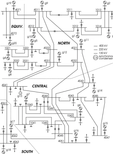
g20 g16 g17 g18 g2 g9 g1 g3 g10 g5 g4 g12 g8 g13 g14 g7 g6 g15 g11 g19 4011 4012 1011 1012 1014 1013 1022 1021 2031 cs 4046 4043 4044 4032 4031 4022 4021 4071 4072 4041 1042 1045 1041 4063 4061 1043 1044 4047 4051 4045 4062 400 kV 220 kV 130 kV synchronous condenser CS NORTH CENTRAL EQUIV. SOUTH 4042 2032
Fig. 3. Nordic32 test system
involves electromechanical oscillations mainly. Although the propagation time depends on the system size, a value of 0.5 second was found satisfactory in all systems tested by the authors, including the large one considered in Section VII.
VI. ILLUSTRATIVE EXAMPLES OF LOCALIZED SCHEME This section illustrates the performance and accuracy of the localized scheme. The results were obtained with the Nordic32 test system shown in Fig. 3 and documented in [16]. It includes 20 generators and 22 loads, i.e. 42 injectors.
A. Case N1
This case corresponds to the tripping of one circuit of the double-circuit line between buses 1013 and 1014. The simu-lation is run over 30 s, after which the system has practically regained steady-state operation. With ϵL = 0.001 pu, 23 injectors are latent for most of the simulation. This number increases to 28 for ϵL= 0.002 pu, and 36 for ϵL= 0.010 pu. All values of ϵL are in per unit on a 100-MVA base.
Generator g15, located far from the outaged line, is among them. Figure 4 shows its field voltage given by respectively the (benchmark) integrated and the localized scheme, for various values of ϵL. Note the narrow range of voltage values, indicating that the AVR of g15 responds very marginally to the disturbance. The instants at which the generator was switched to latent are easily identified by the horizontal lines, indicating
2.695 2.696 2.697 2.698 2.699 2.7 2.701 0 5 10 15 20 25 30 t (s) (pu) Integrated scheme Localized scheme with epsilonL = 0.001 Localized scheme with epsilonL = 0.002 Localized scheme with epsilonL = 0.010
Fig. 4. Case N1: field voltage of generator g15
120 140 160 180 200 0 5 10 15 20 25 30 t (s)
(MW) Localized scheme with epsilonL = 0.001Integrated scheme Localized scheme with epsilonL = 0.002 Localized scheme with epsilonL = 0.010
190 192 194 196 198 200 1.5 2 2.5 3 3.5 t (s)
Fig. 5. Case N1: active power flow in remaining circuit of line 1013-1014
that the generator states (including its field voltage) are no longer updated. The larger ϵL, the sooner the switching.
The power flow in the parallel, remaining circuit is shown in Fig. 5, with a zoomed view on the first two seconds following the probationary period. The curves of the four algorithms are indistinguishable. No loss of accuracy results from localization.
B. Case N2
This more severe case involves the outage of the line between buses 4043 and 4047. After electromechanical oscil-lations have died out, the system responds with two Load Tap Changers (LTC) acting at t = 38 and t = 46 s, respectively, to restore distribution voltages within their dead-bands.
Figure 6 shows the evolution over 20 s of the active power of generator g15, located next to the tripped line and, hence, significantly impacted by the disturbance. The evolutions computed with the localized scheme, using ϵL = 0.001 or 0.002 pu, are essentially the same as that of the integrated scheme and, therefore, they are not shown. For ϵL= 0.010 pu, the average (resp. largest) absolute difference between the exact and localized responses is only 0.1 % (resp. 0.7 %) of the initial active power.
950 1000 1050 1100 1150 0 5 10 15 20 t (s) (MW) Integrated scheme Localized scheme with epsilonL = 0.010
Fig. 6. Case N2: active power produced by generator g15
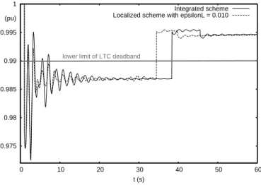
0.975 0.98 0.985 0.99 0.995 1 0 10 20 30 40 50 60 t (s) (pu) Integrated scheme Localized scheme with epsilonL = 0.010
lower limit of LTC deadband
Fig. 7. Case N2: distribution voltage controlled by an LTC
The effects of localization may be more noticeable on discrete events, such as tap changes. Figure 7 shows the voltage at the distribution bus controlled by one of the above mentioned LTCs. Before the first tap change, the maximum discrepancy between the localized (with ϵL = 0.010 pu) and reference evolutions is 0.004 pu, to be compared to the LTC voltage dead-band of 0.020 pu. In the reference simulation, voltage swings reset the LTC timer four times, before the voltage eventually leaves its dead-band. With the localized scheme, the distribution voltage leaves its dead-band three seconds earlier, which causes the tap change to be shifted by the same time. Such a time shift (to be compared to the 20 s delay on the first tap change) is not significant as the error introduced during the three seconds is 0.01 pu only. Furthermore, the voltage eventually reaches the same value.
VII. SIMULATION RESULTS ON A LARGE-SCALE SYSTEM
A. PEGASE test system
Within the context of the PEGASE project [17], a test sys-tem inspired of the pan-European transmission grid has been set up, with the objective of testing the proposed approaches on a large-scale model. The main features of the model are:
0 50 100 150 200 t (s)
Fig. 8. Discrete event occurrence in Case C3
• 15226 buses and 21765 branches;
• 3483 synchronous machines with generic models of their excitation systems, AVRs, OELs, turbines and speed governors;
• 7211 dynamic loads. Some of them are equivalents of dis-tribution systems with step-down transformers, medium-voltage feeders and induction motor loads;
• 2945 LTCs represented as discrete devices.
This leads to a model with 146239 states. Among these, 72293 are differential and 73946 algebraic (out of which 30452 are Vx, Vy voltage components), which yields an average of 22 state variables per power plant and 5 per dynamic load. The size of matrices Ai ranges between 4 and 29. More information and results from this system can be found in [18]. B. Algorithms and scenarios
The results of the following three algorithms are presented: I : Integrated Newton scheme (8, 9) in which J is updated after a discrete change in any injector or after 3 successive iterations in the same time step (this offers a good compromise between the burden of updating the factors and the burden of performing too many iterations); A : Accelerated Newton scheme with (network and injector)
Jacobians updated independently and infrequently (see Section IV-C) and solution of converged injectors skipped (see Section IV-B);
L : same as A, with response localized (see Section V). All values of ϵL are in per unit on a 100-MVA base. One short- and two long-term cases are reported as follows: C1 : simulation over 20 s of a double-circuit line outage; C2 : simulation over 240 s of two double-circuit line outages; C3 : simulation over 240 s of a bus-bar fault cleared in 0.1 s
by opening the lines involved in Case C2.
The differential equations were algebraized using the Back-ward Differentiation Formula of order 2:
x(tj) = 4 3x(tj− h) − 1 3x(tj− 2h) + 2h 3 x(t˙ j) (26) The step size h was set to 0.01 s in the half second after the initial disturbance, then increased to 0.05 s. Results for various step sizes are presented in Section VI.D.
The sequence of discrete events experienced in case C3 is shown in Fig. 8, where the spikes indicate variables hitting or leaving their limits, timers that start counting time, or LTC moves (between t ≃ 27 and 236 s, to restore the controlled voltages within their dead-bands). As many as 1988 events take place during this 4-minute simulation. The limits on variables are treated as explained in [19], while LTC changes are enforced at the first discrete time after they have been identified to take place.
0 0.001 0.002 0.003 0.004 0.005 0 0.002 0.004 0.006 0.008 0.01 0.012 0.014 0.016 0.018 0.02 epsilonL (pu) (pu) Case C1 Case C2 Case C3
Fig. 9. Worst average voltage error µ for various ϵLvalues
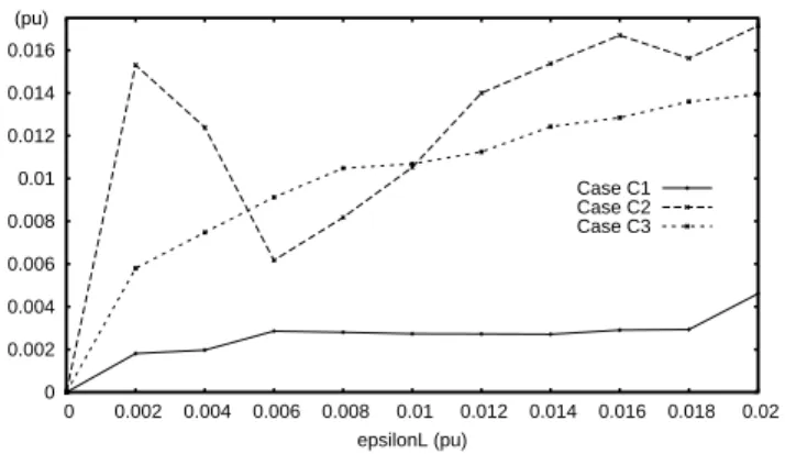
0 0.002 0.004 0.006 0.008 0.01 0.012 0.014 0.016 0 0.002 0.004 0.006 0.008 0.01 0.012 0.014 0.016 0.018 0.02 epsilonL (pu) (pu) Case C1 Case C2 Case C3
Fig. 10. Worst maximum absolute voltage error ν for various ϵLvalues
C. Implementation aspects
All results were obtained with the RAMSES software devel-oped at the Univ. of Li`ege. It is written in FORTRAN 2003. This language, popular in High Performance Computing, pro-vides numerous optimized numerical (intrinsic) procedures, is inter-operable with C, allows reusing legacy FORTRAN code, and facilitates parallel programming.
The partial derivatives relative to network and synchronous machine equations are computed analytically, while those relative to the machine controllers as well as the other injectors are evaluated by finite differences.
In Schemes A and L, the injector systems (13) are factorized and solved with the DGETR BLAS routines for dense matrices, while the sparse solver ma41 from the Harwell library [20] is used to deal with the network system (15, 16). The same sparse solver is used for the whole Jacobian in Scheme I.
D. Accuracy and choice of ϵL
As already mentioned, scheme A yields the same accuracy as scheme I, while for scheme L, choosing ϵLinvolves a trade-off between accuracy and computational effort.
It is advisable to select ϵL once for all for a given system, based on the analysis of a set of representative disturbances. There is a good deal of engineering judgment in this choice, as for other typical settings of a solver (such as ϵg, ϵf, ϵa and ϵr, see Section III). However, it can be guided by a simple quantitative analysis of the type shown hereafter.
The impact of ϵL on accuracy has been assessed on a subset of significant state variables; results are presented for bus voltage magnitudes. Let Vi(k, ϵL) denote the voltage magnitude of the i-th bus (i = 1, . . . , N ), at the k-th discrete time (k = 1, . . . , ns) of a scheme-L simulation with latency tolerance ϵL. The following metrics have been computed:
µ(ϵL) = max i=1,...,N 1 ns ns ∑ k=1 ( Vi(k, ϵL)− Vi(k, 0) ) (27) ν(ϵL) = max i=1,...,Nk=1,...,nmax s |Vi(k, ϵL)− Vi(k, 0)| (28) where Vi(k, 0) is the (reference) voltage value obtained with-out latency approximation.
µ is the worst average voltage error. Its variation with ϵL is shown in Fig. 9, for the three disturbances mentioned in Section VII.B. Note that from one point to another, the maximum value in (27) may take place on different buses (yet close to the disturbance location). The curves suggest that it is appropriate to set ϵL to 0.01 pu, since some degradation is observed for higher values in Case C3.
ν is the worst maximum absolute voltage error. Its variation with ϵL is shown in Fig. 10. For ϵL = 0.01 pu, the largest voltage error at any bus and any time is around 1 %. The peak observed for ϵL = 0.002 pu in Case C3 is due to one voltage settling at a slightly different value under LTC dead-band effects, as described in Section VI.B.
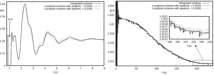
By way of illustration, the short- and long-term evolutions of the voltage at the faulted bus in case C3 are shown in Fig. 11. The results of Scheme A are not shown, as they are indistinguishable from those of Scheme I. Two values of ϵL are considered. The good accuracy obtained with ϵL = 0.01 pu confirms the above analysis.
E. Computational effort
Table I details the computing times obtained with the various schemes in the three cases. CPU times were measured on a standard laptop with the following characteristics: Intel Core i7-2630QM CPU, 2.9 GHz, 8 GB RAM, running under Ubuntu Linux 11.04. The CPU times were obtained by code profiling using Intel VTune Amplifier XE, and do not take into account data reading and loading (which is the same for all three algorithms). The table also shows the number of major operations performed. The results relative to injectors are average values per injector.
A comparison of Schemes A and I shows that the highest gain is at the factorization level, since Scheme A allows updating only small sub-matrices of the whole Jacobian, while Scheme I performs full Jacobian updates. A significant gain is also obtained by skipping solutions of converged injectors. A slightly larger time is spent in injector function evaluations. Compared to Scheme I, Scheme A offers a speed-up ranging from 1.9 to 2.7, at no cost regarding accuracy.
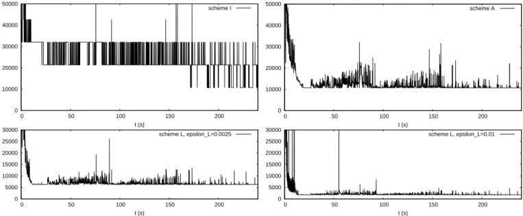
Figure 12 shows the number of injector solutions computed at each time step. With Scheme I (upper left plot), solutions are computed for all injectors at each Newton iteration. Thus, with n = 10694 injectors, the plot shows values in multiples of n: most of time, 1,2 or 3 Newton iterations are enough. The
1 1.01 1.02 1.03 1.04 1.05 1 2 3 4 5 6 7 8 9 t (s) (pu) Integrated scheme Localized scheme with epsilonL = 0.0025 Localized scheme with epsilonL = 0.0100
fault 1.012 1.014 1.016 1.018 1.02 1.022 1.024 0 50 100 150 200 t (s) (pu) Integrated scheme Localized scheme with epsilonL = 0.0025 Localized scheme with epsilonL = 0.0100
1.0112 1.0113 1.0114 1.0115 1.0116 1.0117 1.0118 1.0119 1.012 1.0121 190 200 210 220 230 240 t (s)
Fig. 11. Case C3: short-term (left plot) and long-term (right plot) evolution of voltage at faulted bus TABLE I
CPUTIMES(IN SECONDS)AND NUMBER OF MAJOR OPERATIONS(FIGURES MARKED WITH A⋆ARE AVERAGES PER INJECTOR)
Scheme I Scheme A Scheme L
ϵL= 0.001 ϵL= 0.0025 ϵL= 0.01
time nb. op. time nb. op. time nb. op. time nb. op. time nb. op.
CASE C1
factorizing J 57.51 446 factorizing ˜D 0.69 25 0.97 32 0.76 26 0.71 25
solving for [∆V ∆x]T 11.19 1393 solving for ∆V 0.82 1031 1.06 1158 1.06 1009 0.69 844
evaluating [g f ]T 13.11 1891 evaluating g 1.97 2326 1.75 2320 2.07 2429 1.81 2012 factorizing Ai 2.84 26⋆ 1.34 16⋆ 1.23 15⋆ 1.04 13⋆ solving for ∆xi 6.51 792⋆ 5.26 594⋆ 4.66 478⋆ 2.43 255⋆ evaluating fi 14.75 2321⋆ 12.67 1805⋆ 10.28 1443⋆ 5.12 719⋆ total 90.29 total 32.81 27.49 24.45 15.10 CASE C2 factorizing J 207.58 1597 factorizing ˜D 0.75 27 1.05 36 0.96 32 0.79 28
solving for [∆V ∆x]T 90.00 11106 solving for ∆V 7.42 8514 7.39 8620 8.25 8476 8.11 8167
evaluating [g f ]T 111.86 15988 evaluating g 14.04 17160 14.92 18104 14.66 18310 13.46 17725 factorizing Ai 2.51 22⋆ 1.13 14⋆ 1.25 16⋆ 0.98 13⋆ solving for ∆xi 41.53 5634⋆ 33.07 3521⋆ 20.73 2089⋆ 7.57 718⋆ evaluating fi 117.25 19044⋆ 88.07 12212⋆ 54.76 7192⋆ 19.61 2305⋆ total 470.00 total 220.21 181.35 132.41 75.34 CASE C3 factorizing J 179.40 1374 factorizing ˜D 0.93 32 0.99 34 1.03 34 1.14 35
solving for [∆V ∆x]T 88.93 10975 solving for ∆V 8.19 8556 7.87 8547 7.83 8362 7.65 8368
evaluating [g f ]T 111.34 15946 evaluating g 13.91 17020 13.94 17052 14.32 17337 14.53 18303
factorizing Ai 4.49 40⋆ 3.26 35⋆ 2.56 27⋆ 3.39 42⋆
solving for ∆xi 47.35 5757⋆ 38.74 4744⋆ 29.69 3429⋆ 13.69 1290⋆
evaluating fi 119.44 19285⋆ 106.06 15991⋆ 83.23 11572⋆ 34.00 4278⋆
total 438.21 total 232.56 209.18 174.35 102.48
upper right plot in Fig. 12 shows the corresponding result with Scheme A. The lower bound is n, since at least one iteration per injector is performed at each step. As in Scheme I, some of the injectors require more than 3 iterations; on the other hand, a vast majority of injectors is already solved (up to the same tolerance) with just one iteration.
A small subset of injectors require more iterations and are also responsible for the much higher number of Jacobian factorizations in Scheme I. Indeed, in scheme A, the slow convergence of one injector leads to updating its own Jacobian only, while in scheme I it slows down the convergence of the whole system, forcing to perform many full Jacobian updates. With the use of localization (scheme L), as expected, the
computational effort is reduced with the increase of ϵL. The tables show that the highest gain stems from the evaluations and the solutions of the injectors: indeed, with respect to scheme A, several injectors are latent for some part of the simulation. The decrease in number of injector factorizations is milder, as it is the most “active” injectors which need to be factorized the most, in both schemes, and are thus not affected by latency. On the network, on the other hand, the gain is imperceptible, if not negative in some cases: indeed, the network cannot be latent, while a slight degradation is possible due to the approximations brought by the latent injectors. The speed-up brought by Scheme L compared to Scheme I ranges from 2.1 to 6.2, for a negligible decrease in accuracy.
0 10000 20000 30000 40000 50000 0 50 100 150 200 t (s) scheme I 0 10000 20000 30000 40000 50000 0 50 100 150 200 t (s) scheme A 0 5000 10000 15000 20000 25000 30000 0 50 100 150 200 t (s) scheme L, epsilon_L=0.0025 0 5000 10000 15000 20000 25000 30000 0 50 100 150 200 t (s) scheme L, epsilon_L=0.01
Fig. 12. Case C3: number of injector solutions at each time step with Schemes I, A and L (y-axis limited to respectively 50,000 and 30,000, for legibility)
The lower two plots in Fig. 12, relative to two values of ϵL confirm the dramatic decrease in number of solutions brought by Scheme L. The lower bound corresponds to the number of injectors which cannot become latent because they experience a large variation of the current with respect to their linearization point, which for injectors with strong dynamic activity was taken at t∗= 0. This lower bound is around 2000 for ϵL= 0.01 pu and 7000 for ϵL= 0.0025 pu.
Varying the step size is another well-known way of saving computing time. Automatic step size adjustment based on es-timates of the local truncation error is a proven technique [21]. The results reported so far relate to simulations with a constant step size (except for a short interval after the disturbance). The reason is that, the system response being slightly affected by localization, Scheme L would yield different time steps with respect to the other two schemes. This would make it more difficult to assess the gain brought by localization. However, results obtained when running the proposed algorithms with different values of h are reported hereafter.
The variation of the CPU times with h is shown in Fig. 13, relative to case C3 and ϵL= 0.01 pu. The range of h values is reasonable considering that the average time between discrete events is 0.12 s (1988 events in 240 s: see Fig. 8); the average value of h could not be much larger with an accurate variable-step size solver, unless tap changes are delayed in order more of them to take place at the same time steps. That solver would also spend time in identifying the discrete event times and updating Jacobians due to changes in h. The shown CPU times have been normalized by dividing them by the time taken by Scheme I with h = 0.01 s. The computing times decrease when h increases, as expected.
The figure also shows the speed-up, defined as the CPU time of Scheme I divided by that of Scheme A (resp. L), for a given value of h. For Scheme A, the best speed-up is 2.7. For Scheme L it is 5.3, but it was found to be 7.9 in Case C2. These results allows concluding that variable-step size solvers would also benefit from the proposed solution schemes.
0 0.2 0.4 0.6 0.8 1 0.02 0.04 0.06 0.08 0.1 0.12 0.14 1 1.5 2 2.5 3 3.5 4 4.5 5 5.5 h (s)
normalized CPU time speed-up
normalized CPU time: Scheme I normalized CPU time: Scheme A normalized CPU time: Scheme L speedup of Scheme A wrt I speedup of Scheme L wrt I
Fig. 13. Case C3: normalized CPU times and speed-ups of various schemes
VIII. CONCLUSION
Methods to speed up time simulations of large-scale power systems have been proposed. Tests performed on a large-scale system (around 146, 000 differential-algebraic states) have confirmed the possibility to obtain the expected speed-up. The proposed techniques exploit the bordered block-diagonal structure of the Jacobian involved at each Newton iteration. An accelerated scheme has been proposed to mini-mize the number of partial Jacobian updates and factorizations, and perform less iterations on components with lower dynamic response. It brings a speed-up ranging between 2 and 3, for the same accuracy as an integrated Newton method.
Further speed-ups have been obtained by localizing the system response, i.e. by exploiting the fact that, in a large-scale system, some components do not participate much in the dynamic response. After a probationary period Tp, latent components are not solved, but replaced by a static linear model relating injected current to bus voltage. The degradation of accuracy is bounded and easily controlled by the latency tolerance ϵL, which can be interpreted as the current variation
which is considered negligible. It is recommended to adjust ϵL once for all for a given system. Some quantitative analysis guidelines have been presented.
The accelerated and localized scheme offers a speed-up ranging between 4 and 8, with respect to an integrated Newton method, while still providing reasonably accurate responses.
Within the context of the PEGASE project, the algorithms have been implemented in a dynamic simulation prototype derived from EUROSTAG and a dispatch training simulator prototype based on FAST [22].
ACKNOWLEDGEMENT
The contributions (after PEGASE project) of Petros Aris-tidou, Ph.D. student at the Univ. of Li`ege, are gratefully acknowledged.
APPENDIXA
REFERENCE FRAME FOR PHASORS
All phasors must be projected on the same reference (x, y) axes but the choice of the latter is free.
Axes rotating at nominal angular frequency 2πfo are not suited for long-term simulations. Indeed, consider for instance the case where the system settles in steady state with frequency f ̸= fo. Since all phasors rotate at speed 2π(f − fo) with respect to the axes, their projections of the (x, y) axes oscillate at frequency|f − fo|. Thus, although the system is in steady state, its simulation requires quite some computational effort. This problem disappears when taking (x, y) axes rotating at the speed of the Center-Of-Inertia (COI):
ωcoi= ∑ iMiωi ∑ iMi (29) where ωi is the rotor speed of the i-th synchronous machine, and Mi its inertia coefficient. With that reference, the model of each machine includes the equation:
˙δi= ωi− ωcoi i = 1, . . . , m (30) One possibility is to handle ωcoi as an additional algebraic variable, and add (29) to the original set of equations. How-ever, that equation and the presence of ωcoi in all equations (30) hinders the decomposition defined in Section IV.A.
This drawback is avoided with the reference frame proposed in [23]. It involves (x, y) axes rotating with speed at time t equal to ωcoi(t− h), i.e. the speed of the COI at the previous time step. By so doing, ωcoiin (30) is replaced by ωcoi(t−h), which is a constant, no longer a variable. Equation (29) is not handled together with the other equations; it is used to update ωcoi at the end of each time step, for use at the next one. The BBD structure of the Jacobian is preserved while retaining the advantage of the COI reference.
In case of network split, one COI reference is used per connected sub-system. As regards localization, when a syn-chronous machine gets latent, it is still accounted in (29) but with ωi at time t set equal to ωcoi(t− h).
APPENDIXB
EXAMPLE OF INJECTOR MODEL
The injector formulation used throughout the paper is illus-trated on the single-cage induction motor model.
Using Park transformation, the three-phase stator and rotor windings are replaced by (d, q) windings attached to the (x, y) axes defined in the previous section [1].
Neglecting transformer voltages, the stator equations are: 0 = Vy− RsIy− ωcoi(Lss− L2 sr Lrr )Ix− ωcoi Lsr Lrr ψqr (31a) 0 = Vx− RsIx+ ωcoi(Lss− L2 sr Lrr )Iy− ωcoi Lsr Lrr ψdr (31b) where Rs is the stator resistance, Lss the stator self-inductance, Lrr the rotor self-inductance, Lsr the mutual inductance between stator and rotor, ψdr (resp. ψqr) the flux linkage in the d-axis (resp. q-axis) rotor winding. The voltage and current components have been defined in Section II.
The rotor flux linkages evolve according to: ˙ ψdr=− Rr Lrr ψdr+ Rr Lsr Lrr Iy− (ωcoi− ω)ψqr (32a) ˙ ψqr=− Rr Lrr ψqr+ Rr Lsr Lrr Ix− (ωcoi− ω)ψdr (32b) where Rr is the rotor resistance and ω is the rotor speed.
Finally, the rotor motion equation is written as: ˙ ω = 1 2H ( Lsr Lrr (ψqrIy− ψdrIx)− Tm(ω) ) (33) where H is the inertia constant and Tmthe mechanical torque, varying with ω according to the type of mechanical load.
The state vector xi = [Ix Iy ψdr ψqr ω]T involves alge-braic and differential states according to Γ = diag (0 0 1 1 1).
The following Jacobian sub-matrices are easily derived:
Ai = −X′ s −Rs 0 −ωcoik 0 −Rs Xs′ −ωcoik ω 0 0 kRr − Rr Lrr ω ψqr kRr 0 ω − Rr Lrr ψdr −kψdr 2H kψqr 2H − kix 2H kiy 2H 1 2H dTm dω where Xs′ = ωcoi(Lss− L2 sr Lrr ) and k = Lsr Lrr , Bi= 0 0 0 1 0 0 0 0 1 0 0 0 0 . . . 0 0 0 0 . . . 0 0 0 0 0 0 0 0 0 0 0 0 0
where the first (resp. second) nonzero column refers to the vx (resp. vy) component of the complex voltage at the bus where the motor is connected. In an N -bus system, Ci in (5) is a 2N × 5 matrix, Bi is a 5× 2N matrix, and CiA−1i Bi is a 2N× 2N matrix with only four nonzero terms.
APPENDIXC EXTENSION TO TWO-PORTS
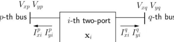
The single-port structure of injectors is not suited to model two-port devices controlling the currents injected at two buses, such as HVDC links, TCSCs and other FACTS devices. To deal with the latter, the derivations of this paper are easily extended to the two-port component sketched in Fig. 14.
i-th two-port
p-th bus q-th bus
VxpVyp VxqVyq
Ixip Iyip xi Ixiq Iyiq
Fig. 14. Variables involves in a two-port component
The two-port state vector includes four current components (instead of two): xi= [Ixip I p yiI q xiI q yi . . .] T.
The corresponding Bi matrix has four nonzero rows while Cihas four nonzero columns. The Schur complement compu-tation is unchanged. It involves a 2N× 2N matrix CiA−1i Bi with 16 nonzero terms, located in four 2 × 2 blocks, two diagonal and two off-diagonal, respectively. The structural symmetry of D is preserved.
A two-port switches to latent when both currents satisfy (23), and to active when at least one current satisfies (24).
REFERENCES
[1] P. Kundur, Power system stability and control. The EPRI power system engineering series, McGraw-Hill, 1994.
[2] J. Machowski, J. W. Bialek, and J. R. Bumby, Power System Dynamics
and Stability. John Wiley, 1997.
[3] CIGRE Working group C4.601, Review of On-line Dynamic Security
Assessment Tools and Techniques. Technical Brochure 325, CIGRE,
2007.
[4] K. Strunz and E. Carlson, “Nested Fast and Simultaneous Solution for Time Domain Simulation of Integrative Power Electric and Electronic Systems,” IEEE Trans. on Power Delivery, vol. 22, pp. 277–287, Jan. 2007.
[5] F. Pruvost, T. Cadeau, P. Laurent-Gengoux, F. Magoules, F.-X. Bouchez, and B. Haut, “Numerical accelerations for power systems transient sta-bility simulations,” in Proc. 17th Power System Computation Conference
(PSCC), pp. 1–8, Aug. 2011.
[6] S. K. Khaitan, J. D. McCalley, and Q. Chen, “Multifrontal Solver for Online Power System Time-Domain Simulation,” IEEE Trans. Power
Syst., vol. 23, pp. 1727–1737, Nov. 2008.
[7] F. Zhang, The Schur complement and its applications. Numerical methods and algorithms, Springer Science, 2005.
[8] G. D. Hachtel and A. L. Sangiovanni-Vincentelli, “A survey of third-generation simulation techniques,” Proceedings of the IEEE, vol. 69, pp. 1264–1280, Oct. 1981.
[9] Power System Dynamic Analysis Phase I. EPRI EL-484 Project 670-1, Final report, EPRI, 1977.
[10] J. Fong and C. Pottle, “Parallel Processing of Power System Analysis Problems Via Simple Parallel Microcomputer Structures,” IEEE Trans.
Power Apparatus and Systems, vol. PAS-97, pp. 1834–1841, Sept. 1978.
[11] Extended Transient-Midterm Stability Program: Version 3.0. EPRI TR-102004 Project 1208-09, Final report, EPRI, 1993.
[12] M. L. Crow and J. G. Chen, “The multirate method for simulation of power system dynamics,” IEEE Trans. Power Syst., vol. 9, pp. 1684– 1690, Aug. 1994.
[13] V. Brandwajn, “Localization Concepts in (In)-Security Analysis,” in
Proc. 1993 Athens Power Tech Conf., vol. 1, pp. 10–15, Sept. 1993.
[14] J. Ogrodzki, Circuit simulation methods and algorithms. Electronic engineering systems series, CRC Press, 1994.
[15] D. Fabozzi and T. Van Cutsem, “Localization and latency concepts applied to time simulation of large power systems,” in Proc. 2010 Bulk
Power System Dynamics and Control - VIII IREP Symp., Aug. 2010.
[16] T. Van Cutsem, Description, Modeling and Simulation Results of a Test
System for Voltage Stability Analysis. Internal report, University of Li`ege, http://hdl.handle.net/2268/141234, 2013.
[17] PEGASE project. http://www.fp7-pegase.eu, accessed July 2012. [18] D. Fabozzi, Decomposition, Localization and Time-Averaging
Ap-proaches in Large-Scale Power System Dynamic Simulation. PhD thesis,
University of Li`ege, http://hdl.handle.net/2268/126720, 2012. [19] D. Fabozzi, A. S. Chieh, P. Panciatici, and T. Van Cutsem, “On simplified
handling of state events in time-domain simulation,” in Proc. 17th Power
System Computation Conference (PSCC), Aug. 2011.
[20] HSL. A collection of Fortran codes for large scale scientific computation. http://www.hsl.rl.ac.uk, accessed May 2012.
[21] M. Stubbe, A. Bihain, J. Deuse, and J. C. Baader, “STAG-a new unified software program for the study of the dynamic behaviour of electrical power systems,” IEEE Trans. Power Syst., vol. 4, pp. 129–138, Feb. 1989.
[22] EUROSTAG and FAST. http://www.eurostag.be, accessed July 2012. [23] D. Fabozzi and T. Van Cutsem, “On angle references in long-term
time-domain simulations,” IEEE Trans. Power Syst., vol. 26, pp. 483–484, Feb. 2011.
Davide Fabozzi(S’09) received the B.Eng. and M.Eng. degrees in Electrical Engineering from the Univ. of Pavia, Italy, in 2005 and 2007, respectively. In 2007 he joined the Univ. of Li`ege, where he received the Ph.D. degree in 2012. Presently, he is a Marie Curie Experienced Researcher Fellow at Imperial College London, UK. His research interest include simulation of differential-algebraic and hybrid systems, power system dynamics and frequency control.
Angela S. Chieh (M’11) graduated from Ecole Polytechnique, France, in 2008. In the same year, she received the Engineering MSc degree from Telecom ParisTech. She joined the “System Expertise” Dept. of RTE in 2009, where she is working on research and development of power system analysis tools, such as EUROSTAG, and contributing to projects such as PEGASE.
Bertrand Hautgraduated in Applied Mathematics Engineering in 2003 and obtained his Ph.D. in 2007 from the Catholic Univ. of Louvain, Belgium. Since then he has been with the power consulting Dept. of Tractebel Engineering, currently on time-domain simulation and small-signal analysis.
Thierry Van Cutsem(F’05) graduated in Electrical-Mechanical Engineering from the Univ. of Li`ege, Belgium, where he obtained the Ph.D. degree and he is now adjunct professor. Since 1980, he has been with the Fund for Scientific Research (FNRS), of which he is now a Research Director. His research interests are in power system dynamics, security, monitoring, control and simulation, in particular voltage stability and security. He is currently Chair of the IEEE PES Power System Dynamic Performance Committee.