Any correspondence concerning this service should be sent to the repository administrator:
[email protected]
To link to this article:
DOI:10.1016/j.jclepro.2011.09.011
http://dx.doi.org/10.1016/j.jclepro.2011.09.011
This is an author-deposited version published in:
http://oatao.univ-toulouse.fr/
Eprints ID: 6537
To cite this version:
Boix, Marianne and Montastruc, Ludovic and Pibouleau, Luc and
Azzaro-Pantel, Catherine and Domenech, Serge Industrial water management by
multiobjective optimization: from individual to collective solution through
eco-industrial parks. (2012) Journal of Cleaner Production, vol. 22 (n° 1). pp. 85-97.
ISSN 0959-6526
O
pen
A
rchive
T
oulouse
A
rchive
O
uverte (
OATAO
)
OATAO is an open access repository that collects the work of Toulouse researchers and
makes it freely available over the web where possible.
Industrial water management by multiobjective optimization: from individual
to collective solution through eco-industrial parks
Marianne Boix, Ludovic Montastruc, Luc Pibouleau
*, Catherine Azzaro-Pantel, Serge Domenech
Laboratoire de Génie Chimique (LGC), Centre National de la Recherche Scientifique (CNRS), Institut National Polytechnique de Toulouse (INPT), Université de Toulouse, 4, Allée Emile Monso, BP 84234, 31432 Toulouse, France
Keywords: Water network Multiobjective optimization MILP Eco-industrial park
a b s t r a c t
Industrial water networks are designed in the first part by a multiobjective optimization strategy, where fresh water, regenerated water flow rates as well as the number of network connections (integer vari-ables) are minimized. The problem is formulated as a Mixed-Integer Linear Programming problem (MILP) and solved by the ε-constraint method. The linearization of the problem is based on the necessary conditions of optimality defined by Savelski and Bagajewicz (2000). The approach is validated on a published example involving only one contaminant. In the second part the MILP strategy is imple-mented for designing an Eco-Industrial Park (EIP) involving three companies. Three scenarios are considered: EIP without regeneration unit, EIP where each company owns its regeneration unit and EIP where the three companies share regeneration unit(s). Three possible regeneration units can be chosen, and the MILP is solved under two kinds of conditions: limited or unlimited number of connections, same or different gains for each company. All these cases are compared according to the global equivalent cost expressed in fresh water and taking also into account the network complexity through the number of connections. The best EIP solution for the three companies can be determined.
1. Introduction
During the last decades, many developed countries have increased their investment in environmental research and devel-opment due to an increasing depletion of natural resources such as fresh water for instance (UNESCO, 2009). With the increasing interest for global environment preservation, the unlimited resources paradigm became little by little obsolete. In 2008, the global needs in fresh water were estimated to be 4000 km3 (UNESCO, 2009), where 20% were used by industry and have been globally increased by a factor of four during the last 50 years (Oecd, 2008). The environmental impact induced by the process industry is linked both to the high volumes involved and to the diversity of toxic products generated along the processing chain. Consequently, a real need to define optimized water networks so as to reduce the impact of contaminants on the environment, has recently emerged.
Although the world concern of sustainable development gave birth to a lot of works during the last decades, the concept of Industry linked to Ecology is quite much older. Indeed, since the beginning of the twentieth century, scientists are worried about designing clean industries. Several studies stated the recycling of by-products of an industry by another one (Simmonds, 1862; Conover, 1918). These studies did not introduce any official term on what they dealt for. “Industrial Ecology” really appeared (Hoffman, 1971) in the 1970’s and Japanese and Belgian studies went deeper in this topic (Watanabe, 1972; Gussow and Meyers, 1970). However, Frosch and Gallapoulos (1989) popularized this term twenty years ago from the idea that we should use the analogy of natural systems as an aid in understanding how to design sustainable industrial systems. As they indicate the ideal ecosystem, in which the use of energy and materials is optimized, wastes and pollution are minimized and there is an economically viable role for every product of a manufacturing process, will not be attained soon. It was true in 1989, and it is always true today.
Industrial Ecology has been defined by Allenby (2006)as “a systems-based, multidisciplinary discourse that seeks to under-stand emergent behaviour of complex integrated human/natural systems”. In most of the researches in Industrial Ecology the common guideline is that natural systems do not have waste in
* Corresponding author. Tel.: þ335 34 32 36 58; fax: þ335 34 32 37 00. E-mail addresses: [email protected] (M. Boix), ludovic.montastruc@ ensiacet.fr (L. Montastruc), [email protected] (L. Pibouleau),
[email protected](C. Azzaro-Pantel),[email protected]
(S. Domenech).
them, so our systems should be modeled from natural ones if we want them to be sustainable.
Without falling into the trap of abstruse ecological discourses, many difficult societal and/or industrial problems appear under the generic term of Industrial Ecology. Building a sustainable industry is slightly linked to the term Industrial Symbiosis. According to Chertow (2000), an industrial symbiosis engages “separate indus-tries in a collective approach to competitive advantage involving physical exchange of materials, energy, water and by-products”. A primordial feature of an industrial symbiosis is the collaboration offered by the geographic proximity of the several companies. Most widespread manifestations of an industrial symbiosis are Eco-Industrial Parks. The term “eco-industrial park” is the subject of many debates due to its definition, difficult to formulate rigorously. However, a definition commonly adopted is “an industrial system of planned materials and energy exchanges that seeks to minimize energy and raw materials use, minimize waste, and build sustain-able economic, ecological and social relationships” (PCSD, 1996; Alexander et al., 2000). This definition was later reported byCôté and Cohen-Rosenthal (1998). Obviously, a basic condition for an EIP to be economically viable is to demonstrate that the sum of benefits achieved by working as collective is higher than working as a stand-alone facility.
There is some amount of uncertainty in this type of optimization model. For instance, the mass loads of contaminants for water-using processes or any other parameter that may changes during the operation process. Although some studies (Sahinidis, 2004; Karuppiah and Grossmann, 2008) have incorporated these uncer-tainties to design industrial water networks, the objectives of this study.
The first part of this paper aims at defining a general method-ology by taking into account only the single contaminant case for the Design of Water Networks (DWN). The generic problem is formulated under a MILP form with integer variables related to the connections into the network. The biobjective optimization of the fresh water flow rate at the network entrance and the water flow
rate at regeneration unit inlets, parameterized by the number of connections, is carried out according to a lexicographic procedure. The approach, validated on a published example involving ten processes and one regeneration unit, is extended in the second part to eco-industrial parks (EIP). The last part deals with several EIP configurations in order to evaluate the feasibility of each solution. 2. Previous works
Historically, the design of water network (DWN) was carried out not for EIP purposes, but for a stand-alone company by means of graphical methodologies (Dunn and Wenzel, 2001; Jacob et al., 2002; Linnhoff and Vredeveld, 1984; Manan et al., 2006; Wan Alwi, 2008), mathematical programming (Bagajewicz and Savelski, 2001; Feng et al., 2008; Huang et al., 1999) and synthesis of mass exchange networks (El-Halwagi, 1997; Hallale and Fraser, 2000; Shafiei et al., 2004). Designing water networks refers to allocate the streams of the networks between several units while respecting constraints and satisfying objectives. Water allo-cation problems (WAP) were widely studied during the last decades due to the growing interest for sustainable development in industries (de Faria and de Souza, 2009; Kumaraprasad and Muthukumar, 2009; Klemes et al., 2010; Poplewski et al., 2010). Linear formulations implemented for maximizing water regener-ation and reuse into industrial processes has been first developed in a lot of previous works (Bagajewicz and Savelski, 2001; El-Halwagi, 1997; El-Halwagi et al., 2004; Wang and Smith, 1994). These techniques are limited to single contaminant networks (Gomes et al., 2007), which are the main subject of the present study Another strategy has already been adopted regarding the resolu-tion of WAP, it consists in multiobjective optimizaresolu-tion using genetic algorithm (Lavric et al., 2005). Nonlinear strategies based on the relaxation of the bilinear terms involved in the balance equations are presented in the works of Quesada and Grossmann (1995) and Galan and Grossmann (1998). Even if significant advances have been performed in the field on nonlinear mixed-integer Nomenclature
wj1 fresh water flow rate going to the process j (T/h)
wpj/ki partial flow rate of the component i between two processes j and k (T/h)
wprij/m partial flow rate of the component i from the process j to the regeneration unit m (T/h)
wdji discharged partial mass flow of the component i from the process j (T/h)
wrm/n
i partial mass flow of the component i between two
regeneration units m and n (T/h)
wrpm/ji partial mass flow of the component i from the regeneration unit m to the process j (T/h)
wrdm
i discharged partial mass flow of the component i from
the regeneration unit m (T/h)
Mji amount of contaminant i generated by the process j (g/h)
Cmaxin
j maximal concentration at the input of the process j (g/T)
Cmaxout
j maximal concentration at the output of the process j
(g/T)
ENC equivalent number of connections
F1 fresh water flow rate at the network entrance (T/h)
F2 water flow rate at inlets of regeneration units (T/h)
Fw waste water flow rate (T/h)
F3 number of connections into the network
GEC global equivalent cost in fresh water (T/h)
R contribution of the regenerated water flow rate in GEC (T/h)
W contribution of the waste water flow rate in GEC (T/h)
Abbreviations
DWN Design of Water Network WAP Water Allocation Problem
GAMS Generalized Algebraic Modelling System EIP Eco-Industrial Park
MILP Mixed-Integer Linear Programming MINLP Mixed-Integer NonLinear Programming NLP NonLinear Programming
LP Linear Programming
Greek letters
a
cost factor for regenerated waterb
cost factor for waste waterSubscripts
i component, with i ¼ 1 for fresh water and i > 1 for contaminants
Superscript
o outlet
j, k processes
programming, the search for a solution of a linear problem is always easier than in the nonlinear case. This concerns both the global optimality of the solution found, and the ease to initialize the search. Furthermore, MILP methods may support important numbers of variables and high combinatorial aspects. These issues are important when dealing with EIPs. In most of previous works, DWN was carried out only for monocontaminant networks, but in a recent paper Boix et al. (2011) deal with multicontaminant problems. In that case, the MILP problem becomes a MINLP one; that is the reason why this study is restricted to the mono-contaminant case.
EIP problems for managing industrial water were solved by mathematical programming either by using NLP (NonLinear Programming), MILP (Mixed-Integer linear Programming) or MINLP (Mixed-Integer NonLinear programming) procedures (Aviso et al., 2010a, 2010b; Chew et al., 2008, 2010a, 2010b; Lovelady and El-Halwagi, 2009; Kim et al., 2010). What is giving cause for concern in numerous research works is to deal with conflicting objectives (Erol and Thöming, 2005). However, new strategies have been adopted in order to compensate for this problem like a bi-level fuzzy optimization developed byAviso et al. (2010a, 2010b). Furthermore, a lot of research has been devoted to develop some indicators to evaluate the satisfaction of each participant of the IEP (Tiejun, 2010; Zhu et al., 2010). Other recent works implement the game theory for solving the problem (Chew et al., 2009, 2010c) and
various approaches consider that an EIP is comparable to biological or ecological natural systems (Liwarska-Bizukojc et al., 2009; Tiejun, 2010). All these studies choose classical objectives: the fresh water consumption or the satisfaction of participants butLim and Park (2008) focused on the necessity of reducing the total carbon footprint of participant’s water supply systems.
However EIPs have to face two main classes of challenges that can determine their development. The former is the Technical/ Economic challenge: if the exchanges among the participants are unfeasible, no EIP can be successful. Indeed a real connectivity must exist between the companies within the EIP. The latter related to the organizational/commercial points can represent the biggest hurdle. However this second thorny issue will not be tackled in this paper related to the implementation of an EIP for managing industrial waters. Chertow identified that certain precursors of symbiosis can be regeneration or waste water reuse and can lead to more extensive symbiotic cooperation as well (Chertow, 2007).
Several successful examples of EIPs located all around the world particularly in North America (Côté and Cohen-Rosenthal, 1998; Gibbs and Deutz, 2005, 2007; Heeres et al., 2004), Western Europe (Baas and Boons, 2004; Heeres et al., 2004; Mirata, 2004; Van Leeuwen et al., 2003), and Australia (Roberts, 2004; Van Beers et al., 2007; Van Berkel, 2007; Giurco et al., 2010). More recently, new eco-parks have been implanted in other countries such as China (Geng and Hengxin, 2009; Liu et al., 2010; Shi et al., 2010),
Brazil (Veiga et al., 2009) or Korea (Oh et al., 2005; Park et al., 2008). A good review of several successful of EIP had been raised byTudor et al. (2007).
As cited by Tibbs (1993) about the creation of industrial ecosystems “Industrial ecosystems are a logical extension of life-cycle thinking, moving from assessment to implementation. They involve "closing loops" by recycling, making maximum use of recycled materials in new production, optimizing use of materials and embedded energy, minimizing waste generation, and revalu-ating "wastes" as raw material for other processes.” The present work, related to the management of industrial water, comes within this scope. Furthermore fromBaas (2006)andSakr et al. (2011), this study is situated at the micro level of the Cleaner Production Systems.
3. Multiobjective MILP problem
3.1. Problem statement
Given a set of regeneration units and processes, the objective is to determine a network of connections of water streams among them so that both the overall fresh water consumption and the regenerated water flow rate are minimized. Each process has limited inlet and outlet concentrations and regeneration units are defined by their outlet concentration. The particular case of an EIP can be assimilated to a bigger company divided into blocks (each block is in fact a company). The purpose is to design an optimal network (for a company or for an EIP) where all the requirements in terms of contaminant concentrations for each process are respected.
3.2. Superstructures definition
In the company superstructure, all the possible connections between processes and regeneration units may exist, except recy-cling to the same regeneration unit or process. For each water-using process, input water may be fresh water, used water coming from other processes and/or recycled water; the output water for such a process may be sent towards the discharge, or to other processes and/or to regeneration units. Similarly, for a regeneration unit, input water may come from processes or from other regeneration units. Regenerated water may be reused in the processes or sent towards other regeneration units. (Fig. 1a) In order to define a generic formulation, the physical or chemical operation (reaction, separation.) performed in each process j is not taken into account. However, a process j generates a mass of contaminant due to its own working. This contamination is expressed in g/h and noted:
Mi>1j , this value imposed by the process itself, is fixed by the user. The same superstructure is also adopted for each company involved in an EIP (Fig. 1b) and the connections between the different companies will be defined in Section 4 where several examples are studied.
3.3. Process modelling
In most previous works, the water allocation problem is generally solved with an MINLP optimization (Feng et al., 2008). Indeed, the model-based problem contains bilinear terms due to products in mass balances for contaminants. These bilinearities are caused by the products of concentrations and flow rates (Sienutycz and Jezowski, 2009).
In this study, the formulation is based upon the necessary conditions of optimality developed by Savelski and Bagajewicz (2000) that relies on the elimination of these bilinearities for a single contaminant water network. The modeling equations are
the same as used inBoix et al. (2010), involving partial mass flows; that is to say that contaminants are represented by flow rates (in g/ h) instead of concentrations (in ppm). The partial contaminant flow rate is linked to the contaminant concentration also involving the partial water flow rate (in T/h) by this definition (assuming a flow stream going from process j to process k):
wj/ki>1
wj/k1 þ wj/ki>1 ¼ C
j/k (1)
The denominator: wj/k1 þ wj/ki>1 represents the total flow rate of the stream. This term can be reduced regarding units of flow rates. Indeed, wj/k1 is expressed in T/h whereas wj/ki>1 unit is g/h (10!6 T h!1) what supports the relation (2) and leads to the
Equation(3)giving the definition used in this study for a partial contaminant flow rate.
wj/ki>1 wj/k1 ¼ C
j/k (2)
wj/ki>1 ¼ Cj/k" wj/k1 (3)
As a result of these assumptions, the mass balances for flow rates are written as follows:
- For a given process j, the inlet water (i ¼ 1) flow rate is equal to the outlet water flow rate:
wj1þX k wpk/j1 þXmwrpm/j1 ¼ wdj1þ X kwpj/k1 þXmwprj/m1 (4)
- For a given process j, the inlet contaminant (i > 1) flow rate plus the contaminant mass load is equal to the outlet contaminant flow rate: X kwpk/ji>1 þ X mwrpm/ji>1 þ Mi>1j ¼ wdji>1þXkwpj/ki>1 þ X mwprj/mi>1 (5)
- For a given regeneration unit m, the inlet water flow rate is equal to the outlet water flow rate:
X nwrn/m1 þ X jwpr1j/m ¼ wrdm1 þ X jwrpm/j1 þXnwrm/n1 (6)
- For a given regeneration unit m, the inlet contaminant flow rate is equal to the outlet contaminant flow rate:
X
nwrn/mi>1 þXjwpri>1j/m ¼ wrdmi>1þ X
jwrpm/ji>1
þXnwrm/ni>1 (7)
- The overall fresh water flow rate is equal to the total discharged water flow rate:
X mwrdm1 þ X jwdj1 ¼ X jwj1 (8)
- The total discharged contaminant flow rate is equal to the sum of contaminant mass loads of each process j:
X mwrdmi>1þ X jwdji>1 ¼ X jMji>1 (9)
Equations(10) and (11) introduce two new notations for the total inlet and outlet flow rates in a given process j in order to make the understanding of the next constraints easier:
wjiþXkwpk/ji þ X mwrpm/ji ¼ wpjin;i (10) X kwpj/ki þ X mwprj/mi þ wdji ¼ wpjout;i (11)
Given this set of mass balances equations, constraints on contaminant concentrations are added to the mathematical problem. Each process is limited with inlet and outlet contaminant concentrations following these inequalities (for a process j):
wpjin;i>1# Cmaxinj " wpjin;1 (12)
wpjout;i>1# Cmaxoutj " wpjout;1 (13)
In the same way, the post-regeneration concentration is fixed and gives birth to the equality(14).
wrout;i>1m ¼ Croutm " wrout;1m (14)
The addition of the constraint(13)is not without repercussions because it represents mass balances at splitters. Consequently, the output streams of a given process must have the same pollutant concentration and this assumption is mathematically conveyed for the outlet of a process j as:
wpj/ki>1 ! Cmaxoutj " wpj/k1 ¼ wprj/mi>1 ! Cmaxoutj " wprj/m1 ¼ wdji>1! Cmaxoutj " wdj1 ð15Þ
And in the same way, for the regeneration unit m:
wri>1m/n! Crmout" wr1m/n ¼ wrpm/ji>1 ! Cr out
m " wrpm/j1 (16)
However, these equalities hide an important condition. Indeed, if the mass flow of water is null for one stream, this stream does not exist, what is traduced by the logic condition(17):
if wpj/k1 ¼ 0 then wpj/ki>1 ¼ 0 (17)
It changes Equation(15)in Equation(18), if the process j does not distribute water to another process k, it implies that, for instance:
0 ¼ wpri>1j/m! Cmaxoutj " wpr1j/m ¼ wd j
i>1! Cmaxoutj " wdj1 (18)
Thus,
wprj/mi>1 ¼ Cmaxoutj " wprj/m1 (19)
The former demonstration changes Equation (19) into the equality (19), and thus, implies that outlet concentrations are equal to the maximal value Cmaxout
j for each process of the network. This
condition does not compromise the guarantee of optimality because written like this, the problem check all the “necessary optimality conditions” for a single contaminant water allocation problem (Savelski and Bagajewicz, 2000). These authors give several theorems among which:
- “Theorem 2: If a solution of the WAP problem is optimal, then the
outlet concentration of a head process is equal to its maximum or an equivalent solution with the same overall fresh water exists in which the concentration is at its maximum”.
- “Theorem 3: If a solution of the WAP problem is optimal, then the
outlet concentration of an intermediate process reaches its maximum or an equivalent solution with the same overall fresh water exists in which the concentration is at its maximum”.
- “Theorem 4: If the solution of the WAP problem is optimal, then
the outlet concentration of a terminal process is equal to its maximum or an equivalent solution with the same overall fresh water consumption exists”
In a water network, since all processes are either head, inter-mediate or terminal processes, the constraint (18) agrees with the necessary optimality conditions proved bySavelski and Bagajewicz (2000). At this stage of the modelling process, the problem is linear and can be solved with a Linear Programming (LP).
Nevertheless, in order to evaluate the network complexity, a binary variable is allocated to each flow, what changes the problem into a MILP form. These variables are added in the program with the help of a Big-U constraint as (U has to be bigger than any water flow rate of the plant):
Wpj/k1 # ypj/k" U (20)
In the particular case of an EIP, these equations are the same for each company included in the park: in the following example the EIP involves a company A containing processes from 1e5, a company B with processes 6e10 and a company C with processes 11e15. The regeneration units are numbered from 1e3, respectively for the three companies. However, a global EIP may include the following rules as constraints: between each company, only one flow needs to be exchanged in one way. This condition is necessary in order to simplify the final EIP. However, this number can be changed if it is permitted by the abilities of the park as the geographic layout. In order to let the reader appreciate this choice, Section 3.6 evaluates economic impacts of connections. It is demonstrated that external connections (meaning between companies) are much expensive than internal ones. For instance; the company A should have only two connections with the company B (one from A to B(21)and one from B to A(22)):
X5 i ¼ 1 X10 j ¼ 6 ypi/jþX 10 j ¼ 6 yrp1/jþX 5 i ¼ 1 ypri/2 ¼ 1 (21) X5 i ¼ 1 X10 j ¼ 6 ypj/iþX 10 j ¼ 6 yrpj/1þX 5 i ¼ 1 ypr2/i ¼ 1 (22) 3.4. Multiobjective optimization
In order to solve this linear problem, objective functions F1
(fresh water flow rate at the network entrance) and F2(water flow
rate at inlets of regeneration units) have to be minimized while the third one F3(number of connections into the network) is
consid-ered as an equality constraint. One can wonder why a biobjective optimization (F1, F2) is performed instead of a mono-objective one
by minimizing a cost function. In fact, by implementing a bio-bjective optimization a Pareto front is obtained instead of a single solution as in the monobjective case. Let us recall that a Pareto front is the set of efficient (non-dominated) solutions for a multi-objective problem; this is an equilibrium curve, where a given solution cannot be improved without degrading at least another
one. Consequently, it is better to let F1 and F2 as two separate
objectives in order to construct Pareto fronts. Indeed, a cost value can change in function of the capacities or yet the geographic situation of the company. In this multiobjective optimization framework all the treated results are presented first and a tool for decision aid is then proposed and used. The advantage of this method is to have universal results that can be treated with several tools. Furthermore, F3 is deliberately estimated in terms of
connections number because if a cost is attributed, the objective function cannot stay linear. According toSieniutycz and Jezowski (2009), the cost of connections is linked to the associated flow rate according a power law(23). Thereby, the problem is changed into a nonlinear form. It is worth noting that the results can be evaluated in terms of cost in a post-optimization stage.
C ¼
g
"!W1j"m (23)Where C is the cost of a connection linked to the flow rate W1j;
m
andg
are coefficients depending on the parameters of the network studied (flow rates, type of liquid circulating.).The optimization variables are the various flow rates (contin-uous variables) and the existence of connections (binary variables). The additional set of constraints is given by the modelling equa-tions. The problem solutions are displayed in the form of a Pareto front, so a comparison strategy has to be defined for identifying “good” solutions among the ones reported on the front.
3.5. Comparison strategy
In what follows, internal connections refer to connections between processes of the same company and external connections are related to connections coming from or going towards other companies. By supposing constant distances between companies, it is assumed that for each external connection, the cost for each company is divided by two. For EIPs involving an interceptor for sharing regeneration units, the connections between a given company and the interceptor are external connections. Thus, the equivalent number of connections ENC for a given company, which reflects the piping and pumping costs and the associated infra-structure, is given by:
ENC ¼ number or internal connections þ 0:5
" number of external connections (24)
Another economic indicator, the Global Equivalent Cost (GEC) in water flow rate, is defined in this study. This cost is expressed as an equivalent of water flow rate in T/h. For comparison purposes, we could use the prices of fresh water, of regenerated water and of post-treatment in the waste. However, these prices are strongly linked to the country and even to regions of this state.
GEC ¼ F1þ R þ W (25)
where F1 is defined above, R and W are the contributions of
regenerated and waste waters, with:
R ¼
a
" F2 and W ¼b
" Fw (26)where Fwis the waste water flow rate.
Combining relations (25) and (26) leads to the following relation:
GEC ¼ F1þ
a
" F2þb
" Fw (27)In the previous relations,
a
depends on the type of regeneration unit (seeTable 1) andb
¼ 5.625 according toBagajewicz and Faria (2009).After the multiobjective optimization step, the different solu-tions are discriminated by performing a Pareto sort on the couples (GEC, ENC) for each company.
3.6. Economic impact of connections
The economic impact of the number of connections on the choice of a particular solution is analyzed from the following example: a company involving five processes, with a regeneration unit of type I and eight connections. The same flow (23.25 T h!1) is
assumed in each pipe, and the piping cost is computed fromChew et al. (2008)with a mean length of internal pipes of 50 m, a frac-tional interest rate of 5%, a period of 5 years and a fresh water cost of 0.1 V/T (cost of river water). The ratio (piping cost/water cost) is 14%. Even if the network exhibits simplicity of implementation, this example shows that there is a real economic interest in optimizing the number of connections. Note that when EIPs are considered, the part due to external connections which are much longer (there is at least a factor 10) than the internal ones, significantly increases the ratio (piping cost/water cost).
4. Design of water network problem
4.1. Problem formulation
For the example presented below, the number of connections in the network is defined in the range [11e120] representing the lowest (respectively the highest) number of possible connections in the network. This water allocation problem consists in solving the biobjective problem (F1, F2) under the constraint F3.fixed to a given
value in the previous range. The multiobjective method recalled in Section 3.4 and based on the ε-constraint two-phase strategy (Mavrotas, 2009) is implemented. During the first phase, the first objective (F1) is minimized alone, while the second one (F2) is
introduced as a bounding constraint. The second objective is minimized in the second step, where the first one can vary in an interval for which the optimal value obtained in the first phase is the median. When the solutions obtained in the two phases are identical, they are inserted in the Pareto front.
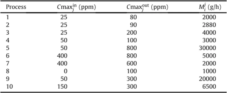
This example involving ten processes, one regeneration unit of type I (seeTable 1) and one contaminant, was already proposed by Bagajewicz and Savelski (2001), the corresponding limiting process data are shown inTable 2and the outlet regeneration concentra-tion is fixed at 5 ppm. The corresponding MILP involves 143 binary variables related to connections, 332 continuous variables and 351 constraints.
4.2. Theoretical results
The biobjective optimization was performed for different values of the connection number F3in the range [11, 120]. The constraint
(18) imposes to minimize the overall fresh water consumption. Hence, for several ranges of F2, the fresh water consumption is
minimized in order to have one optimal solution for each range of
F2and for a given value of F3. Starting from F3¼ 11, all the possible
values for F3were tested. When F3is greater or equal to 19, all the Table 1
Values ofaaccording to types of regeneration units.
Regeneration type Outlet concentration (ppm) avalue
I 50 0.375
II 20 1.75
fronts are superimposed on the same straight line. For example, the Pareto fronts corresponding to F3¼ 11, 12, 19 and 120 are reported
inFig. 2.Feng et al. (2007)show the linearity of the Pareto fronts for this particular problem. The values obtained for this example are identical with the ones reported in the literature (Bagajewicz and Savelski, 2001; Feng et al., 2008; Huang et al., 1999). Thus the network mathematical formulation and the optimization proce-dure are validated.
4.3. Choice of the best feasible network
The solutions displayed in Fig. 2are only theoretical results because in some cases, connections with quasi-null flow rates may exist. Obviously this type of solution cannot be considered in practice. Indeed, it is generally admitted (Bagajewicz and Savelski, 2001) that networks involving flows lower than 2 T h!1 cannot
be used in practice because they force the user using very small pipes (with a diameter of about 1 inch). These pipes are not economically profitable regarding their investment cost. From the theoretical study, “good” solutions on an industrial point of view, combining moderate GEC, few connections and non null flow rates
in the connections have to be defined. The minimum value of GEC was studied vs. the connection numbers, and the best solution (GEC ¼ 619 T h!1) is obtained with 17 connections and corresponds
to: F1¼ Fw¼ 10 T h!1and F2¼ 177 T h!1. The flowsheet of the
proposed solution is given inFig. 3(connections are numbered in brackets; connections going to the waster are not numbered). Other solutions with higher connection numbers can be also identified, but are topologically more complicated.
4.4. Discussion
From this example, the following conclusions can be empha-sized: (i) the solutions provided by the Pareto fronts are only theoretical results; ii) further investigations based on the global equivalent cost (GEC) and the connection number have to be per-formed for identifying the best practical solution; iii) since it does not requires any initialization phase and can tackle large scale problems, this MILP approach can be implemented to optimize EIPs, where the problems are larger in terms of numbers of vari-ables and constraints.
5. EIPs for managing industrial waters
5.1. Problem formulation
The DWN procedure is now extended to the design of EIPs and illustrated by the example proposed byOlesen and Polley (1996). The industrial pool involves three companies, each one including five processes; the data are displayed inTable 3.
The three companies decide to constitute an EIP for managing their used waters. Three scenarios are considered: EIP without regeneration unit, EIP where each company owns its regeneration unit and EIP where the three companies share regeneration unit(s). Three possible regeneration units (see Table 1) can be chosen under two kinds of constraints: limited or unlimited number of
Table 2
Process data for the water allocation problem. Process Cmaxin j (ppm) Cmaxoutj (ppm) M j i(g/h) 1 25 80 2000 2 25 90 2880 3 25 200 4000 4 50 100 3000 5 50 800 30000 6 400 800 5000 7 400 600 2000 8 0 100 1000 9 50 300 20000 10 150 300 6500
connections, same or different gains for each company. The objective is then to identify the best strategy for each company so as to minimize the global equivalent cost in fresh water and the number of connections in the network. Compared to some basic cases, a solution will be retained only if the gain in GEC for each
company is positive, and for two equivalent gains, the solution with a minimum ENC will be selected.Table 4explains the several cases which are explored all along the Section5. The results are displayed inTable 5, where only the cases giving a positive gain in GEC compared to the basic case for the three companies are re-ported. The rejected solutions are reported inTable 6and will not be discussed in the following sub-sections.
5.2. Basic case: companies without EIP and without regeneration unit (case 1)
This preliminary study (case 1) concerns the individual opti-mization of the water network for each company without consid-ering the EIP, according to objectives F1and F3(since there is no
regeneration unit, the objective F2is not taken into account). The
results of this monobjective optimization problem are displayed in Table 5, and for the sake of illustration, the network flowsheet for company A with six connections is displayed inFig. 4.
5.3. EIP without regeneration unit (cases 2e4)
The three companies which have no regeneration unit consti-tute an EIP without regeneration unit, but by allowing their used waters to be treated in the two other companies and receiving used
Fig. 3. Best solution for the water allocation problem (flows are in T/h).
Table 3
Process characteristics for the EIP. Process Company Contaminant
flow rate (Kg/h) Maximal inlet concentration (ppm) Maximal outlet concentration (ppm) 1 A 2 0 100 2 2 50 80 3 5 50 100 4 30 80 800 5 4 400 800 6 B 2 0 100 7 2 50 80 8 5 80 400 9 30 100 800 10 4 400 1000 11 C 2 0 100 12 2 25 50 13 5 25 125 14 30 50 800 15 15 100 150 Table 4
Characteristics of the cases treated.
Superstructure Cases Description of the configuration
Without EIP Case 1 Companies are considered individually and are not included in the EIP
Case 2 Connections are not included as an objective, F3is free
EIP without regeneration unit Case 3 Connections are restricted to 21, the minimum feasible
Case 4 Connections are restricted to 21 and each company needs to have the same gain Case 5 Companies are considered individually to choose their own regeneration unit EIP with individual regeneration units (direct integration scheme) Case 6 Connections are not included as an objective, F3is free
Case 7 Connections are restricted to 26, the minimum feasible
Case 8 Connections are restricted to 26 and each company needs to have the same gain Case 9 EIP with regeneration unit of type I
EIP with a shared regeneration unit (indirect integration scheme) Case 10 EIP with regeneration unit of type I and external connections are restricted to 2 Case 11 EIP with an interceptor containing regenerations of type I, II and III
Case 12 Case 11 with connections restricted to 26 and the same gain for each company Case 13 Case 11 with connections restricted to 31 and the same gain for each company Summarization of the several cases treated in Section6.
waters from the two other companies, as shown inFig. 5(do not take into account the dotted lines, nor italic parts). Three cases are considered: case 2 corresponds to an unlimited number of connections in the EIP; in case 3 the number of connections is assumed to be restricted to 21, which is the best solution found in case 1 (6 for company A, 8 for company B and 7 for company C, see Table 4); in case 4 the number of connections is also limited to 21 and the same relative gain is assumed for each company.
The results are displayed in Table 5, where the gains are computed by using case 1 as a basis. Only the case 4 (same relative
gain in GEC for each company, and also the same number of connections, 21), gives a positive gain (4.3%) for each company. The new flowsheet for company A in the case 4 is depicted inFig. 6, where external connections are numbered in brackets, italic.
5.4. EIP with one regeneration unit per company (direct integration, cases 5e8)
Each company is now equipped with its own regeneration unit chosen among the three types above mentioned. In the basic case 5, the DWN problem is solved for each company without considering the EIP in order to determine the best regeneration unit chosen among the three types listed inTable 1. From this multiobjective optimization study (objectives F1, F2and F3), the best solution is
obtained when companies A and B choose regeneration unit I, and company C, regeneration unit II. These solutions are given by the median points of the Pareto fronts (F1, F2) for the minimal values of
F3, and the results are displayed inTable 5.
Then the three companies constitute an EIP without common regeneration unit, but by allowing their polluted streams to be treated either in their own regeneration unit, or in the two other companies (seeFig. 5, do not take into account the dotted lines). Three new cases are considered: case 6 with no limitation on the number of connections, case 7 with the same number of connections less equal than the best solution of case 5 (26, i.e. 8 for
Table 5
Results for the EIP (only cases with positive gains are reported).
Case F1T/h FwT/h F2T/h GEC T/h Gain %
Case 1 Gain % Case 5 Int. + Ext. conn A case 1 98.3 98.3 xxx 651 xxx xxx 6 A case 4 102.8 92.6 xxx 623 4.3 Xxx 6 A case 5 20 20 166 195 70.0 xxx 8 A case 8 20 15.2 166.6 168 74.2 13.8 7 A case 13 20 19 166 188 71.1 3.6 9 B case 1 54.6 54.6 xxx 362 xxx xxx 8 B case 4 45 53.6 xxx 346 4.3 xxx 6 B case 5 20 20 66.7 157 56.6 xxx 8 B case 8 20 12 128 135 62.4 13.8 9 B case 13 20 19 67 151 76.8 3.6 12 C case 1 190 190 xxx 1259 Xxx xxx 7 C case 4 180 182 xxx 1204 4.3 xxx 9 C case 5 20 20 192 469 62.7 xxx 10 C case 8 20 32.7 114 404 67.9 13.8 10 C case 13 20 22 213 452 30.6 3.6 10 Total case 1 343 343 xxx 2272 xxx xxx 21 Total case 4 328 328 xxx 2173 4.3 xxx 21 Total case 5 60 60 426 821 63.9 xxx 26 Total case 8 60 60 409 708 68.8 13.8 26 Total case 13 60 60 446 791 65.2 3.6 31 Table 6 Rejected solutions.
Rejected solution Gain % vs. Case 1 Gain % vs. Case 5
C case 2 !8.2 xxx B case 3 !10.5 xxx C case 3 !2.6 xxx A case 6 xxx !10.2 B case 6 xxx !61.8 A case 7 xxx !74.9 A case 9 xxx !144.6 B case 10 xxx !233.1 B case 11 xxx !138.2 A case 12 xxx !7.7 B case 12 xxx !7.7 C case 12 xxx !7.7
companies A and B and 10 for company C, seeTable 5), case 8 with the same relative gain in GEC (compared with case 5) for each company, and also the number of connections less equal to 26.
The results are displayed inTable 5, where the gains in GEC are computed by using case 1, then case 5 as a basis. Case 5 being the basis of comparison, only case 8 provides positive a positive gain for each company (same gain of 13.8%, number of connections equal to 26); it is the best solution for the EIP. The new flowsheet for company A in this solution is depicted inFig. 7. Compared with case 1, regeneration units (cases 5 and 8) provide very interesting gains (63.9 and 68.8%). The economic interest of regeneration units is evident. It may be interpreted thatTable 5exhibits inconsistent results between waste and regenerated flows for cases B8, (increase (decrease) in waste and increase (decrease) in regeneration). This is yet not the case since included into an EIP a company may reject or regenerate waters coming from other companies.
5.5. EIP with a common regeneration unit (indirect integration, cases 9e13)
The three companies have now an interceptor containing shared regeneration unit(s) and connections between them (seeFig. 5, do not take into account the italic parts). Five cases are evaluated. Case 9 corresponds to an unlimited number of connections and a shared
Fig. 5. Representation of an EIP for the three companies (fromChew et al., 2008) (straight lines: direct integration, dash lines: indirect integration).
Fig. 6. Network for company A (case 4) (flows are in T/h, numbers of pipes are in brackets, external connections are in italic).
regeneration unit of type I. In case 10, the number of external connections between companies is limited at two pipes and a shared regeneration unit of type I is used. Case 11 concerns an EIP involving an interceptor containing the three types of regeneration units, each company can choose two units among the three possible ones, and unlimited number of connections. Case 12 is deduced from case 11 by restricting the total number of connections to 26 (as in cases 7 and 8) and assuming the same gain for each company (compared with case 5), and finally in case 13, the same gain for each company is also imposed but the total number of connections is arbitrarily increased to 31.
Compared with case 5, only case 13 gives a positive gain for each company (3.6%), but compared with the best solution, case 8, found in the previous example the gain for each company is negative (!11.7%). In conclusion, the EIP involving an interceptor is not economically profitable.
5.6. Discussion
This study shows first that regeneration units yield very significant gains, and second that these gains can be increased again by a direct integration into an EIP. Finally the a priori most attractive EIP with an indirect integration (interceptor sharing regeneration units) does not succeed in improving the previous solution. The best EIP (case 8) is shown inFig. 8(the connections to the waste are not reported), and the flowsheet of company A in this EIP is depicted inFig. 7.
6. Computational aspects
For all the cases, the problem dimensions are displayed in Table 7. When passing from a DWN problem (case 1) to EIP prob-lems, the dimensions strongly increase. However due to the linear formulation this increase has not much influence either on the problem resolution, or on the CPU time (the computations were carried on an Intel Duo Core 2.53 GHz, RAM 3.45 Go). The MILP problem is solved with the solver CPLEX 11.2.1 of the GAMS package.
7. Conclusions
In the first part of the paper, a methodology taking into account only the single contaminant case is implemented. A MILP formu-lation is used to solve the problem. Biobjective optimization of the fresh water flow rate at the network entrance and the water flow rate at regeneration unit inlets, parameterized by the number of connections in the network, is carried out. A strategy based on the global equivalent cost (GEC) and equivalent number of connections (ENC) allows identifying the best practical solution combining moderate GEC, few connections and non null flow rates in the connections, among the theoretical ones displayed on Pareto fronts. This MILP approach is then implemented to optimize an EIP involving three companies. From several analyzed scenarios, it can be deduced that the best solution is an EIP with direct integration: each company owns its regeneration unit, same gain for each company and restricted number of connections. Compared with the case of companies without EIP and without regeneration unit, the gain in GEC is 68.8%, and compared with the case of companies without EIP, but with their own regeneration unit, the supple-mentary gain in GEC for each company is 13.8%. This study shows first that regeneration units yield very significant gains, and second that these gains can be increased again by a direct integration into an EIP. Finally, the a priori most attractive EIP with an indirect integration (interceptor sharing regeneration units) does not succeed in improving the previous solution. Using different criteria (GEC, connections number, non null flow rates in the connections), a best practical solution is defined for each case. Moreover, after optimisation, the gain for each case is calculated and each company in the EIP can decide to connect to the EIP or not. Of course, the
Fig. 8. EIP solution (case 8, flows are in T/h).
Table 7
Problem dimensions and CPU times. Problem Continuous variables Integer variables Constraints CPU time (s) Case 1 173 47 214 0.063 Case 2e4 836 255 900 0.109 Case 5e8 1164 357 1312 0.140 Case 9e13 1164 357 1319 0.250
calculated gain is different in each case, so it is easier to choose the type of connections. Due to the MILP problem, it is possible to add some technical constraints without any size limitations.
Few studies were realized on the technical constitution of an EIP, and even less in the framework of multiobjective optimization, while the problem is by nature a multiobjective one, combining economical and ecological objectives. Furthermore, in a recent studySakr et al. (2011)identify seven success and limiting factor for EIPs development. The present study comes within the second one “Added economic value”, and fills partially the existing gap in the literature.
References
Alexander, B., Barton, G., Petrie, J., Romagnoli, J., 2000. Process synthesis and optimisation tools for environmental design: methodology and structure. Comp. Chem. Eng. 24, 1195e1200.
Allenby, B., 2006. The ontologies on industrial ecology. Prog. Ind. Ecol. Int. J. 3 (1e2), 28e40.
Aviso, K.B., Tan, R.R., Culaba, A.B., 2010a. Designing eco-industrial water exchange networks using fuzzy mathematical programming. Clean Technol. Environ. Policy 12, 353e363.
Aviso, K.B., Tan, R.R., Culaba, A.B., Cruz Jr., J.B., 2010b. Bi-level fuzzy optimization approach for water exchange in eco-industrial parks. Process Saf. Environ. Prot. 88, 31e40.
Baas, L., 2006. Cleaner production systems in the context of needed partners and policies at the micro, meso and macro level. UNIDO Cleaner Production Expert Group Meeting, Baden, Austria, pp. 29e31 October 2006.
Baas, L., Boons, F., 2004. An industrial ecology project in practice: exploring the boundaries of decision-making levels in regional industrial systems. J. Clean Prod. 12, 1073e1085.
Bagajewicz, M., Faria, D.C., 2009. On the appropriate architecture of the water/ wastewater allocation problem in process plants. Comput. Aided Chem. Eng. 26, 1e20.
Bagajewicz, M., Savelski, M., 2001. On the use of linear models for the design of water utilization systems in process plants with a single contaminant. Chem. Eng. Res. Des. 79, 600e610.
Boix, M., Montastruc, L., Pibouleau, L., Azzaro-Pantel, C., Domenech, S., 2010. Mul-tiobjective optimization of industrial water networks with contaminants. Comput. Aided Chem. Eng. 28, 859e864.
Boix, M., Montastruc, L., Pibouleau, L., Azzaro-Pantel, C., Domenech, S., 2011. A multiobjective optimization framework for multicontaminant industrial water network design. J. Environ. Manage. 92, 1802e1808.
Côté, R., Cohen-Rosenthal, E., 1998. Designing eco-industrial parks: a synthesis of some experiences. J. Clean Prod. 6, 181e188.
Chertow, M.R., 2000. Industrial symbiosis: literature and taxonomy. Annu. Rev. Energy Env. 25, 313e337.
Chertow, M.R., 2007. Uncovering" industrial symbiosis. J. Ind. Ecol. 11, 11e30. Chew, I.M.L., Tan, R.R., Ng, D.K.S., Foo, D.C.Y., Majozi, T., Gouws, J., 2008. Synthesis of
direct and indirect interplant water network. Ind. Eng. Chem. Res. 47, 9485e9496.
Chew, I.M.L., Tan, R.R., Foo, D.C.Y., Chiu, A.S.F., 2009. Game theory approach to the analysis of interplant water integration in an eco-industrial park. J. Clean Prod. 17, 1611e1619.
Chew, I.M.L., Foo, D.C.Y., Ng, D.K.S., Tan, R.R., 2010a. Flowrate targeting algorithm for interplant resource conservation network. Part 1: unassisted integration scheme. Ind. Eng. Chem. Res. 49, 6439e6455.
Chew, I.M.L., Foo, D.C.Y., Tan, R.R., 2010b. Flowrate targeting algorithm for interplant resource conservation network. Part 2: assisted integration scheme. Ind. Eng. Chem. Res. 49, 6456e6468.
Chew, I.M.L., Thillaivarrna, S.L., Tan, R.R., Foo, D.C.Y., 2010c. Analysis of inter-plant water integration with indirect integration schemes through game theory approach: pareto optimal solution with interventions. Clean Technol. Environ. Policy 13, 49e62.
Conover, W.R., 1918. Salvaging and utilizing wastes and scrap in industry. Ind. M. 55.6, 449e451.
de Faria, D.C., de Souza, A.A.U., Guelli Ulson de Souza, S.M.A., 2009. Optimization of water networks in industrial processes. J. Clean Prod. 17, 857e862.
Dunn, R.F., Wenzel, H., 2001. Process integration design methods for water conser-vation and wastewater reduction in industry. Clean. Prod. Processes 3, 307e318. El-Halwagi, M.M., 1997. Pollution Prevention through Process
Integra-tiondSystematic Design Tools. Academic Press, CA, USA.
El-Halwagi, M.M., Gabriel, F., Harell, D., 2004. Rigorous graphical targeting for resource conservation via material recycle/reuse networks. Ind. Eng. Chem. Res. 42, 4319e4328.
Erol, P., Thöming, J., 2005. ECO-design of reuse and recycling networks by multi-objective optimization. J. Clean Prod. 13, 1492e1503.
Feng, X., Bai, J., Zheng, X.S., 2007. On the use of graphical method to determine the targets of single contaminant regeneration recycling water systems. Chem. Eng. Sci. 62, 2127e2138.
Feng, X., Bai, J., Wang, H.M., Zheng, X.S., 2008. Grass-roots design of regeneration recycling water networks. Comp. Chem. Eng. 32, 1892e1907.
Frosh, R.A., Gallopoulos, N.E., 1989. Strategies for manufacturing. Sci. Am. 261, 144e152.
Galan, B., Grossmann, I.E., 1998. Optimal design of distributed wastewater treat-ment networks. Ind. Eng. Chem. Res. 37, 4036e4048.
Geng, Y., Hengxin, Z., 2009. Industrial park management in the Chinese environ-ment. J. Clean Prod. 17, 1289e1294.
Gibbs, D., Deutz, P., 2005. Implementing industrial ecology? Planning for eco-industrial parks in the USA. Geoforum 36, 452e464.
Gibbs, D., Deutz, P., 2007. Reflections on implementing industrial ecology through eco-industrial park development. J. Clean Prod. 15, 1683e1695.
Giurco, D., Bossilkov, A., Patterson, J., Kazaglis, A., 2010. Developing industrial water reuse synergies in Port Melbourne: cost effectiveness, barriers and opportuni-ties. J. Clean Prod. 19, 867e876.
Gomes, F.S., Queiroz, E.M., Pessoa, F.L.P., 2007. Design procedure for water/waste-water minimization: single contaminant. J. Clean Prod. 15, 474e485. Gussow, D., Meyers, J., 1970. Industrial Ecology, vol. 1.
Hallale, N., Fraser, D.M., 2000. Super-targeting for mass exchange networks. Part I: targeting and design techniques. Trans. Inst. Chem. Eng. 78, 202e216. Heeres, R.R., Vermeulen, W.J.V., de Walle, F.B., 2004. Eco-industrial parks
initiatives in the USA and the Netherlands: first lessons. J. Clean Prod. 12, 985e995.
Hoffman, C., 1971. The Industrial Ecology of Small and Intermediate-sized Technical Companies: Implications for Regional Economic Development. Report Prepared for the Economic Development Administration COM-74-10680. Texas Univer-sity, USA.
Huang, C.H., Chang, C.T., Ling, H.C., Chang, C.C., 1999. A mathematical programming model for water usage and treatment network design. Ind. Eng. Chem. Res. 38, 2666e2679.
Jacob, J., Viviant, C., Houle, H.F., Paris, J., 2002. Analysis and optimization of water networks in pulp and paper manufacturing: pinch technology. Pulp Pap. Can. 103, 24e27. In French.
Karuppiah, R., Grossmann, I.E., 2008. Global optimization of multiscenario mixed integer nonlinear programming models arising in the synthesis of integrated water networks under uncertainty. Comp. Chem. Eng. 32, 145e160.
Kim, S.H., Yoon, S.-G., Chae, S.H., Park, S., 2010. Economic and environmental optimization of a multi-site utility network for an industrial complex. J. Environ. Manage. 91, 690e705.
Klemes, J., Friedler, F., Bulatov, I., Varbanov, P., 2010. Sustainability in the Process Industry e Integration and Optimization. McGraw-Hill, New York, USA. Kumaraprasad, G., Muthukumar, K., 2009. Design of mass exchange network and
effluent distribution system for effective water management. J. Clean Prod. 17, 1580e1593.
Lavric, V., Iancu, P., Plesu, V., 2005. Genetic algorithm optimisation of water consumption and wastewater network topology. J. Clean Prod. 13, 1405e1415. Lim, S.R., Park, J.M., 2008. Cooperative water network system to reduce carbon
footprint. Environ. Sci. Technol. 42, 6230e6236.
Linnhoff, B., Vredeveld, R., 1984. Pinch technology has come of age. Chem. Eng. Prog., 33e40.
Liu, C., Zhang, K., Zhang, J., 2010. Sustainable utilization of regional water resources: experiences from the Hai Hua ecological industry pilot zone (HHEIPZ) project in China. J. Clean Prod. 18, 447e453.
Liwarska-Bizukojc, E., Bizukojc, M., Marcinkowski, A., Doniec, A., 2009. The conceptual model of an eco-industrial park based upon ecological relationships. J. Clean Prod. 17, 732e741.
Lovelady, E.M., El-Halwagi, M.M., 2009. Design and integration of eco-industrial parks for managing water resources. Environ. Prog. Sustain. Energy 28, 265e272.
Manan, Z.A., Wan Alwi, S.R., Ujang, Z., 2006. Water pinch analysis for an urban system: a case study on the Sultan Ismail Mosque at the Universiti Teknologi Malaysia (UTM). Desalination 194, 52e68.
Mavrotas, G., 2009. Effective implementation of the ε-constraint method in multi-objective mathematical programming problems. Appl. Math. Comput. 213, 455e465.
Mirata, M., 2004. Experiences from early stages of a national industrial symbiosis programme in the UK: determinants and coordination challenges. J. Clean Prod. 12, 967e983.
Oecd, 2008. Organisation for Economic Co-Operation and Development. OECD Environmental Outlook to 2030, Paris, France.
Oh, D.S., Kim, K.B., Jeong, S.Y., 2005. Eco-industrial park design: a Daedeok Tech-novalley case study. Habitat Int. 29, 269e284.
Olesen, S.G., Polley, G.T., 1996. Dealing with plant geography and piping constraints in water network design. Process Saf. Environ. Prot. 74, 273e276.
PCSD (President’s Council on Sustainable Development), 1996. Eco-Efficiency Task Force Report Washington, D.C, USA.
Park, H.S., Rene, E.R., Choi, S.M., Chiu, A.S.F., 2008. Strategies for sustainable development of industrial park in Ulsan, South Korea - from spontaneous evolution to systematic expansion of industrial symbiosis. J. Environ. Manage. 87, 1e13.
Poplewski, G., Walczyk, K., Jezowski, J., 2010. Optimization-based method for calculating water networks with user specified characteristics. Chem. Eng. Res. Des. 88, 109e120.
Quesada, I., Grossmann, I.E., 1995. Global optimization of bilinear process networks with multicomponent flows. Comp. Chem. Eng. 19, 1219e1242.
Roberts, B.H., 2004. The application of industrial ecology principles and planning guidelines for the development of eco-industrial parks: an Australian case study. J. Clean Prod. 12, 997e1010.
Sahinidis, N.V., 2004. Optimization under uncertainty: state-of-the-art and oppor-tunities. Comp. Chem. Eng. 28, 971e983.
Sakr, D., Bass, L., El-Haggar, S., Huisingh, R., 2011. Critical success and limiting factors for eco-industrial parks: global trends and Egyptian context. J. Clean Prod. 19, 1158e1165.
Savelski, M., Bagajewicz, M., 2000. On the necessary conditions of water utilization systems in process plants with single contaminants. Chem. Eng. Sci. 55, 5035e5048. Shafiei, S., Domenech, S., Koteles, R., Paris, J., 2004. System closure in pulp and paper
mills: network analysis by genetic algorithm. J. Clean Prod. 12, 131e135. Shi, H., Chertow, M., Song, Y., 2010. Developing country experience with
eco-industrial parks: a case study of the Tianjin Economical-Technological Devel-opment Area in China. J. Clean Prod. 18, 191e199.
Sienutycz, S., Jezowski, J., 2009. Energy Optimization in Process Systems e Chapter 20: Approaches to Water Network Design. Elsevier, Oxford, UK, ISBN 0-08-045141-1. 613e657.
Simmonds, P.L., 1862. Waste Products and Undeveloped Substances. Hardwicke, London.
Tibbs, H.B.C., 1993. Industrial Ecology. An Environmental Agenda for Industry. Global Business Network, Emeryville, CA.
Tiejun, D., 2010. Two quantitative indices for the planning and evaluation of eco-industrial parks. Res. Conserv. Recycle 54, 442e448.
Tudor, T., Adam, E., Bates, M., 2007. Drivers and limitations for the successful development and functioning of EIPs (eco-industrial parks): a literature review. Ecol. Econ. 61, 199e207.
UNESCO, Paris and Earthscan, London, 2009. World Water Assessment Programme. The United Nations World Water Development Report 3: Water in a Changing World.
Van Beers, D., Corder, G., Bossilkov, A., Van Berkel, R., 2007. Industrial symbiosis in the Australian minerals industry: the cases of Kwinana and Gladstone. J. Ind. Ecol. 11, 55e72.
Van Berkel, R., 2007. Cleaner production and eco-efficiency initiatives in Western Australia 1996e2004. J. Clean Prod. 15, 741e755.
Van Leeuwen, M.G., Vermeulen, W.J.V., Glasbergen, P., 2003. Planning eco-industrial parks: an analysis of Dutch planning methods. Bus. Strat. Environ. 12, 147e162. Veiga, E., Bechara, L., Magrini, A., 2009. Eco-industrial park development in Rio de Janeiro, Brazil: a tool for sustainable development. J. Clean Prod. 17, 653e661. Wang, Y.P., Smith, R., 1994. Wastewater minimization. Chem. Eng. Sci. 49,
981e1006.
Wan Alwi, S.R., Manan, Z.A., Samingin, M.H., Misran,., N., 2008. A holistic framework for design of cost-effective minimum water utilization network. J. Environ. Manage. 88, 219e252.
Watanabe, C., 1972. Industrial-Ecology: Introduction of Ecology into Industrial Policy. Ministry of International Trade and Industry (MITI), Tokyo.
Zhu, L., Zhou, J., Cui, Z., Liu, L., 2010. A method for controlling enterprises access to an eco-industrial park. Sci. Total Environ. 408, 4817e4825.