HAL Id: hal-02051580
https://hal.archives-ouvertes.fr/hal-02051580v2
Preprint submitted on 27 May 2019 (v2), last revised 20 Nov 2019 (v3)
HAL is a multi-disciplinary open access
archive for the deposit and dissemination of
sci-entific research documents, whether they are
pub-lished or not. The documents may come from
teaching and research institutions in France or
abroad, or from public or private research centers.
L’archive ouverte pluridisciplinaire HAL, est
destinée au dépôt et à la diffusion de documents
scientifiques de niveau recherche, publiés ou non,
émanant des établissements d’enseignement et de
recherche français ou étrangers, des laboratoires
publics ou privés.
Attention Based Pruning for Shift Networks
Ghouthi Boukli Hacene, Carlos Lassance, Vincent Gripon, Matthieu
Courbariaux, Yoshua Bengio
To cite this version:
Ghouthi Boukli Hacene, Carlos Lassance, Vincent Gripon, Matthieu Courbariaux, Yoshua Bengio.
Attention Based Pruning for Shift Networks. 2019. �hal-02051580v2�
Attention Based Pruning for Shift Networks
Ghouthi Boukli Hacene1,2, Carlos Lassance1,2, Vincent Gripon1,2
Matthieu Courbariaux1and Yoshua Bengio1 1Université de Montréal, MILA,2IMT Atlantique, Lab-STICC
Abstract
In many application domains such as computer vision, Convolutional Layers (CLs) are key to the accuracy of deep learning methods. However, it is often required to assemble a large number of CLs, each containing thousands of parameters, in order to reach state-of-the-art accuracy, thus resulting in complex and demanding systems that are poorly fitted to resource-limited devices. Recently, methods have been proposed to replace the generic convolution operator by the combination of a shift operation and a simpler 1x1 convolution. The resulting block, called Shift Layer (SL), is an efficient alternative to CLs in the sense it allows to reach similar accuracies on various tasks with faster computations and fewer parameters. In this contribution, we introduce Shift Attention Layers (SALs), which extend SLs by using an attention mechanism that learns which shifts are the best at the same time the network function is trained. We demonstrate SALs are able to outperform vanilla SLs (and CLs) on various object recognition benchmarks while significantly reducing the number of float operations and parameters for the inference.
1
Introduction
Convolutional Neural Networks (CNNs) are the state-of-the-art in many computer vision tasks, such as image classification, object detection and face recognition Szegedy et al. [2016]. To achieve top-rank accuracy, CNNs rely on the use of a large number of trainable parameters, and considerable computational complexity. This is why there has been a lot of interest in the past few years towards the compression of CNNs, so that they can be deployed onto embedded systems. The purpose of compressing DNNs is to reduce memory footprint and/or computational complexity while mitigating losses in accuracy.
Prominent works to compress neural networks include binarizing (or quantifying) weights and activa-tions Courbariaux et al. [2015], Soulié et al. [2016], Rastegari et al. [2016], Lin et al. [2015], Li et al. [2016a], Zhou et al. [2016], Han et al. [2015a], Wu et al. [2018], pruning network connections during or before training Han et al. [2015a,b], Li et al. [2016b], Ardakani et al. [2016], using grouped convolu-tions Chollet [2017], Howard et al. [2017], Sandler et al. [2018], introducing new components Zhang et al. [2018], Juefei-Xu et al. [2017], using convolutional decomposition Szegedy et al. [2015], Simonyan and Zisserman [2014], or searching for a lightweight neural network architecture Iandola et al. [2016].
Recently, the authors of Wu et al. [2017] have proposed to replace the generic convolution operator with the combination of shifts and simpler 1x1 convolutions. In their work, the shifts are hand-crafted and all the parameters to be trained are in the 1x1 convolutions. These operations are particularly well suited to embedded devices Hacene et al. [2018], Yang et al. [2018].
In this paper, we introduce the Shift Attention Layer (SAL), which can be seen as a selective shift layer. Indeed, the proposed layer starts with a vanilla convolution and learns to transform it into a shift layer throughout the training of the network function. It uses an attention mechanism Vaswani et al. [2017] that selects the best shift for each feature map of the architecture, what can be seen as
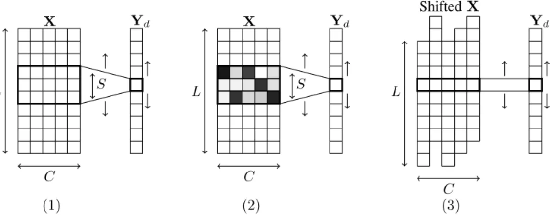
L C (1) S X Yd L C (2) S X Yd L Shifted X Yd C (3)
Figure 1: Overview of the proposed method: we depict here the computation for a single output feature map d, considering a 1d convolution and its associated shift version. Panel (1) represents a standard convolutional operation: the weight filter Wd,·,·containing SC weights is moved along the
spatial dimension (L) of the input to produce each output in Yd. In panel (2), we depict the attention
tensor A on top of the weight filter: the darker the cell, the most important the corresponding weight has been identified to be. At the end of the training process, A should contain only binary values with a single 1 per slice Ad,c,·. In panel (3), we depict the corresponding obtained shift layer: for
each slice along the input feature maps (C), the cell with the highest attention is kept and the others are disregarded. As a consequence, the initial convolution with a kernel size S has been replaced by a convolution with a kernel size 1 on a shifted version of the input X. As such, the resulting operation in panel (3) is exactly the same as the shift layer introduced in Wu et al. [2017], but here the shifts have been trained instead of being arbitrarily predetermined.
a pruning technique. We demonstrate it is able to significantly outperform original shift layers Wu et al. [2017] and other pruning techniques at the cost of requiring more parameters during training, but ends up with less parameters for inference. It is thus of particular interest for implementing the inference process on resource-limited systems.
The outline of the paper is as follows. In Section 2 we explain the proposed method. In Section 3 we present related work. In Section 4 we present experiments on challenging computer vision datasets. Finally, In Section 5 we discuss future work and conclude. All the code used to run the experiments in this paper is available online: https://hiddenduringreviewing.
2
Methodology
In this section, we first review the classical spatial convolution operation and see how it can be related to the shift operation defined in Wu et al. [2017]. We then introduce our proposed method.
2.1 Convolution/Shift operation
Let us consider the 1d case (other cases can be easily derived). Let us denote by X ∈ RC×Lan input tensor of a convolutional layer, where C is the number of channels and L is the dimension of each feature map (a.k.a. spatial dimension). We denote W ∈ RD×C×Sthe corresponding weight tensor,
where D is the number of output channels, S the kernel size, and Y ∈ RD×Lthe output tensor. Disregarding padding (i.e. border effects), the convolution operation is defined through Equation (1) and depicted in Figure 1, panel (1).
yd,`= C X c=1 S X `0=1 xc,`+`0−dS/2ewd,c,`0, ∀d, ` . (1)
A shift layer is obtained when connections in W are pruned so that exactly one connection remains for each slice Wd,c,·, ∀d, c. We denote `d,cthe index such that wd,c,`d,cis not pruned. Then the shift
yd,` = C X c=1 xc,`+`d,c−dS/2ewd,c,`d,c (2) = C X c=1 ˜ xc,`w˜d,c, (3)
where ˜xc,`= xc,`+`d,c−dS/2eand ˜wd,c= wd,c,`d,c. We observe that the shift operation boils down to
shifting the input tensor X then convoluting with a kernel of size 1 (in the equation, the kernel ˜W is indexed only by the input and output feature maps). In the original work Wu et al. [2017], the authors proposed to arbitrarily predetermine which shifts are used before training the architecture. To the contrary, in this work, we propose a method that learns which shifts to perform during the training process.
2.2 Shift Attention Layer (SAL)
The idea we propose is to enrich a classical convolution layer with a selective tensor A which aims at identifying which connections should be kept in each slice of the weight tensor. As such, we introduce A ∈ RD×C×La tensor containing as many elements as weights in the weight tensor. Each value of A is normalized between 0 and 1 and represents how important the corresponding weight in W is (c.f. Figure 1: panel (2)) with respect to the task to be solved. At the end of the training process, A becomes binary, with only one nonzero element per slice Ad,c,·, corresponding to the weights in
W that should be kept.
More precisely, each slice Ad,c,·is normalized using a softmax function with temperature T . The
temperature is decreased smoothly along the training process. Note that in order to force the mask A to be selective, we first normalize each slice Ad,c,·so that it has 1 standard deviation (sd). Algorithm 1
summarizes the training process of one layer. At the end of training, the selected weight in each slice Wd,c,·corresponds to the maximum value in Ad,c,·.
Algorithm 1 SAL algorithm of one layer Inputs: Input tensor X,
Initial softmax temperature T , Constant α < 1. for each training iteration do
T ← αT for d := 1 to D do for c := 1 to C do Ad,c,·← Ad,c,· sd(Ad,c,·) Ad,c,·← Sof tmax(T Ad,c,·) end for end for
WA← W · A (· is the pointwise multiplication)
Compute standard convolution as described in Equation 1 using input tensor X and weight tensor WAinstead of W .
Update W and A via back-propagation. end for
Note that contrary to the vanilla shift layers where the same number of shifts is performed in every direction, at the end of the training process the resulting shift layer can have an uneven distribution of shifts (c.f. Section 4). This comes with a price, which corresponds to the memory needed to retain which shift is performed for each input feature map. In order to be fair, we thus reduce the number of feature maps in the networks we use in the experiments so that the total memory is comparable. In the next section we present related works, thus our proposed method can easily be compared to previously introduced methods.
3
Related Work
Let us introduce related works aiming at reducing complexity and memory footprints of CNNs. In a first line of works, authors have proposed to binarize weights and activations Courbariaux et al. [2015, 2016], Rastegari et al. [2016], and then replace all multiplications by low cost multiplexers. Other works have proposed to use K-means to quantize weights Han et al. [2015b], Ullrich et al. [2017], Wu et al. [2018] and thus reduce the model size of CNNs.
Another line of work relies on network pruning Han et al. [2015a]. For example Li et al Li et al. [2016b] use the sum of absolute weights of each channel to select and prune redundant ones. In the same vein, He et al He et al. [2018] proposed a novel Soft Filter Pruning (SFP) approach to prune dynamically filters in a soft manner. Using the reconstruction error of the last layer before classification, Yu et al Yu et al. [2018] introduce the Neuron Importance Score Propagation (NISP) method. The main idea is to estimate the importance of each neuron in each layer in the backward propagation of the scores obtained from the reconstructed error. Huang et al Huang et al. [2018] propose a reinforcement learning based method, in which an agent is trained to maximize a reward function in order to improve the accuracy when pruning selected channels. Yamamoto et al Yamamoto and Maeno [2018] use a channel-pruning technique based on attention statistics by adding attention blocks to each layer and updating them during the training process to evaluate the importance of each channel. Compared to these works, the method we propose can be seen as a structured pruning technique in which most of the weights of a convolution are pruned but one per slice.
For mobile applications with limited resources, specific neural network architectures have been introduced. Iandola et al Iandola et al. [2016] propose a fire module to define SqueezeNet, a very small neural network with an acceptable accuracy. In Howard et al. [2017], Sandler et al. [2018], the authors use depthwise separable convolutions to define MobileNet and build lightweight CNNs. Other approaches focus on a decomposition of the convolution. Simonyan et al Simonyan and Zisserman [2014] reduce the number of parameters of VGG by replacing a 5 × 5 convolutions by two 3 × 3 convolutions each. In Szegedy et al. [2016], the authors decompose 7 × 7 convolutions into 1 × 7 and 7 × 1 convolutions. Our proposed work builds upon Wu et al Wu et al. [2017], where the authors introduce a shift operation, that we call shift layers throughout this article, as an alternative to spatial convolutions. The authors deconstruct 3 × 3 spatial convolutions into the concatenation of a shift transform on the input and 1 × 1 convolutions. As such, they are able to considerably reduce the complexity and memory usage of CNNs. In Hacene et al. [2018], the authors show it is possible to exploit this procedure for specific hardware targets. In Jeon and Kim [2018], the authors propose an active shift layer (ASL) that improves the accuracy of the shift operation method, and replaces the fixed handcrafted integer parameters of the shift layers by learned floating point parameters. Consequently, the result architecture requires to perform interpolations and does not fall into the original shift layer formulation.
In this contribution, we introduce Shift Attention Layers (SALs), a novel pruning-shift operation method that ends up replacing convolutions with shift layers by the end of training. Contrary to Jeon and Kim [2018], the proposed methodology result in a network that is exactly as described in Wu et al. [2017], with the main difference that shifts are learned instead of being predetermined. We demonstrate in this paper that it results in better accuracy for the exact same complexity and number of parameters.
4
Experiments
In this section we present the benchmark protocol used to evaluate the proposed method, and then compare the obtained performance with a CNN baseline, pruning methods and vanilla shift layers. 4.1 Benchmark Protocol
We evaluate using three object recognition datasets: CIFAR10, CIFAR100 and ImageNet ILSVRC 2012. To be comparable with the relevant literature, we use the same architectures from previous papers Yamamoto and Maeno [2018], Wu et al. [2017], Jeon and Kim [2018], that is Resnet-20/56 on CIFAR10 and Resnet-20/50 on CIFAR100 using the following parameters: the training process
Table 1: Comparison of accuracy and number of parameters between the baseline architecture (ResNet20), ShiftNet, ASNet, and SANet (the proposed method) on CIFAR10 and CIFAR100.
CIFAR10 CIFAR100
Accuracy Params (M) Accuracy Params (M)
CLs Baseline 94.66% 1.22 73.7% 1.24
SLs ShiftNet Wu et al. [2017] 93.17% 1.2 72.56% 1.23 SANet (ours) 95.52% 0.98 77.39% 1.01 Interpolate ASNet Jeon and Kim [2018] 94.53% 0.99 76.73% 1.02
Table 2: Comparison of accuracy, number of parameters and number of floating point operations (FLOPs) between baseline architecture (Resnet-56), SANet (the proposed method) , and some other pruning methods on CIFAR10. Note that the number between () refers to the result obtained by the baseline used for each method.
CIFAR10
Accuracy Params (M) FLOPs (M) Pruned-B Li et al. [2016b] 93.06%(93.04) 0.73(0.85) 91(126) Pruning NISP Yu et al. [2018] 93.01%(93.04) 0.49(0.85) 71(126) PCAS Yamamoto and Maeno [2018] 93.58%(93.04) 0.39(0.85) 56(126) SANet (ours) 94%(93.04) 0.36(0.85) 42(126)
consists of 300 epochs for Resnet-20 and 400 epochs for Resnet-50/56, the learning rate starts at 0.1 and is divided by 10 after each 100 epochs.
For the evaluations using CIFAR10 or CIFAR100 He et al. [2016], the training batch size is 128, the initial/final softmax temperatures are 6.7/0.02, and the temperature is multiplied at each step by α = 0.99994, 0.99996 when using 300, 400 epochs respectively. For ImageNet ILSVRC 2012, we used Resnet-w32 and Resnet-w64 defined in Jeon and Kim [2018] using the following parameters: the total number of epochs is 90, the training batch size is 1024, the learning rate starts at 0.1 and is divided by 10 after each 30 epochs, initial/final softmax temperatures are 6.7/0.016 so that the temperature update at each step is α = 0.99995. We also used standard data augmentation defined in Krizhevsky et al. [2012].
Let us point out that the values of temperatures were obtained by using a grid search. The fact the final temperature is not zero means that the tensors A may contain nonbinary values. This is why we binarize A using a hard max to obtain the corresponding shift layers before evaluating on the test set.
4.2 Results
The first experiment consists in comparing the accuracy, memory and number of operations of the proposed method compared to other shift layer based methods and pruning methods. We run tests using CIFAR10 and CIFAR100. Table 1 shows that our method achieves a better accuracy with fewer parameters than the baseline and other shift-module based methods. Tables 2 and 3 show that the proposed method is comparable or better in term of accuracy and number of parameters/floating point operations (FLOPs) with other pruning methods.
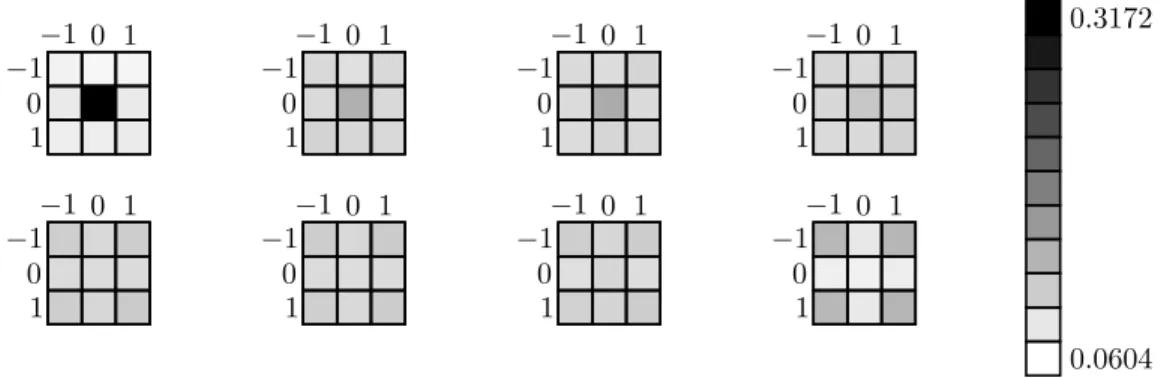
As mentioned in Section 2, the number of shifts in each direction can be uneven at the end of the training procedure. As such, in a second run of experiments, we look at the proportions of each shifts (relative position in kernel) depending on the layer depth in the architecture. In Figure 2, a heat-map represents the distribution of kept weights at different relative positions through Wd,c,·,·, ∀d, c slices,
for the 4 first layers (first row), and the 4 last layers (second row), of Resnet-20 trained on CIFAR10, where attention tensors A values are initially drawn uniformly at random. We observe that at the end of the training process, first layers seem to yield a uniform distribution of kept weights. To the contrary, for the last layers, there is a clear asymmetry that favours corners. This interestingly suggests that shift-layers would benefit from a non regular number of shifts in each direction.
Table 3: Comparison of accuracy, number of parameters and number of floating point operations (FLOPs) between baseline architecture (Resnet-50), SANet (the proposed method) , and some other pruning methods on CIFAR100. Note that the number between () refers to the result obtained by the baseline used for each method.
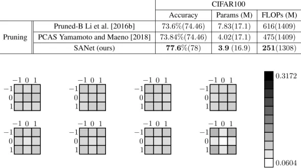
CIFAR100
Accuracy Params (M) FLOPs (M) Pruned-B Li et al. [2016b] 73.6%(74.46) 7.83(17.1) 616(1409) Pruning PCAS Yamamoto and Maeno [2018] 73.84%(74.46) 4.02(17.1) 475(1409) SANet (ours) 77.6%(78) 3.9 (16.9) 251(1308) −1 0 1 −1 0 1 −1 0 1 −1 0 1 −1 0 1 −1 0 1 −1 0 1 −1 0 1 −1 0 1 −1 0 1 −1 0 1 −1 0 1 −1 0 1 −1 0 1 −1 0 1 −1 0 1 0.0604 0.3172
Figure 2: Heat maps representing the average values in A for various layers in the Resnet-20 architecture trained on CIFAR10. In this experiment, values in A are initialized uniformly at random. The first row represents the 4 first layers and the second row the 4 last layers of Resnet-20.
To see how much the initialization of A is related to the distribution of kept weights, we then perform another experiment where A is initialized uniformly at random but then the centre value Ad,c,bS/2c,bS/2cis changed to the maximum over the corresponding slice max(Ad,c,·,·). We observe
in Figure 3 that almost all kept weights in the first layer are slice centres. Subsequent layers yield an almost uniform distribution, and we observe the same kept weights distribution for the last layers as in the previous experiment. We also plot a heat-map of kept weights in Resnet-56 trained on CIFAR10, and where attention tensor A values are initially drawn uniformly at random. Figure 4 shows that for the first layers, the number of kept weights is more important in the centre row than at other positions. However, we see on the last layers that there is more kept weights in the corners than other positions. For further results, we run an experiment in which we replace all 3 × 3 Resnet-20 kernels by 5 × 5 kernels, and train the network on CIFAR10. We observe in Figure 5 that the weights of the center in first layers are more important that other positions. We also see that on the last layers the weight distribution is still not uniform, and the weights on the corners are more important in the last layer. From all these experiments, we consistently observe that in deeper layers, the method tends to keep more weights in corner positions than others, and this independently from initialization process or neural network architecture. This finding interestingly questions the hyperparameters used by the corresponding architectures. It clearly seems the network is more interested in locality in the initial layers than it is in the last layers. Based on this finding, we modified the vanilla shift layer method, using an equivalent uneven distribution of shifts as the one found in our experiments. As such, shifts are predetermined but not uniform. We obtained an accuracy of 94.8% on Resnet-20 and CIFAR10, to be compared to the 93.17% accuracy from Table 1. Interestingly, this accuracy is even better than the results obtained using the method in Jeon and Kim [2018]. On the other hand, the obtained accuracy remains lower than that of the proposed method, suggesting that selecting the shifts during the learning process is still more efficient than having a good choice of predetermined shift proportions.
In a third experiment, we observe the effect of initial and final temperature choices on accuracy. Figure 6: left represents the evolution of accuracy of 20/56 trained on CIFAR10 and
Resnet-−1 0 1 −1 0 1 −1 0 1 −1 0 1 −1 0 1 −1 0 1 −1 0 1 −1 0 1 −1 0 1 −1 0 1 −1 0 1 −1 0 1 −1 0 1 −1 0 1 −1 0 1 −1 0 1 0.0604 0.3172
Figure 3: Heat maps representing the average values in A for various layers in the Resnet-20 architecture trained on CIFAR10. In this experiment, values in A are initialized uniformly at random but the centre value that takes the maximum over the corresponding slice. The first row represents the 4 first layers and the second row the 4 last layers of Resnet-20.
−1 0 1 −1 0 1 −1 0 1 −1 0 1 −1 0 1 −1 0 1 −1 0 1 −1 0 1 −1 0 1 −1 0 1 −1 0 1 −1 0 1 −1 0 1 −1 0 1 −1 0 1 −1 0 1 0.0658 0.1787
Figure 4: Heat maps representing the average values in A for various layers in the Resnet-56 architecture trained on CIFAR10. In this experiment, values in A are initialized uniformly at random. The first row represents the 4 first layers and the second row the 4 last layers of Resnet-56.
0.0258 0.0673 −2 −1 0 1 2 −2 −1 0 1 2 −2 −1 0 1 2 −2 −1 0 1 2 −2 −1 0 1 2 −2 −1 0 1 2 −2 −1 0 1 2 −2 −1 0 1 2 −2 −1 0 1 2 −2 −1 0 1 2 −2 −1 0 1 2 −2 −1 0 1 2 −2 −1 0 1 2 −2 −1 0 1 2 −2 −1 0 1 2 −2 −1 0 1 2
Figure 5: Heat maps representing the average values in A for various layers in the Resnet-20 architecture with 5 × 5 kernels trained on CIFAR10. In this experiment, values in A are initialized uniformly at random. The first row represents the 4 first layers and the second row the 4 last layers.
10−3 10−2 10−1 100 0 50 100 Final temperature Accurac y (%) 10−2 100 102 80 90 Initial temperature Resnet-20+CIFAR10 Resnet56+CIFAR10 Resnet-20+CIFAR100 Resnet-50+CIFAR100
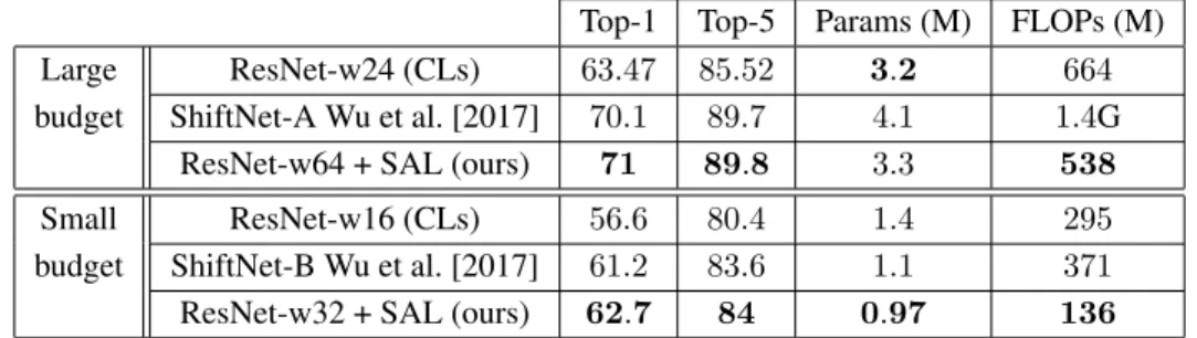
Figure 6: Evolution of accuracy of Resnet-20/56 trained on CIFAR10 and Resnet-20/50 trained on CIFAR100 as function of final temperature (left), and as function of initial temperature (right). Table 4: Comparison of accuracy, number of parameters and FLOPs between a standard CNN, SAL and vanilla Shiftnet on ImageNet ILSVRC 2012.
Top-1 Top-5 Params (M) FLOPs (M) Large ResNet-w24 (CLs) 63.47 85.52 3.2 664 budget ShiftNet-A Wu et al. [2017] 70.1 89.7 4.1 1.4G
ResNet-w64 + SAL (ours) 71 89.8 3.3 538 Small ResNet-w16 (CLs) 56.6 80.4 1.4 295 budget ShiftNet-B Wu et al. [2017] 61.2 83.6 1.1 371 ResNet-w32 + SAL (ours) 62.7 84 0.97 136
20/50 trained on CIFAR100 as function of final temperature while initial temperature is fixed at 6.7. It shows that the accuracy decreases when the final temperature becomes too high. Note that when the final temperature is large, obtained values in A at the end of the training process can be far from binary. In all cases, we round the values in A to the nearest integer before computing the accuracy. This experiment shows that final temperature values need to be small enough so the softmax can push the highest value to 1 and the other values to 0. Figure 6: right shows the behaviour of the accuracy of Resnet-20/56 trained on CIFAR10 and Resnet-20/50 trained on CIFAR100 when initial temperature is changed and final temperature is fixed at 0.02. We see an interesting region between 10 and 6.7 in which the accuracy is better. It is worth mentioning that the choice of initial and final temperature is sensitive with respect to the obtained accuracy. Throughout our experiments, we observed that a too slow decrease in temperature causes the architecture to get stuck in local minima that are poorly fitted to the ending rounding operation. To the contrary, a too fast decrease in temperature prevents the learning procedure from finding the best shifts and boils down to an accuracy that is very similar to that of vanilla shift layers.
In the fourth experiment, we compare the accuracy, memory usage and FLOPs of SAL against vanilla Shiftnet and standard CNN on ImageNet ILSVRC 2012. Table 4 shows that SAL is able to obtain better accuracies than vanilla Shiftnet and standard CNN for the same memory and FLOPs budget.
90 92 94 96 106 2 · 106 4 · 106 Memory footprint T est set accurac y (%) MobileNetV2 SqueezeNet Resnet20 Resnet20+BC Resnet20+BWN Resnet20+SAL Resnet20+SAL2
Figure 7: Evolution of accuracy when applying compression methods on different DNN architectures trained on CIFAR10.
As last experiment, we propose to compare SAL with some other compression methods introduced in Section 3. To get a good approximation of memory needed to implement a neural network on
a limited resources embedded system, we consider both weights and activations when one input data is processed, thus the memory footprint of a DNN will be the memory needed to store both weights and activations. In our evaluation we compare SAL with Binary Connect (BC) Courbariaux et al. [2015] and Binary Weight Network (BWN) Rastegari et al. [2016] applied to Resnet-20, MobileNetV2 Sandler et al. [2018] and Squeezenet Iandola et al. [2016]. We also perform the comparison with another version of SAL denoted SAL2, in which we keep two weights per kernel instead of one. We use Resnet-20 with different number of weights and activations as baseline. Figure 7 shows that the baseline outperforms MobileNetV2, Squeezenet and applying BC on Resnet-20. It also shows that SAL and SAL2 outperform all other methods.
5
Conclusion
In this contribution, we proposed a novel attention-based pruning method that transforms a convo-lutional layer into a shift layer. The resulting network provides interesting improvements in terms of memory and computation time, while keeping high accuracy. Compared to existing methods, we showed that the proposed method results in improved accuracy for similar memory budgets as existing shift-layer based methods, using challenging vision datasets. The proposed method is thus an interesting alternative to channel-pruning methods.
References
Christian Szegedy, Vincent Vanhoucke, Sergey Ioffe, Jon Shlens, and Zbigniew Wojna. Rethinking the inception architecture for computer vision. In Proceedings of the IEEE conference on computer vision and pattern recognition, pages 2818–2826, 2016.
Matthieu Courbariaux, Yoshua Bengio, and Jean-Pierre David. Binaryconnect: Training deep neural networks with binary weights during propagations. In Advances in neural information processing systems, pages 3123–3131, 2015.
Guillaume Soulié, Vincent Gripon, and Maëlys Robert. Compression of deep neural networks on the fly. In International Conference on Artificial Neural Networks, pages 153–160. Springer, 2016. Mohammad Rastegari, Vicente Ordonez, Joseph Redmon, and Ali Farhadi. Xnor-net: Imagenet
classification using binary convolutional neural networks. In European Conference on Computer Vision, pages 525–542. Springer, 2016.
Zhouhan Lin, Matthieu Courbariaux, Roland Memisevic, and Yoshua Bengio. Neural networks with few multiplications. arXiv preprint arXiv:1510.03009, 2015.
Fengfu Li, Bo Zhang, and Bin Liu. Ternary weight networks. arXiv preprint arXiv:1605.04711, 2016a.
Shuchang Zhou, Yuxin Wu, Zekun Ni, Xinyu Zhou, He Wen, and Yuheng Zou. Dorefa-net: Train-ing low bitwidth convolutional neural networks with low bitwidth gradients. arXiv preprint arXiv:1606.06160, 2016.
Song Han, Jeff Pool, John Tran, and William Dally. Learning both weights and connections for efficient neural network. In Advances in neural information processing systems, pages 1135–1143, 2015a.
Junru Wu, Yue Wang, Zhenyu Wu, Zhangyang Wang, Ashok Veeraraghavan, and Yingyan Lin. Deep k-means: Re-training and parameter sharing with harder cluster assignments for compressing deep convolutions. arXiv preprint arXiv:1806.09228, 2018.
Song Han, Huizi Mao, and William J Dally. Deep compression: Compressing deep neural networks with pruning, trained quantization and huffman coding. arXiv preprint arXiv:1510.00149, 2015b. Hao Li, Asim Kadav, Igor Durdanovic, Hanan Samet, and Hans Peter Graf. Pruning filters for
efficient convnets. arXiv preprint arXiv:1608.08710, 2016b.
Arash Ardakani, Carlo Condo, and Warren J Gross. Sparsely-connected neural networks: towards efficient vlsi implementation of deep neural networks. arXiv preprint arXiv:1611.01427, 2016.
François Chollet. Xception: Deep learning with depthwise separable convolutions. arXiv preprint, pages 1610–02357, 2017.
Andrew G Howard, Menglong Zhu, Bo Chen, Dmitry Kalenichenko, Weijun Wang, Tobias Weyand, Marco Andreetto, and Hartwig Adam. Mobilenets: Efficient convolutional neural networks for mobile vision applications. arXiv preprint arXiv:1704.04861, 2017.
Mark Sandler, Andrew Howard, Menglong Zhu, Andrey Zhmoginov, and Liang-Chieh Chen. Mo-bilenetv2: Inverted residuals and linear bottlenecks. In Proceedings of the IEEE Conference on Computer Vision and Pattern Recognition, pages 4510–4520, 2018.
Quanshi Zhang, Ying Nian Wu, and Song-Chun Zhu. Interpretable convolutional neural networks. In Proceedings of the IEEE Conference on Computer Vision and Pattern Recognition, pages 8827–8836, 2018.
Felix Juefei-Xu, Vishnu Naresh Boddeti, and Marios Savvides. Local binary convolutional neural networks. In 2017 IEEE Conference on Computer Vision and Pattern Recognition (CVPR), pages 4284–4293. IEEE, 2017.
Christian Szegedy, Vincent Vanhoucke, Sergey Ioffe, Jonathon Shlens, and Zbigniew Wojna. Re-thinking the inception architecture for computer vision. arXiv preprint arXiv:1512.00567, 2015. Karen Simonyan and Andrew Zisserman. Very deep convolutional networks for large-scale image
recognition. arXiv preprint arXiv:1409.1556, 2014.
Forrest N Iandola, Song Han, Matthew W Moskewicz, Khalid Ashraf, William J Dally, and Kurt Keutzer. Squeezenet: Alexnet-level accuracy with 50x fewer parameters and < 0.5 mb model size. arXiv preprint arXiv:1602.07360, 2016.
Bichen Wu, Alvin Wan, Xiangyu Yue, Peter Jin, Sicheng Zhao, Noah Golmant, Amir Gholaminejad, Joseph Gonzalez, and Kurt Keutzer. Shift: A zero flop, zero parameter alternative to spatial convolutions. arXiv preprint arXiv:1711.08141, 2017.
Ghouthi Boukli Hacene, Vincent Gripon, Matthieu Arzel, Nicolas Farrugia, and Yoshua Bengio. Quantized guided pruning for efficient hardware implementations of convolutional neural networks. arXiv preprint arXiv:1812.11337, 2018.
Yifan Yang, Qijing Huang, Bichen Wu, Tianjun Zhang, Liang Ma, Giulio Gambardella, Michaela Blott, Luciano Lavagno, Kees Vissers, John Wawrzynek, et al. Synetgy: Algorithm-hardware co-design for convnet accelerators on embedded fpgas. arXiv preprint arXiv:1811.08634, 2018. Ashish Vaswani, Noam Shazeer, Niki Parmar, Jakob Uszkoreit, Llion Jones, Aidan N Gomez, Łukasz
Kaiser, and Illia Polosukhin. Attention is all you need. In Advances in Neural Information Processing Systems, pages 5998–6008, 2017.
Matthieu Courbariaux, Itay Hubara, Daniel Soudry, Ran El-Yaniv, and Yoshua Bengio. Binarized neural networks: Training deep neural networks with weights and activations constrained to+ 1 or-1. arXiv preprint arXiv:1602.02830, 2016.
Karen Ullrich, Edward Meeds, and Max Welling. Soft weight-sharing for neural network compression. arXiv preprint arXiv:1702.04008, 2017.
Yang He, Guoliang Kang, Xuanyi Dong, Yanwei Fu, and Yi Yang. Soft filter pruning for accelerating deep convolutional neural networks. arXiv preprint arXiv:1808.06866, 2018.
Ruichi Yu, Ang Li, Chun-Fu Chen, Jui-Hsin Lai, Vlad I Morariu, Xintong Han, Mingfei Gao, Ching-Yung Lin, and Larry S Davis. Nisp: Pruning networks using neuron importance score propagation. In Proceedings of the IEEE Conference on Computer Vision and Pattern Recognition, pages 9194–9203, 2018.
Qiangui Huang, Kevin Zhou, Suya You, and Ulrich Neumann. Learning to prune filters in convolu-tional neural networks. arXiv preprint arXiv:1801.07365, 2018.
Kohei Yamamoto and Kurato Maeno. Pcas: Pruning channels with attention statistics. arXiv preprint arXiv:1806.05382, 2018.
Yunho Jeon and Junmo Kim. Constructing fast network through deconstruction of convolution. arXiv preprint arXiv:1806.07370, 2018.
Kaiming He, Xiangyu Zhang, Shaoqing Ren, and Jian Sun. Identity mappings in deep residual networks. In European conference on computer vision, pages 630–645. Springer, 2016.
Alex Krizhevsky, Ilya Sutskever, and Geoffrey E Hinton. Imagenet classification with deep convolu-tional neural networks. In Advances in neural information processing systems, pages 1097–1105, 2012.