Polarization properties of a sample of broad absorption line and gravitationally lensed quasars

AND

ASTROPHYSICS

Polarization properties of a sample of broad absorption line

and gravitationally lensed quasars

?,??

D. Hutsem´ekers???, H. Lamy, and M. Remy

Institut d’Astrophysique, Universit´e de Li`ege, 5 av. de Cointe, B-4000 Li`ege, Belgium Received 20 July 1998 / Accepted 29 September 1998

Abstract. New broad-band linear polarization measurements have been obtained for a sample of 42 optically selected QSOs including 29 broad absorption line (BAL) QSOs. The polariza-tion properties of different sub-classes have been compared, and possible correlations with various spectral indices searched for. The main results of our study are: (1) Nearly all highly po-larized QSOs of our sample belong to the sub-class of BAL QSOs with low-ionization absorption features (LIBAL QSOs). (2) The range of polarization is significantly larger for LIBAL QSOs than for high-ionization (HI) BAL QSOs and non-BAL QSOs. (3) There is some indication that HIBAL QSOs as a class may be more polarized than non-BAL QSOs and therefore inter-mediate between LIBAL and non-BAL QSOs, but the statistics are not compelling from the sample surveyed thus far. (4) For LIBAL QSOs, the continuum polarization appears significantly correlated with the line profile detachment index, in the sense that LIBAL QSOs with P Cygni-type profiles are more polar-ized. No correlation was found with the strength of the low- or the high-ionization absorption features, nor with the strength or the width of the emission lines.

These results are consistent with a scenario in which LIBAL QSOs constitute a different class of radio-quiet QSOs with more absorbing material and more dust. Higher maximum polarization can therefore be reached, while the actually measured polarization depends on the geometry and orientation of the system as do the line profiles. The observed correlation is interpreted within the framework of recent “wind-from-disk” models.

Key words: polarization – galaxies: quasars: absorption lines – galaxies: quasars: general – cosmology: gravitational lensing

? _{Tables 2 and 3 are also available in electronic form at the}

CDS via anonymous ftp to cdsarc.u-strasbg.fr (130.79.128.5) or via http://cdsweb.u-strasbg.fr/Abstract.html

??

Based on observations collected at the European Southern Obser-vatory (ESO, La Silla)

??? _{Also, Chercheur Qualifi´e au Fonds National de la Recherche}

Sci-entifique (FNRS, Belgium)

1. Introduction

Broad absorption line quasi-stellar objects (BAL QSOs) are characterized by the presence in their spectra of broad, often deep, absorption troughs in the resonance lines of highly-ionized species like Civ, Si iv, or N v. These BALs appear blueshifted

with respect to the corresponding emission lines. They are gen-erally attributed to the ejection of matter at very high velocities (∼0.1 c). About 12% of optically selected QSOs have BALs

in their spectra, although this fraction could be underestimated if at least some BAL QSOs have their continuum more attenu-ated than non-BAL QSOs (Goodrich 1997). Apparently all BAL QSOs are radio-quiet1(Stocke et al. 1992). A recent account of BAL QSO properties may be found in Arav et al. (1997).

The fact that the broad emission line properties are essen-tially similar for BAL and non-BAL QSOs suggests that all radio-quiet QSOs could have a BAL region (BALR) of small covering factor, the BAL QSOs themselves being those objects with the BALR along the line of sight (e.g. Weymann et al. 1991, hereafter WMFH). Alternately, BAL and non-BAL QSOs may constitute two physically distinct populations of objects, BAL QSOs possibly representing an early stage in an evolutionary process towards normal QSOs (e.g. Boroson & Meyers 1992). As first noticed by Stockman, Moore & Angel (1984), a number of BAL QSOs show high optical polarization (≥ 3%)

in the continuum while other radio-quiet QSOs (i.e. non-BAL ones) have generally low polarization (≤ 1%). This important

result has been recently confirmed by Hines & Schmidt (1997) on the basis of a larger sample. The fact that there is little or no variability of the polarization clearly distinguishes BAL QSOs from the so-called blazars. Since polarization is sensitive to the geometry of the objects (without spatially resolving them), a detailed understanding of BAL QSO polarization properties may provide important clues on the nature of the outflows and the status of these objects among AGN.

In this view, we have started a systematic polarimetric study of BAL QSOs. The present paper is devoted to the analysis of new broad-band polarization measurements obtained for a

sam-1

There is only one known candidate radio-loud BAL QSO, 1556+3517, recently discovered by Becker et al. (1997). But Clavel (1998) finds that its radio-loudness is marginal after correcting for red-dening

ple of 29 BAL QSOs, to which a number of normal radio-quiet QSOs have been added for comparison. Since an important issue is the study of possible correlations between polarization and other spectral characteristics, the objects have been essentially picked out from the WMFH sample which provides many useful quantitative spectral indices. Further, at least one BAL QSO is known to be gravitationally lensed. Its polarization could then be affected or induced by microlensing effects, i.e. by the selec-tive magnification of some regions. We have therefore added to our sample several gravitationally lensed non-BAL QSOs with the aim of detecting any possible polarization difference.

The paper is organized as follows: the observing strategy and techniques are described in Sect. 2, as well as the methods for reducing the data and extracting accurate measurements. Instrumental polarization and de-biasing are also discussed in this section. In Sect. 3, the final sample of observed objects is detailed, sub-classes are defined, and several quantities char-acterizing the optical spectra are presented. Results are given in Sect. 4, including correlation searches between the various quantities. Conclusions and discussion form the last section.

2. Polarimetric observations and data reduction

The polarimetric observations were carried out on March 14–17 and September 3–6, 1994, at the European Southern Observa-tory (ESO La Silla, Chile), using the 3.6m telescope equipped with the EFOSC1 camera and spectrograph. The detector was a 512×512 TeK CCD (ESO#26) with a pixel size of 27 µm

corresponding to 000._{605 on the sky.}

With EFOSC1, polarimetry is performed by inserting in the parallel beam a Wollaston prism which splits the incoming light rays into two orthogonally polarized beams. Each object in the field has therefore two images on the CCD detector, separated by about 2000_{and orthogonally polarized. To avoid image} over-lapping, one puts at the telescope focal plane a special mask made of alternating transparent and opaque parallel strips whose width corresponds to the splitting. The object is positioned at the centre of a transparent strip which is imaged on a region of the CCD chosen as clean as possible. The final CCD image then consists of alternate orthogonally polarized strips of the sky, two of them containing the polarized images of the object itself (Melnick et al. 1989, di Serego Alighieri 1989).

In order to derive linear polarization measurements, i.e. the two normalized Stokes parametersq and u, frames must be

ob-tained with at least two different orientations of the Wollaston prism. This was done by rotating the whole EFOSC1 instru-ment by 45◦_{(usually at the adapter angles 270}◦_{and 225}◦_{). For} each object, two frames are therefore obtained. Typical expo-sure times are around 600s per frame, generally split into two shorter exposures. All observations were done with the Bessel V filter (ESO#553). The seeing was typically between 100_and 200_{, and the nights were photometric most of the time. Note that} the polarization measurements do not depend on variable trans-parency or seeing since the two orthogonally polarized images of the object are simultaneously recorded. Finally, polarimet-ric calibration stars were observed (HD90177, HD161291, and

HD164740; Schwarz 1987) in order to unambiguously fix the zero-point of the polarization position angle and to check the whole observing and reduction process.

Considering the two frames obtained with the instrument rotated at 270◦_{and 225}◦_{, the normalized Stokes parameters are} given by q = I 1 270− I 2 270 I1 270+ I 2 270 , u = I 1 225− I 2 225 I1 225+ I 2 225 , (1) whereI1 andI2

respectively refer to the intensities integrated over the two orthogonally polarized images of the object, back-ground subtracted (Melnick et al. 1989). At this stage, the sign of

q and u is arbitrary. It is clear from these relations that intensities

must be determined with the highest accuracy. For this, the data were first corrected for bias and dark emission, and flat-fielded. A plane was locally fitted to the sky around each object image, and subtracted from each image individually. Since it appeared that standard aperture photometry was not accurate enough due to the rather large pixel size, we have measured the object center at subpixel precision by fitting a 2D gaussian profile and inte-grated the flux in a circle of same center and arbitrary radius by taking into account only those fractions of pixels inside the circle. With this method, the Stokes parameters may be com-puted for any reasonable radius of the aperture circle. They were found to be stable against radius variation, giving confidence in the method. In order to take as much flux as possible with not too much sky background, we finally fixed the aperture radius at 2.5(2 ln 2)−1/2_{HW, where HW is the mean width at} half-maximum of the gaussian profile. Note that in the few cases where the objects are resolved into multiple components, we use the smallest square aperture encompassing all the compo-nents. The whole procedure has been implemented within the ESO MIDAS reduction package. Applied to calibration stars, it provides polarization measurements in good agreement with the tabulated values. The zero-point of the polarization position angle is also determined from these stars, and the sign ofq and u

accordingly fixed. The uncertaintiesσqandσuare evaluated by computing the errors on the intensitiesI1

andI2

from the read-out noise and from the photon noise in the object and the sky background (after converting the counts in electrons), and then by propagating these errors in Eq. 1. Uncertainties are typically around 0.15% for bothq and u.

Since on most CCD frames field stars are simultaneously recorded, one can in principle use them to estimate the instru-mental polarization, and to correct frame-by-frame the quasar Stokes parameters, following a method described by di Serego Alighieri (1989). However, the field stars (even when combined in a single “big” one per frame) are often fainter than the quasar, and a frame-by-frame correction introduces uncertainties on the quasar polarization larger than the instrumental polarization it-self. Therefore, we tried to empirically correlate the instrumen-tal polarization with observational parameters like the observ-ing time or the position of the telescope, in order to check for possible variation and/or to derive a useful relation. Since no significant variation was found, we have finally computed the weighted average and dispersion of the normalized Stokes

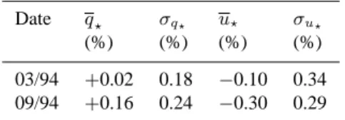
pa-Table 1. Instrumental polarization

Date q_? σq? u? σu?

(%) (%) (%) (%)

03/94 +0.02 0.18 −0.10 0.34 09/94 +0.16 0.24 −0.30 0.29

rameters of field stars (a single “big” one per frame) considering all frames obtained during a given run. These values are given in Table 1. They indicate that the instrumental polarization is small. We take it into account in a rather conservative way by subtract-ing the systematicq? andu? from the quasarq and u, and by adding quadratically the errors. The final, corrected, values of the normalized Stokes parametersq and u are given in Table 2,

together with the uncertainties. Note that possible contamina-tion by interstellar polarizacontamina-tion is included in the uncertainties (see also Sect. 4.1).

Then, from these values, the polarization degree is evalu-ated with p = (q2

+ u2

)1/2_{, while the polarization position} angleθ is obtained by solving the equations q = p cos 2θ and u = p sin 2θ. The error on the polarization degree is estimated

byσp = (σq+ σu)/2, although the complex statistical behavior of the polarization degree should be kept in mind (Serkowski 1962, Simmons & Stewart 1985). Indeed, sincep is always a

positive quantity, it is biased at low signal-to-noise ratio. A rea-sonably good estimator of the true polarization degree, notedp0, is computed fromp and σpusing the Wardle & Kronberg (1974) method (Simmons & Stewart 1985). Finally, the uncertainty of the polarization position angleθ is estimated from the standard

Serkowski (1962) formula wherep0is used instead ofp to avoid biasing, i.e.σθ = 28.◦65 σp/p0. All these quantities are given in Table 2. Also reported are the redshiftz of the objects, the

quasar sub-type (cf. Sect. 3.1), andpISM, an upper limit to the

galactic interstellar polarization along the object line of sight (cf. Sect. 4.1)

3. The observed sample and its characteristics

The observed QSOs were essentially chosen from the WMFH sample, which is a set of BAL and non-BAL QSOs from the Large Bright Quasar Survey (LBQS, cf. Hewett et al. 1995), augmented by several BAL QSOs from other sources. The se-lection was achieved during the observations depending on the QSO observability (position on the sky) and magnitude (priority to the brighter objects). A priority was also given to the BAL QSOs with low-ionization features. Five objects observable in the southern sky were added: 3 BAL QSOs from the Hartig & Baldwin (1986, hereafter HB) sample (0254-3327, 0333-3801, 2240-3702), and 2 non-BAL QSOs from the LBQS (2114-4346, 2122-4231). Finally, an additional 7 true or possible gravita-tionally lensed optically selected QSOs (cf. the compilation by Refsdal & Surdej 1994) were included in the sample.

The final sample then consists of 42 moderate to high red-shift optically selected QSOs (cf. Tables 2 & 3). It contains 29 BAL QSOs, 12 non-BAL QSOs, and 1 “intermediate” object

(2211-1915, cf. WMFH). 8 of them are true or possible gravita-tionally lensed QSOs, including 2 BAL QSOs: 1413+1143 and 1120+01542_.

Among the 42 optically selected QSOs, 36 are definitely radio-quiet while only 1 is radio-loud (2211-1915, the “inter-mediate” object) (Stocke et al. 1992, Hooper et al. 1995, V´eron & V´eron 1996, Djorgovski & Meylan 1989, Bechtold et al. 1994, Reimers et al. 1995). The 5 remaining objects (3 BAL QSOs and 2 non-BAL QSOs: 0333-3801, 0335-3339, 2154-2005, 2114-4346, 2122-4231) have apparently not been mea-sured at radio-wavelengths. However, they are most probably radio-quiet too (Stocke et al. 1992, Hooper et al. 1995).

3.1. The low-ionization BAL QSOs

Approximately 15% of BAL QSOs have deep low-ionization BALs (Mgii λ 2800 and/or Al iii λ 1860) in addition to the usual

high-ionization BAL troughs (WMFH, Voit et al. 1993). These objects might be significantly reddened by dust (Sprayberry & Foltz 1992). They also possibly constitute a physically different class of BAL QSOs (Boroson & Meyers 1992).

While objects with strong low-ionization (LI) features are recognized as LIBAL QSOs by most authors, the classification of objects with weaker features is controversial. We therefore define three categories of LIBAL QSOs: strong (S), weak (W), and marginal (M) LIBAL QSOs. The strong and weak LIBAL QSOs in our sample were all considered and first classified as such by WMFH. The strong ones are 0059-2735, 1011+0906, 1232+1325 and 1331-0108; the weak ones are 0335-3339, 1231+1320, 2225-0534 and 2350-0045 (WMFH “a” parame-ter< 1). But the classification by WMFH is rather conservative

and includes only clear LIBAL QSOs, while several authors have reported faint LIBAL features in a number of other objects. We classify the latter objects as marginal LIBAL QSOs. These are 0043+0048, 1246-0542 and 2240-3702 (HB), 1413+1143 (Hazard et al. 1984, Angonin et al. 1990), 1120+0154 (Meylan & Djorgovski 1989), and 1212+1445 (this work). The marginal LIBAL QSOs are characterized by very weak Mgii and/or Al iii

BALs. The asymmetry of the Mgii or C iii] emission lines,

when cut on the blue side, is also considered as evidence for marginal LIBALs. Note finally that line strengths may be vari-able in some objects and that weak LIBALs could have been observed only once (namely due to possible microlensing ef-fects as suspected in e.g. 1413+1143; Angonin et al. 1990, Hut-sem´ekers 1993).

The remaining BAL QSOs are classified as high ionization (HI) only, except 0903+1734 and 1235+0857 which are unclas-sified, the Mgii line being outside the observed spectral range

and no Aliii BAL being detected. These classifications are

sum-marized in Tables 2 and 3. Note that most spectra available in the literature were carefully re-inspected to check for the con-sistency of the classification. Altogether, the strong, weak and marginal LIBAL QSOs constitute approximately 50% of our

2 _{Note that 1120+0154 = UM425 was only recently recognized as a}

Table 2. Polarimetric results

Object z Type q σq u σu p σp p0 pISM θ σθ

(%) (%) (%) (%) (%) (%) (%) (%) (◦_{) (}◦₎ 0006+0230 2.096 10 0.04 0.27 −0.10 0.31 0.11 0.29 0.00 0.08 145 – 0013−0029 2.084 10 −0.65 0.30 −0.79 0.35 1.03 0.33 0.97 0.07 115 10 0019+0107 2.124 20 0.13 0.27 0.88 0.30 0.89 0.29 0.85 0.10 41 10 0021−0213 2.296 20 0.65 0.30 −0.25 0.34 0.70 0.32 0.63 0.17 170 14 0025−0151 2.072 20 −0.37 0.26 0.24 0.31 0.44 0.28 0.37 0.15 74 22 0029+0017 2.226 20 0.54 0.32 −0.52 0.35 0.75 0.34 0.68 0.10 158 14 0043+0048 2.141 50 −0.14 0.27 −0.07 0.31 0.16 0.29 0.00 0.02 103 – 0059−2735 1.594 30 1.56 0.26 −0.44 0.31 1.62 0.29 1.60 0.16 172 5 0137−0153 2.232 20 −0.61 0.27 0.94 0.31 1.12 0.29 1.08 0.08 61 8 0142−1000 2.719 11 0.00 0.29 −0.28 0.33 0.28 0.31 0.00 0.08 135 – 0145+0416 2.029 20 −0.42 0.30 −2.67 0.34 2.70 0.32 2.68 0.21 131 3 0254−3327 1.862 20 −0.20 0.36 −0.02 0.40 0.20 0.38 0.00 0.04 93 – 0333−3801 2.210 20 0.01 0.26 0.83 0.30 0.83 0.28 0.78 0.00 45 10 0335−3339 2.258 40 0.02 0.33 0.60 0.35 0.60 0.34 0.53 0.00 44 19 0903+1734 2.776 60 −0.47 0.21 0.80 0.36 0.93 0.29 0.88 0.12 60 9 1009−0252 2.745 11 0.94 0.22 −0.07 0.38 0.95 0.30 0.90 0.07 178 9 1011+0906 2.262 30 0.60 0.23 −2.04 0.37 2.12 0.30 2.10 0.06 143 4 1029−0125 2.038 20 −0.54 0.24 −0.99 0.38 1.13 0.31 1.09 0.21 121 8 1104−1805 2.303 11 0.18 0.20 0.24 0.35 0.30 0.27 0.17 0.27 27 45 1115+0802 1.722 11 −0.02 0.19 0.68 0.35 0.68 0.27 0.63 0.17 46 12 1120+0154 1.465 51 1.84 0.19 0.63 0.35 1.95 0.27 1.93 0.17 9 4 1146+0207 2.055 10 0.22 0.25 −0.42 0.39 0.47 0.32 0.39 0.08 149 23 1208+1011 3.803 11 −0.18 0.24 0.30 0.37 0.35 0.30 0.23 0.00 60 38 1208+1535 1.956 20 −0.17 0.36 −0.11 0.47 0.20 0.42 0.00 0.28 107 – 1212+1445 1.621 50 0.98 0.23 1.06 0.36 1.45 0.30 1.42 0.25 24 6 1231+1320 2.386 40 0.59 0.25 −0.45 0.39 0.74 0.32 0.68 0.10 162 14 1232+1325 2.363 30 −1.95 0.30 −0.53 0.40 2.02 0.35 1.99 0.11 98 5 1235+0857 2.885 60 1.68 0.22 1.55 0.37 2.29 0.29 2.27 0.00 21 4 1246−0542 2.222 50 0.35 0.20 −0.84 0.36 0.91 0.28 0.87 0.07 146 9 1309−0536 2.212 20 0.78 0.21 −0.03 0.36 0.78 0.28 0.73 0.13 179 11 1331−0108 1.867 30 1.01 0.27 1.59 0.35 1.88 0.31 1.86 0.09 29 5 1413+1143 2.542 51 −0.78 0.25 1.32 0.36 1.53 0.31 1.50 0.00 60 6 1429−0053 2.084 11 0.95 0.18 0.31 0.40 1.00 0.29 0.96 0.18 9 9 1442−0011 2.215 20 0.16 0.22 −0.18 0.37 0.24 0.30 0.00 0.25 156 – 2114−4346 2.041 10 −0.11 0.29 −0.22 0.34 0.24 0.31 0.00 0.15 122 – 2122−4231 2.266 10 −0.01 0.27 −0.12 0.31 0.12 0.29 0.00 0.17 133 – 2154−2005 2.028 20 0.26 0.26 −0.70 0.30 0.75 0.28 0.69 0.07 145 12 2211−1915 1.951 10 0.14 0.27 0.03 0.31 0.14 0.29 0.00 0.08 6 – 2225−0534 1.981 40 3.58 0.27 −2.51 0.31 4.37 0.29 4.36 0.33 162 2 2230+0232 2.147 10 −0.36 0.28 −0.57 0.31 0.68 0.29 0.62 0.38 119 14 2240−3702 1.835 50 0.92 0.26 1.88 0.30 2.10 0.28 2.08 0.00 32 4 2350−0045 1.626 40 −0.58 0.27 −0.16 0.31 0.60 0.29 0.53 0.24 98 16

Object Type: First digit: (1) non-BAL QSOs + one intermediate object, (2) HIBAL QSOs, (3) Strong LIBAL QSOs, (4) Weak LIBAL QSOs, (5) Marginal LIBAL QSOs, (6) unclassified BAL QSOs; Second digit: (1) objects identified as true or possible gravitationally lensed QSOs

BAL QSO sample (but this is not representative of the actual proportion of LIBAL QSOs among BAL QSOs since priority was given to these objects).

3.2. The BAL QSO spectral characteristics

WMFH provide a series of spectral indices characterizing the absorption and emission features of BAL QSOs. For the absorp-tion lines, they define the balnicity index (BI, in km s−1_{) which}

is a modified velocity equivalent width of the Civ BAL, and

the detachment index (DI, unitless) which measures the onset velocity of the strongest Civ BAL trough in units of the

adja-cent emission line half-width, that is, the degree of detachment of the absorption line relative to the emission one (see also HB who first distinguish between detached and P Cygni-type BAL profiles). Estimates of BI are also given by Korista et al. (1993) for most objects of our sample, such that we adopt for BI an average of these values and those from WMFH. WMFH also

Table 3. BAL QSO spectral characteristics

Object Type BI DI Civ Ciii] Civ Ciii] Feii 2400 Feii 2070 αB αR

HW HW EW EW EW EW 0019+0107 20 2305 4.65 1432 4193 7.5 18.1 21.99 5.96 0.73 0.68 0021−0213 20 5180 3.14 3077 3856 7.7 17.2 46.74 3.56 0.66 0.68 0025−0151 20 2878 2.97 1645 2528 10.9 23.4 19.90 1.96 0.34 1.07 0029+0017 20 5263 2.45 1857 3219 15.1 31.7 27.34 4.99 0.55 1.13 0043+0048 50 4452 10.06 987 1586 2.8 12.5 44.66 4.80 −0.13 0.77 0059−2735 30 11054 1.18 – – – – 40.91 8.36 1.50 1.59 0137−0153 20 4166 2.41 1935 3125 8.2 22.6 35.95 6.32 1.01 1.26 0145+0416 20 4765 3.96 2341 – 12.5 – 33.10 5.36 0.96 0.42 0254−3327 20 694 1.08 1640 3125 8.1 22.5 23.00 2.40 0.64 0.91 0333−3801 20 3432 3.28 5450 3063 7.5 6.3 37.00 6.60 0.56 0.07 0335−3339 40 7460 15.90 599 – 1.7 – 95.66 14.16 1.91 1.74 0903+1734 60 9776 4.34 1548 5630 4.7 26.5 – 4.90 1.54 0.59 1011+0906 30 5587 6.84 3232 3754 7.9 11.1 40.91 9.16 1.95 1.51 1029−0125 20 1849 2.22 1645 3400 8.0 23.2 42.96 4.41 0.83 1.47 1120+0154 51 415 0.79 1343 – 8.5 – – – 0.45 1.25 1208+1535 20 4545 4.64 2709 5222 6.3 24.0 23.98 6.92 0.42 1.06 1212+1445 50 3619 6.05 1741 2363 3.8 4.9 25.29 3.37 1.51 1.08 1231+1320 40 3473 6.38 2612 4492 7.5 18.6 42.59 7.19 2.15 0.22 1232+1325 30 12620 1.84 3870 7123 17.5 42.9 58.76 11.80 2.38 0.92 1235+0857 60 815 0.42 1296 3840 10.4 24.0 – 3.00 1.04 0.45 1246−0542 50 4309 6.60 1587 3699 4.8 20.1 44.29 4.21 1.84 0.88 1309−0536 20 5363 5.10 3812 5128 8.1 23.7 36.42 5.19 1.41 0.90 1331−0108 30 7912 1.15 1935 3212 6.2 13.8 18.07 6.95 2.66 1.62 1413+1143 51 6621 1.50 1683 2937 18.8 35.0 – 1.89 1.72 0.63 1442−0011 20 5143 2.83 3522 5481 14.6 20.0 25.81 4.12 0.58 1.16 2154−2005 20 963 6.42 2438 3392 11.3 26.9 21.91 4.47 0.41 0.62 2225−0534 40 7903 0.48 1509 3251 11.3 43.4 53.38 7.67 1.68 2.21 2240−3702 50 8539 0.69 1940 3000 7.7 16.2 – 3.80 1.08 1.40 2350−0045 40 6964 5.08 1761 – 14.3 – 54.78 5.71 1.01 1.03

Object Type: First digit: (2) HIBAL QSOs, (3) Strong LIBAL QSOs, (4) Weak LIBAL QSOs, (5) Marginal LIBAL QSOs, (6) unclassified BAL QSOs; Second digit: (1) objects identified as true or possible gravitationally lensed QSOs. Units are given in the text

provide “clever” half-widths at half-maximum (HW, in km s−1₎ and equivalent widths (EW, in ˚A) for the Civ, C iii] and Fe ii

emission lines. For a more detailed definition of these indices, see WMFH.

For a few objects (0254-3327, 0333-3801, 2240-3702, and 1120+0154), some spectral indices were not provided. We there-fore computed them using Civ spectra published by Korista et

al. (1993) and Steidel & Sargent (1992). The spectra were dig-itally scanned, and the measurements done following the pre-scriptions given by WMFH. The measurements were also done for spectra of objects with published indices: a good agreement was found, giving confidence in our new values. For the Ciii]

and Feii emission lines, half-widths and equivalent widths were

simply rescaled from those measured by HB. All these quanti-ties are reported in Table 3.

In addition, we have evaluated the slope of the continuum using BAL QSO spectra digitally scanned from the papers by WMFH, HB, and Steidel & Sargent (1992). After some trials, we realized that some spectra cannot be easily fitted with a sin-gle power-law continuum: the slope often breaks roughly near Ciii], probably due to reddening and/or extended Fe ii emission

(compare for example the spectra of 1246-0542 and 1442-0011 in WMFH). We therefore decided to fit the continuum blue-ward and redblue-ward of Ciii], independently. The derived slopes αBandαRare given in Table 3, assuming a power-law

contin-uumFν ∝ ν−α. The values ofαBandαRare affected by large

uncertainties (not smaller than∆α ∼ 0.3), mainly due to the

difficulty to accurately identify the continuum when the BALs are very large, when the Feii emission/absorption is strong, or

when the Mgii absorption is wide.

4. The results

4.1. Contamination by interstellar polarization

Since all objects in the sample are at high galactic latitudes (|bII| > 35◦), the contamination by interstellar polarization in

the Galaxy is expected to be negligible. This may be verified using the Burstein & Heiles (1982, hereafter BH) reddening maps3_{. The maps provide E(B-V) values from which the}

inter-3 _{The data files and routines were obtained from Schlegel 1998, via}

Fig. 1. The QSO polarization degree p0 (in%)

[ut] is represented here as a function of the

Galac-tic latitude of the objects (|bII|, in degree),

to-gether with the de-biased polarization degree of field stars [×] (also corrected for the small

systematic trend reported in Table 1), and the maximum interstellar polarization degree pISM

derived from the Burstein & Heiles (1982) red-dening maps [+]

stellar polarization is estimated with the relationpISM ≤ 8.3%

E(B-V) (Hiltner 1956). These upper limits onpISMare reported

in Table 2. All but two are smaller than 0.3%, indicating a very small contamination by the Galaxy.

Polarization of faint field stars recorded on the CCD frames may also provide an estimate of the interstellar polarization. The dispersion of their Stokes parameters (Table 1) indicates that actually both instrumental and interstellar polarization are small. This is further illustrated in Fig. 1, where the QSO po-larization is compared to the field star popo-larization (interstellar + instrumental), and to the maximum interstellar polarization derived from the BH maps. The absence of correlation between the field star polarization and the BH interstellar polarization suggests that instrumental polarization dominates field star po-larization (although one cannot exclude that a few of them are intrinsically polarized). In addition, no deviation from unifor-mity was found in the distribution of the acute angle between quasar and field star polarization vectors measured on the same frame. These results confirm the insignificance of interstellar polarization in our sample.

We may therefore safely conclude that virtually any quasar withp0 ≥ 0.5% (or p ≥ 0.6%) is intrinsically polarized (cf. Fig. 1 and Table 1), in good agreement with the results obtained by Berriman et al. (1990) for low-polarization Palomar-Green (PG) QSOs.

4.2. Polarization variability

For some BAL QSOs of our sample, previous polarimetric mea-surements are available in the literature, and may be used for comparison. In Table 4, we list first epoch measurements ob-tained in 1977–1981. For all these objects, and within the limits of uncertainty, the values of the polarization position angles are in excellent agreement with ours (Table 2).

Table 4. Previous polarimetric measurements

Object Date p σp θ σθ (%) (%) (◦_{) (}◦₎ 0019+0107 11-05-78 0.93 0.26 24 8 0043+0048 11-05-78 0.33 0.38 103 25 0145+0416 10-23-81 0.58 0.68 131 34 0254−3327 10-24-81 0.62 1.16 154 54 1246−0542 4-05-78 1.87 0.31 139 5 1309−0536 6-09-78 2.33 0.57 179 7 1413+1143 6-06-81 3.39 0.48 49 4 2225−0534 9-11-77 4.09 0.79 166 6

From Moore & Stockman 1981, 1984, and Stockman et al. 1984

On the contrary, our values ofp are generally smaller than

or equal to the previous ones. However variability cannot be invoked since the observed differences are most likely due to the fact that the old measurements were done in white light and using detectors more sensitive in the blue, i.e. in a wavelength range where polarization is suspected to be higher (cf. Stockman et al. 1984, and more particularly the case of 1246-0542). Note further that those objects with null polarization (p ≤ σp) are identical, except 0145+0416 which we find significantly polar-ized. But 0145+0416 is also the only object in our sample not far from a bright star which might contaminate the measurements. Its variability can nevertheless not be excluded.

In conclusion, we find no evidence in our sample of BAL QSOs for the strong polarization variability (in degree or angle) which characterizes blazars, confirming on a larger time-scale the results of Moore & Stockman (1981). This does not preclude the existence of small variations like those reported by Goodrich & Miller (1995) for 1413+1143.

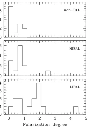
Fig. 2. The distribution of the polarization degree p0(in%) for the three

main classes of QSOs. Non-BAL QSOs include the intermediate object. LIBAL QSOs contain the three sub-categories, i.e. strong, weak and marginal LIBAL QSOs

4.3. Polarization versus QSO sub-types

Before discussing the polarization properties of the different QSO sub-types, it is important to note that our sample is quite ho-mogeneous in redshift (as from WMFH). Therefore, the polar-ization we measure in the V filter roughly refers to the same rest-frame wavelength range, such that differences between quasar sub-types will not be exaggerately masked by a possible wave-length dependence of the polarization. Also, spectral lines gen-erally contribute little to the total flux in the V filter, and our polarimetric measurements largely refer to the polarization in the continuum.

Fig. 2 illustrates the distribution of p0 for non-BAL, HI-BAL and LIHI-BAL QSOs. It immediately appears that nearly all QSOs with high polarization (p0 ≥ 1.2%) are LIBAL QSOs. Only two other objects have high polarization (cf. Table 2): 1235+0857 which is unclassified (and therefore could be a LIBAL QSO), and 0145+0416 which has uncertain measure-ments (cf. Sect. 4.2). Also important is the fact that not all LIBAL QSOs do have high polarization (like 0335-3339 or 1231+1320 which are bona-fide ones; cf. WMFH and Voit et al. 1993). Further, although the strongest LIBAL QSOs are all highly polarized, there is apparently no correlation between the LIBAL strength and the polarization degree (cf. 2225-0534 or 1120+0154 which are weak and marginal LIBAL QSOs, re-spectively). This suggests that polarization is not systematically higher in LIBAL QSOs, but that its range is wider than in other

Table 5. Comparison of p0for various pairs of samples

Sample 1 Sample 2 n1 n2 PK₋S non-BAL BAL 13 29 0.0253 non-BAL LIBAL 13 14 0.0076 non-BAL HIBAL 13 13 0.2914 non-BAL HIBAL- 13 12 0.3973 LIBAL HIBAL 14 13 0.0267 LIBAL HIBAL- 14 12 0.0096 PG QSOs non-BAL 88 13 0.1752 PG QSOs BAL 88 29 0.0000 PG QSOs LIBAL 88 14 0.0002 PG QSOs HIBAL 88 13 0.0238 PG QSOs HIBAL- 88 12 0.4282

The PG QSO sample is from Berriman et al. (1990), Seyfert galaxies and BAL QSOs excluded. HIBAL- refers to the HIBAL QSOs of our sample minus 0145+0416

QSOs. Although less polarized, several HIBAL QSOs also have intrinsic polarization (p0 ≥ 0.5%), and apparently more often than non-BAL QSOs.

The distribution of non-BAL QSOs peaks nearp0∼ 0% with a mean value< p0> ' 0.4%. It is in good agreement with the distribution found by Berriman et al. (1990) for low-polarization PG QSOs. The distribution of LIBAL QSOs is wider with a peak displaced towards higher polarization (p0∼ 2%), and with

< p0> ' 1.5%. The distribution of HIBAL QSOs looks inter-mediate peaking nearp0∼ 0.7%, and with < p0> ' 0.7%.

To see whether these differences are statistically significant, a two-sample Kolmogorov-Smirnov (K-S) statistical test (from Press et al. 1989) has been used to compare the observed dis-tributions of p0. In Table 5, we give the probability that the distributions of two sub-samples are drawn from the same par-ent population, considering various combinations. We also in-clude a comparison with the polarization of PG QSOs (after de-biasing the polarization degrees as described in Sect. 2). The number of objects involved in the sub-samples (n1andn2) are given in the table. The difference between LIBAL and non-BAL QSOs appears significant (PK₋S < 0.01) as well as the

differ-ence between LIBAL and HIBAL QSOs. However, no signif-icant difference between HIBAL and non-BAL QSOs can be detected. Comparison with PG QSOs confirms these results. It also suggests that the distributions of non-BAL, HIBAL, and PG QSOs do not significantly differ, although the latter objects have much lower redshifts and were measured in white light (any marginal difference with HIBAL QSOs is due to the po-larization of 0145+0416, which is uncertain).

These results suggest that the polarization of LIBAL QSOs definitely differs from that of non-BAL and HIBAL QSOs, showing a distribution significantly extended towards higher polarization. On the contrary, no significant difference is found between HIBAL and non-BAL QSOs. The difference, if any, is small and would require a larger sample and more accurate measurements to be established.

Fig. 3. The correlation between the balnicity index BI (in 103km s−1₎

and the slope of the continuum αBfor all BAL QSOs of our sample

Finally, no polarization difference was found when compar-ing the gravitationally lensed QSOs to other non-BAL or BAL QSOs. When polarized, their polarization is essentially related to their BAL nature. Small variations due to microlensing in ei-ther component can nevertheless be present (Goodrich & Miller 1995).

4.4. BAL QSO polarization versus spectral indices

The previous results suggesting a different behavior of LIBAL QSOs, it is important to recall that these QSOs also differ by the strength of their high-ionization features and the slope of their continuum (WMFH, Sprayberry & Foltz 1992). This is clearly seen in Fig. 3, using our newly determined continuum slopes. LIBAL QSOs (including several marginal ones) appear to have the highest balnicity indices and the most reddened continua. These differences are significant: the probability that the distribution of BI (resp.αB) in HIBAL and LIBAL QSOs is

drawn from the same parent population is computed to bePK₋S

= 0.008 (resp. 0.002). In addition BI andαBseem correlated.

Possible correlations may be tested by computing the Kendall (τ ) and the Spearman (rs) rank correlation coefficients (Press et al. 1989; also available in the ESO MIDAS software package). The probabilityPτ that a value more different from zero than the observed value of the Kendall τ statistic would occur by

chance among uncorrelated indices isPτ = 0.003, forn = 29 objects. The Spearman test gives Prs = 0.001. This indicates

a significant correlation between BI andαBin the whole BAL

QSO sample.

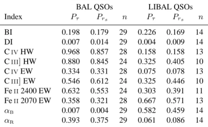
Possible correlations between the polarization degreep0and the various spectral indices were similarly searched for by com-puting the Kendallτ and the Spearman rsstatistics. The result-ing probabilitiesPτandPrsare given in Table 6, for the whole

BAL QSO sample and for LIBAL QSOs only. Note that similar results are obtained when usingp instead of p0. From this table, it appears that the polarization degree is significantly correlated

Fig. 4. The correlation between the polarization degree p0(in%) and

the line profile detachment index DI for all BAL QSOs of our sample. Symbols are as in Fig. 3. The correlation is especially apparent for the QSOs of the LIBAL sample

Table 6. Analysis of correlation between p0and various indices

BAL QSOs LIBAL QSOs

Index Pτ Prs n Pτ Prs n BI 0.198 0.179 29 0.226 0.169 14 DI 0.007 0.014 29 0.004 0.009 14 Civ HW 0.968 0.857 28 0.158 0.158 13 Ciii] HW 0.880 0.845 24 0.325 0.405 10 Civ EW 0.334 0.331 28 0.075 0.078 13 Ciii] EW 0.546 0.612 24 0.325 0.446 10 Feii 2400 EW 0.632 0.553 24 0.303 0.391 11 Feii 2070 EW 0.358 0.321 28 0.667 0.571 13 αB 0.007 0.004 29 0.582 0.459 14 αR 0.393 0.375 29 0.061 0.086 14

with the slope of the continuumαB, and with the line profile

detachment index DI.

The correlation with αB disappears when considering

LIBAL QSOs only, althoughp0andαBstill span a large range of

values. Most probably, this correlation is detected in the whole BAL QSO sample as a consequence of the different distributions of bothαBandp0in the LIBAL and HIBAL QSO sub-samples (Figs. 2 and 3).

On the contrary, the correlation with the detachment index holds for the whole BAL QSO sample as well as for the LIBAL QSO sub-sample. It is illustrated in Fig. 4. In fact, the correlation appears dominated by the behavior of LIBAL QSOs. HIBAL QSOs roughly follow the trend, but their range in DI is not large enough to be sure that they behave similarly4. It is interesting to remark that the observed correlation is stable – and even slightly better – if we assume that the polarization degree increases to-wards shorter wavelengths, i.e. ifp0is redshift-dependent. This

4 _{Note that the apparent difference between the distributions of DI}

for LIBAL and HIBAL QSOs is not significant (PK

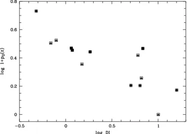
Fig. 5. The correlation between the redshift-corrected polarization

de-gree p0(z) (in%) and the line profile detachment index DI for LIBAL

QSOs only. We assume p0(z) = p0(_1+z3 ), i.e. a λ−1dependence of

p0. Symbols are as in Fig. 3

is as illustrated in Fig. 5 for the LIBAL QSO sub-sample, as-suming a reasonableλ−1_{dependence (e.g. Cohen et al. 1995).} In this case,Pτ = 0.0006 andPrs= 0.0003.

No other correlation ofp0, namely with the balnicity index, or with emission line indices is detected.

5. Discussion and conclusions

New broad-band linear polarization measurements have been obtained for a sample of 42 optically selected QSOs including 29 BAL QSOs (14 LIBAL and 13 HIBAL). The polarization properties of the different sub-classes have been compared, and possible correlations with various spectral indices searched for. The main results of our study are:

– Nearly all highly polarized QSOs of our sample belong to the LIBAL class (provided that BAL QSOs with weaker low-ionization features are included in the class).

– The range of polarization is significantly larger for LIBAL QSOs than for HIBAL and non-BAL QSOs. It extends from 0% to 4.4%, with a peak near 2%.

– There is some indication that HIBAL QSOs as a class may be more polarized than non-BAL QSOs and therefore in-termediate between LIBAL and non-BAL QSOs, but the statistics are not compelling from the sample surveyed thus far.

– We confirm the fact that LIBAL QSOs (including weaker ones) have larger balnicity indices and more reddened con-tinua than HIBAL QSOs.

– The continuum polarization appears correlated with the line

profile detachment index, especially in the LIBAL QSO

sub-sample.

– No correlation is found between polarization and the strength of the low- or the high-ionization absorption fea-tures, nor with the strength or the width of the emission

lines. The apparent correlation between polarization and the slope of the continuum is probably due to the different dis-tribution of these quantities within the HIBAL and LIBAL sub-samples.

The fact that LIBAL QSOs have different polarization prop-erties is an additional piece of evidence that these objects could constitute a different class of radio-quiet QSOs, as suggested by several authors (WMFH, Sprayberry & Foltz 1992, and Boro-son & Meyers 1992), HIBAL QSOs being much more similar to non-BAL QSOs. The higher maximum polarization observed in LIBAL QSOs is probably related to the larger amount of absorb-ing material and/or dust, either via the presence of additional scatterers (dust or electrons), or via an increased attenuation of the direct continuum.

The correlation between the continuum polarization and the detachment index was unexpected, especially since the latter index is a rather subtle characteristic of the line profiles which involves both absorption and emission components. The cor-relation is in the sense that LIBAL QSOs with detachedC iv

profiles are less polarized in the continuum, while those with P Cygni-typeC iv profiles are more polarized. The most

obvi-ous explanation for such a correlation is that the high-ionization line profiles and the continuum polarization both depend on the geometry and/or the orientation of the LIBAL QSOs. This would explain that a range of polarization degrees is in fact observed, the maximum value being characteristic of the class. It is not excluded that HIBAL QSOs behave similarly within a smaller polarization range.

Murray et al. (1995) proposed a BAL flow model which accounts for many of the observed BAL profiles including the detached ones. Instead of being accelerated radially from a cen-tral source, the flow emerges from the accretion disk at some distance from the central source. It is then exposed to the con-tinuum radiation and accelerated, rapidly reaching radial trajec-tories. The wind has naturally a maximum opening angle, and may produce polarization in the continuum via electron scatter-ing. Other recent models are also based on such a “wind-from-disk” paradigm, and may result in roughly similar geometry and kinematics although acceleration mechanisms, photoionization, cloud size and filling factor could significantly differ (de Kool & Begelman 1995, K¨onigl & Kartje 1994, Emmering et al. 1992). Murray et al. (1995) show that for a flow seen nearly along the disk, P Cygni-type profiles with black troughs at low veloc-ities are naturally produced. For the flow seen at grazing angle along the upper edge of the wind, high-velocity detached ab-sorptions are obtained. Since the direct continuum is expected to be more attenuated for lines of sight near the disk, the contin-uum polarization is expected to be higher for orientations which produce P Cygni-type profiles than for orientations which pro-duce detached profiles. This is in good qualitative agreement with the observed correlation. This mechanism has already been proposed by Goodrich (1997) to explain the higher polarization of some PHL5200-like (i.e. P Cygni-type) BAL QSOs. The polarization being uncorrelated with the slope of the contin-uum in the LIBAL QSO sub-sample, this differential

attenua-tion should be dominated by electron scattering in the wind. In fact, the electron scattering models of Brown & McLean (1977) also account for the observed behavior. For the cylindrical sec-tor geometry which roughly characterizes the “wind-from-disk” models, Brown & McLean (1977) found that the observed po-larization is given byp ∝ n0R sin φ cos

2

φ sin2

i, where i is the

inclination of the system (i = 0◦_{for the disk in the plane of} the sky),φ the opening half-angle of the wind, R its maximum

extension, andn0a uniform electron density. With this geome-try, polarization is higher along the equatorial line of sight (i =

90◦_{) than along any other line of sight, again in good agreement} with the observed correlation. In addition to this orientation ef-fect within the LIBAL QSO sub-class, we see that the higher wind opacities (from either density or size) or the larger cover-ing factors (up toφ ∼ 35◦_{) which possibly distinguish LIBAL} QSOs from HIBAL QSOs lead to higher maximum polariza-tions, as observed. While these models are certainly too simple to reproduce quantitatively the observations, the good overall agreement is encouraging.

A problem with the “wind-from-disk” model is that low-ionization features are assumed to be formed near the disk and therefore only observable for nearly equatorial lines of sight (Murray et al. 1995); low-ionization absorption troughs and high-ionization detached profiles are apparently mutually exclu-sive. Since this is not the case observationally, we have to admit that low-ionization features could form at large distance from the core also along inclined views. In this case, low-ionization features could be observed not only at the low-velocity end of the high-ionization troughs, but also at higher velocities. And in-deed, more complex velocity structures are observed in the low-ionization troughs of two LIBAL QSOs with detachedC iv

pro-files, 0335-3339 and 1231+1320 (Voit et al. 1993), giving some support to this hypothesis. Assuming more extended LIBAL regions would also imply that LIBAL and HIBAL QSOs are different objects, in agreement with other studies (e.g. Boroson & Meyers 1992). Possibly, the efficiency of the X-ray shielding could make the difference.

While unexpected a priori, the correlation found between LIBAL QSO line profiles and continuum polarization fits reasonably well the “wind-from-disk” models, without the need of ad-hoc explanations. Clearly, the possibility of more extended LIBAL regions should be investigated theoretically. More detailed polarization differences between objects with detached and with P Cygni-type profiles should be carefully investigated, namely using spectropolarimetry. Also, possible differences between the X-ray properties of LIBAL and HIBAL QSOs would be worthwhile to detect.

Acknowledgements. This research is supported in part by the contract

ARC 94/99-178, and a project funded by SSTC/ Prodex. We would like to thank Jean Surdej for reading the manuscript, and the referee for useful comments.

References

Angonin M.C., Remy M., Surdej J., Vanderriest C., 1990, A&A 233, L5 Arav N., Shlosman I., Weymann R.J., 1997, Mass Ejection from Active

Galactic Nuclei. ASP Conference Series 128, San Francisco Bechtold J., Elvis M., Fiore F., et al., 1994, AJ 108, 374 Becker R.H., Gregg M.D., Hook I., et al., 1997, ApJ 479, L93 Berriman G., Schmidt G.D., West S.C., Stockman H.S., 1990, ApJS

74, 869

Boroson T.A., Meyers K.A., 1992, ApJ 397, 442 Brown J.C., McLean I.S., 1977, A&A 57, 141 Burstein D., Heiles C., 1982, AJ 87, 1165 (BH) Clavel J., 1998, A&A 331, 853

Cohen M.H., Ogle P.M., Tran H.D., et al., 1995, ApJ 448, L77 de Kool M., Begelman M.C., 1995, ApJ 455, 448

di Serego Alighieri S., 1989, In: Grosbøl P.J. et al. (eds.) 1st

ESO/ST-ECF, Data Analysis Workshop, 157

Djorgovski S., Meylan G., 1989, In: Moran J.M. et al. (eds.) Gravita-tional Lenses. Lect. Notes Phys. 330, 173

Emmering R.T., Blandford R.D., Shlosman I., 1992, ApJ 385, 460 Goodrich R.W., Miller J.S., 1995, ApJ 448, L73

Goodrich R.W., 1997, ApJ 474, 606

Hartig G.F., Baldwin J.A., 1986, ApJ 302, 64 (HB)

Hazard C., Morton D.C., Terlevich R., McMahon R., 1984, ApJ 282, 33 Hewett P.C., Foltz C.B., Chaffee F.H., 1995, AJ 109, 1498

Hiltner W.A., 1956, ApJS 2, 389

Hines D.C., Schmidt G.D., 1997, In: Arav N. et al. (eds.) Mass Ejection from Active Galactic Nuclei. ASP Conference Series 128, 59 Hooper E.J., Impey C.D., Foltz C.B., Hewett P.C., 1995, ApJ 445, 62 Hutsem´ekers D., 1993, A&A 280, 435

K¨onigl A., Kartje J.F., 1994, ApJ 434, 446

Korista K.T., Voit G.M., Morris S.L., Weymann R.J., 1993, ApJS 88, 357

Melnick J., Dekker H., D’Odorico S., 1989, EFOSC, ESO operating manual No 4, Version 2, ESO

Meylan G., Djorgovski S., 1989, ApJ 338, L1

Michalitsianos A.G., Oliversen R.J., 1995, ApJ 439, 599 Moore R.L., Stockman H.S., 1981, ApJ 243, 60 Moore R.L., Stockman H.S., 1984, ApJ 279, 465

Murray N., Chiang J., Grossman S.A., Voit G.M., 1995, ApJ 451, 498 Press W.H., Flannery B.P., Teukolsky S.A., Vetterling W.T., 1989,

Nu-merical Recipes, Cambridge University Press Refsdal S., Surdej J., 1994, Rep. Prog. Phys. 56, 117

Reimers D., Bade N., Schartel N., et al., 1995, A&A 296, L49 Schwarz H.E., 1987, In: Polarimetry with EFOSC. ESO Internal

Mem-orandum Dec. 1987

Serkowski K., 1962, In: Kopal Z. (ed.) Advances in Astronomy and Astrophysics. Academic Press 1, 289

Simmons J.F.L., Stewart B.G., 1985, A&A 142, 100 Sprayberry D., Foltz C.B., 1992, ApJ 390, 39 Steidel C.C., Sargent W.L.W. 1992, ApJS 80, 1

Stocke J.T., Morris S.L., Weymann R.J., Foltz C.B., 1992, ApJ 396, 487

Stockman H.S., Moore R.L., Angel J.R.P., 1984, ApJ 279, 485 V´eron M.-P., V´eron P., 1996, A Catalogue of Quasars and Active Nuclei

(7th Edition), ESO Scientific Report 17

Voit G.M., Weymann R.J., Korista K.T., 1993, ApJ 413, 95 Wardle J.F.C., Kronberg P.P., 1974, ApJ 194, 249

Weymann R.J., Morris S.L., Foltz C.B., Hewett P.C., 1991, ApJ 373, 23 (WMFH)