HAL Id: hal-01098701
https://hal.inria.fr/hal-01098701
Submitted on 28 Dec 2014
HAL is a multi-disciplinary open access
archive for the deposit and dissemination of
sci-entific research documents, whether they are
pub-lished or not. The documents may come from
teaching and research institutions in France or
abroad, or from public or private research centers.
L’archive ouverte pluridisciplinaire HAL, est
destinée au dépôt et à la diffusion de documents
scientifiques de niveau recherche, publiés ou non,
émanant des établissements d’enseignement et de
recherche français ou étrangers, des laboratoires
publics ou privés.
Context-based vector fields for multi-object tracking in
application to road traffic
Egor Sattarov, Sergio Alberto Rodriguez Florez, Alexander Gepperth, Roger
Reynaud
To cite this version:
Egor Sattarov, Sergio Alberto Rodriguez Florez, Alexander Gepperth, Roger Reynaud.
Context-based vector fields for multi-object tracking in application to road traffic. IEEE International
Con-ference On Intelligent Transportation Systems (ITSC), Oct 2014, Qingdao, China. pp.1179 - 1185,
�10.1109/ITSC.2014.6957847�. �hal-01098701�
Context-based vector fields for multi-object
tracking in application to road traffic
Egor Sattarov
1,2,3, Sergio A. Rodr´ıguez F.
1,2, Alexander Gepperth
3, Roger Reynaud
1,2 1Universit´e Paris-Sud
,
2CNRS Institut d’ ´
Electronique Fondamentale UMR 8622
3
Ecole Nationale Sup´erieure de Techniques Avanc´ees, France
Abstract—In this contribution, we propose to use road and lane information as contextual cues in order to increase the precision of multi-object object tracking. For tracking, we employ a Monte Carlo implementation of a Probability Hypothesis Density (PHD)-filter, whereas scene context (road and lane information) is taken from annotated street maps. The novel aspect of the presented work is the tightly coupling of context information and the particle filtering process. This is achieved by injecting a priori particles representing locally expected motions, which are in turn determined by the local road and the lane configuration.
This approach is evaluated on objects (tracklets) from the public KITTI benchmark database. Our experimental findings demonstrate a considerable tracking precision increasing when including this kind of a priori knowledge. At the same time, the approach is able to determine objects whose movements differ from the locally expected motion, which is an important feature for safety applications.
Keywords—Multi-tracking, Probability Hypothesis Density Filter, Particle filter, Vector field, Intelligent vehicle, Road context
I. INTRODUCTION
After more than 30 years of contributions on Multiple Target Tracking (MTT), this subject still remains open since, depending on the applications, it addresses complex problems such as management of multiple hypotheses, data association between multiple information sources, and real time constraints. In the context of Intelligent Vehicles (IV), MTT is a key perception process attempting to determine the (e.g. kinematic) state of observed objects. This information is not only important for active safety applications, such as Advanced Driver Assistance Systems (ADAS), but also for scene understanding in autonomous vehicles.
I-A. Related work
Classic MTT approaches are defined by a recursive framework where a set of detected objects is managed by means of temporal filtering such as Kalman or particle filters. Filtering can usually cope with detection errors and simple missed detections. Multiple Hypothesis Tracking (MHT, [14]), and Joint Probability Data Association Filter-ing (JPDAF, [1], [7], are part of well-known mechanisms improving the performance of tracking for complex object-to-track association cases in the presence of missed and false detections.
The PHD filter algorithm is efficient in terms of com-putational resources and propagates the first-order moments of multi-object statistics [10], [17], [12], [19], [18]. PHD is capable to filter clutter, missing observations along with noisy ones using the full Bayesian basis, just like MTT, but with linear complexity depending the number of tracked objects.
Recently, efficient particle implementations of PHD fil-tering have been proposed [18], [10], [12]. These approaches include the estimation of the number of observed tracks. To this end, particle clustering is necessary to identify tracks. However, such a procedure is non-trivial in urban scenarios where objects move in close proximity to each other. In our variant of the particle-based PHD-filter, we avoid the prob-lems of clustering and cardinality estimation by initializing tracks with a fixed number of particles constantly attached to them. The method used by us is not claiming to perform superior multi-object tracking, however, it does facilitate the integration of contextual information, as particles are easy to affect by context information.
Temporal filtering contained in MTT frameworks ex-ploits motion models and observed measurements for max-imizing the probability of the observed motion. Interactive motion models take advantage of multiple expected high-level motion classes, such as lane changes or turns or stops at crossroads in application to IV contexts [6], [3]. Those models use online information about recent vehicle motions to predict their future positions. In our case, no motion model classes have been defined, but low-level primitives have been integrated in the form of expected velocity vector fields. Such vector fields are defined by road and lane context, which is in turn taken from maps using ego-localization information.
I-B. Contribution
Most of the state-of-the-art methods, which exploit con-text information, are strongly correlated to a particular detection method. For instance, road detection approaches [15], [2], [16], [5], are used to provide key information for driving assistance applications or to define regions of interest for object tracking [2], [11]. In contrast, this study is inspired by [9], [8], [13], [11] and aims to use extracted context (road) information to directly improve the quality of multi-object tracking. Our contribution in this article is a computational mechanism for integrating a priori knowledge
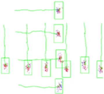
Figure 1: Example of a simulated multi-target tracking scene. Green rectangles are tracks, red circles are detections, dots are particles
derived from contextual road and lane information into a state-of-the-art multi-object tracking system. The benefits of this approach are evaluated in terms of track continuity and track overlapping.
II. PROPOSED METHODS
Our goal is to track vehicles, pedestrians and other possi-ble objects in two-dimensional space (top-view) while taking scene context into account. Two use cases are considered: simulated scenarios on a featureless 2D map plane with hand-crafted velocity vector field as illustrated in Fig. 1, and a 2D East-North map space as shown in Fig. 2 taken from the KITTI-database, from which we obtain object information and GPS coordinates for the extraction of road and lane context via OpenStreetMap.
II-A. PHD-filter-based tracker The PHD filter is represented byNx
dynamically chang-ing tracks xk, k = 1, Nx. Each track x contains Np
particles. Particle ξxk,n,n = 1, N
p contain a set of vectors
{[ci, di, vi]T}, i = 1, D, where D is dimension of the state
space, ci is the center coordinate, di is the detection scale
andviis the speed. A weightωxk,n,n = 1, N
pis assigned to
each particleξxk,n,n = 1, N
p. The parameters of the PHD
filter are: death probability Pd, birth probability Pb, false
negative probability Pf n and a vector of resampling and
association parameters σi, i = 1, D. The tracking process
is composed of the following stages: prediction, association, observation, resampling, merging and correction.
1) Prediction : Tracks and theirs particles are propagated according to the motion model:
ci,t|t−1=ci,t−1+ vi,t−1 (1)
di,t|t−1= di,t−1, i = 1, D (2)
vi,t|t−1= vi,t−1 (3)
wheret is a timestamp and t − 1 is a previous timestamp.
2) Association : Input observationszj, wherej = 1, Nz
andNz
is a number of observations, are assigned to existing tracks xk, k = 1, Nx. Tracks assigned to observations
increase their associated probability by Pd:
Pk,t= max(Pk,t−1+ Pd, 1), k = 1, Nx (4)
Non-associated tracks update their probability by:
Pk,t= max(Pk,t−1− Pd, 0) (5)
Observations which are not associated create new tracks with a probability:
Pk,t= Pb (6)
In case a new track is created, the weights of its particles are:
ωxk,n= Pk,t/N
p
, n = 1, Np (7)
In detail, we proceed as follows:
– For all pairs {zj, xk}, j = 1, Nz; k = 1, Nx the
distanceG(xk,t, zj,t) is calculated, where the distance
function is a product of Gaussians:
G(xk,t, zj,t) = N (cxk,i− czj,i|0, Kcσi) (8)
×N (dxk,i− dzj,i|0, Kdσi)
×N (vxk,i− vzj,i|0, Kvσi)
whereKc, Kd, Kv are coefficients in the range(0, 1],
chosen empirically.
– Calculate an association thresholdθa
, as a distance: θa = G(xk,t, ˆxk,t) (9) where: cxˆk,i= cxk,i+ Kcσi (10) dxˆk,i= dxk,i+ Kdσi (11) vxˆk,i= vxk,i+ Kvσi (12)
– Find the nearest pair
(x, z) = arg max
xk∈X,zj∈Z
G(xk, zj) (13)
Associate these x and z, remove x from list of pairs to associate and repeat this step if:
G(x, z) > θa
(14) – Finally, a list of associated pairs{zj, xk}, a list of
non-associated detections{zj} and a list of non-associated
tracks{xk} are obtained.
3) Observation : For each new observation zj,t, j =
1, Nz
, and for each particle ξxk, xk ∈ X a distance
is calculated: G(ξxk, zj,t). The distances are normalized
relative to observations: ωxk,n= X j G(ξxk, zj) P lG(ξxl, zj) + ωxk,n× Pf n (15)
The last term represents the ”old” particle weights in order to stabilize fluctuations.
4) Resampling : Trackxk is deleted if
Pk < θd (16)
Whereθd
is an imposed parameter. Otherwise, its particles are resampled using random fluctuations:
ci,t= ci,t|t−1+ ζc(0, ˆKcσi) (17)
di,t= di,t|t−1+ ζd(0, ˆKdσi) (18)
vi,t= vi,t|t−1+ ζv(0, ˆKvσi) (19)
Here ζc, ζd, ζv are different white noises, and ˆKc, ˆKd, ˆKv
are coefficients, chosen empirically.
The special multiplier Kˆ increases parameters ˆ
Kc, ˆKd, ˆKv if track’s probability is lower than one
(this is done in order to make particles more dispersed when a track is ”lost”, making it easier to ”pick up” the track later).
5) Merging: If two tracksxk1 andxk2 have a distance:
G(xk1, xk2) > θm (20)
they are supposed to belong to a single object, and the newer track is deleted. Hereθm
is a predefined merging threshold. 6) Correction: New track centers are calculated as the weighted mean of particles associated to that track:
xk,t= 1 Np X n=1,Np ξxk,n,t (21)
The output of the algorithm is represented as a set of tracks. II-B. Vector field implementation
The context information to implement in the tracking system is represented as a vector field, that is, a field of probable directions for each map location. IfΠ is the state space of tracking having dimensionD, and a subspace T ⊂ Π is a space where vector fields are defined, then one point τ ∈ T contains a set of Nτ
vectors V in it. One vector v ∈ V has components vi,i = 1, D.
1) Orientation and norm influence: A track’s coordinates ci, i = 1, D indicate a point of the tracking space π ∈ Π.
At the resampling and association stages, when random fluctuations at point π ∈ T are needed, the vector field is applied. The N × (1 − CM F) first particles are resampled
as in eqns.(17,18,19), and other particles are resampled according to vectors, defined in π in eqns.(22,23,24). Here CM F is a coefficient of ”model force”. Particle resampling
is performed as follows:
ci,t= ci,t|t−1+ ζc (22)
di,t= di,t|t−1+ ζd (23)
vi,t = vπj,i+ ζv (24)
wherevπj is a vector defined at the pointπ, with components
vπj,i, i = 1, D . All N × CM F field-defined particles are
divided between vectorsvπj,j = 1, N
πuniformly. HereNπ
is a number of vectors defined inπ.
Figure 3: An example of a simulated scenario. The color of particles shows their weight and thus their current impact. The red particles have more weight than blue ones. Green rectangles indicate current tracks.
2) Direction-only influence: Another potential way to incorporate context consists in letting only the orientation of the vector field influence tracking. In this case, one can calculate new vector components as follows:
ˆ vπj,i= vπj,i× vt|t−1 vπj (25) Here vt|t−1
is the norm of the track’s speed and vπj
is the norm of the vector field’s speed at πj. So, we fuse the
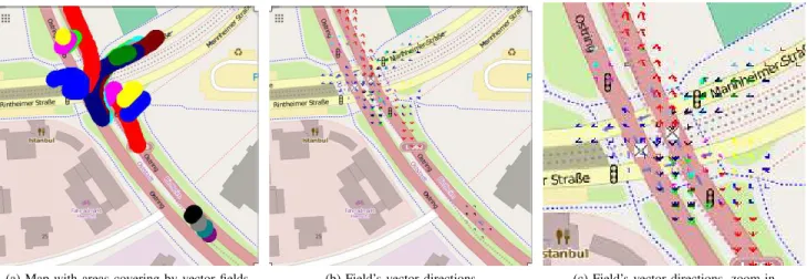
field’s orientation with the norm of the current track’s speed. A visual representation of the vector field for the road map is illustrated in Fig. 2
Especially the second point is important as it eliminates the need to use vector fields containing all possible speeds (vector lengths).
II-C. Vector field compatibility measurement
When the field of possible directions is imposed, it is clear that a moving object may not at all follow these directions. In such a case, it may be assumed that the object has atypical behavior and is therefore potentially dangerous. The detection of such objects is possible with the proposed framework. If the motion of a tracked object satisfies the condition (26) for at least one j, it can be classified as typical. The condition considers motion as being ”typical” if field-sampled particles are closer to new detections than the mean of all particles. Fig. 3 shows a visual distribution of particles’ weights. P n∈ ˆNπjωxk,n P n∈ ˆNpωxk,n × N p CM F/Nπj > 1 (26)
Here, ˆN and ˆNπj are the sets of indexes for all particles
of object and particles, resampled according to vector j of pointπ respectively.
(a) Map with areas covering by vector fields (b) Field’s vector directions (c) Field’s vector directions, zoom-in
Figure 2: Visual representation of vector fields on a OpenStreetMap (OSM) map
II-D. Evaluation method
Two major evaluation methods are used to quantify the accuracy of our approach: an overlap measure and a continuity measure. The first method measures the accuracy of a track’s position with respect to associated real object position. The ”continuity” measure computes the quality object-to-track associations. Track overlap is calculated as the mean of all association overlaps (i.e. overlap between track and real object):
Overlap= 1 Nassoc X (k,i) max(S(xk∩ yi) S(xk) ,S(xk∩ yi) S(yi) ) (27)
whereNassoc is a number of associations in XZassoc and
S(·) is an area occupied by detection. The overlap value is always ∈ [0, 1], where 1 represents the ideal case of full overlap.
The ”continuity” measure is calculated according to the formula: Continuity= 1 NY X yi∈Y max k 1 Nyi X t δk,i(t) (28)
whereNY is a number of ground-truth objects, Nyi is the
number of appearances of the object yi during the whole
tracking scenario, δk,i(t) = 1 if (k, i) ∈ XZassoc(t) and
δk,i(t) = 0 otherwise. The continuity measure thus describes
the mean of the longest associations. It varies in(0, 1], where 1 is the ideal case of constant associations.
III. EXPERIMENTS
The approach was tested on simulated data and on the public KITTI benchmark dataset[4] using annotated tracklets as ground-truth. The common schema to evaluate results requires four sets of data:
1. The set of labeled rectangles representing tracks constructed by our algorithms:X.
2. The set of labeled rectangles representing real objects Y , or ground-truth.
3. The set of labeled rectangles representing noisy objects Z. It is obtained from ground-truth by artificially introducing missed (false negative) de-tections, and by corrupting retained detections by noise. Noise is modeled as an additional Gaussian fluctuation applied to positions and sizes (ci, di),
i = 1, D of all ground-truth objects. Each noisy detectionz ∈ Z has a ground-truth pair y ∈ Y . 4. The set of pairs of labels representing associations
between noisy detections and tracksXZassoc
As the particle implementation of PHD-filtering contains a pseudo-random process, small variations can occur over trials. To precisely calculate the evaluation measures, the results were calculated as the mean and the variation of both measures across 15 trials.
III-A. Simulation
The first simulation scenario represents a scene of size 1000 × 1000 pixels and of 110 frames, with 10 objects moving simultaneously: four from left to right, six from up to down as shown in Fig. 4a. This scenario is chosen since it contains many pairwise intersections, in order to observe the algorithm’s capability to resolve collisions. All of objects have sizes of30 × 60 pixels.
Noise parameters were set as follows:
1. σd = 10 - the variance of white noise applied to
particle dimensions
2. σc = 30 - the variance of white noise applied to
particle centers
3. False negative ratePf n= 0.1
4. False positive ratePf p= 0.2
(a) (b)
(c)
Figure 4: Visual representation of the vector field (c) and simulated scenarios (a,b). Green rectangles and traces are tracks and their previous positions
1. Pb= 0.7
2. Pd= 0.1
3. Pf n = 0.1
The vector field map was created manually and covers all of the scene uniformly with two directions present: ”right” and ”down” as shown at Fig. 4c.
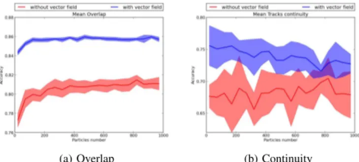
Estimations of overlap and continuity are shown at Fig. 5. A larger improvement of evaluation measures is observed for the overlap, i.e., position estimation, and a lower one for time continuity. However both measures are consistently improved by the introduction of the vector field. Errors of associations can happen mostly in case of intersections. If two tracks meet at one point, they lose parts of their particle information which can help to resolve the collision because vector fields are identical and come from the same point position. But, on the other hand, if two differently oriented tracks meet in one point, the vector field at this point helps them to go through it faster. These two reasons balance themselves and so the impact of the vector field is low.
The overlap errors arise from imprecise positions of associations. When the position noise is Gaussian, the trajec-tories of tracks try to oscillate. When applying vector fields, this stabilizes positions and thus brings them closer to their mean, i.e. to real state.
For the same simulated scenario, vector field compati-bility measures were calculated according to Sec. II-C. We
(a) Overlap (b) Continuity
Figure 5: Accuracy for simulated data when only vector directions are used, plotted as a function of total particle number. Solid lines are mean values, semi-transparent bor-ders represent their variances
Figure 6: Direction compatibility measurements for simu-lated data. The values are calcusimu-lated according to eqn. (26). For values bigger than 1.0, we assume movement along the field, and against the field otherwise.
measured their mean and standard deviation, both for ”com-patible” and ”incom”com-patible” tracks, with the expectation that the compatibility measure allows to distinguish those cases. The compatible tracks were evaluated in the scenario described above, the incompatible ones in a scenario with an inverted vector field but which was otherwise identical. The results are shown in Fig. 6. The difference in mean values is evident, but noise deviations are considerable.
The second simulation scenario represents a scene of size 1000 × 1000 pixels and of 200 frames, with 8 objects si-multaneously: four compatible and four incompatible as it is shown at Fig. 4b. All of objects have sizes of15×15 pixels. Noise parameters were set as follows: σd = 10, σc = 20,
Pf n = 0.2, Pf p = 0.125. PHD imposed parameters are:
Pb = 0.7, Pd = 0.1, Pf n = 0.5. This scenario is used to
test auto-determined model force mechanism. III-B. Real data
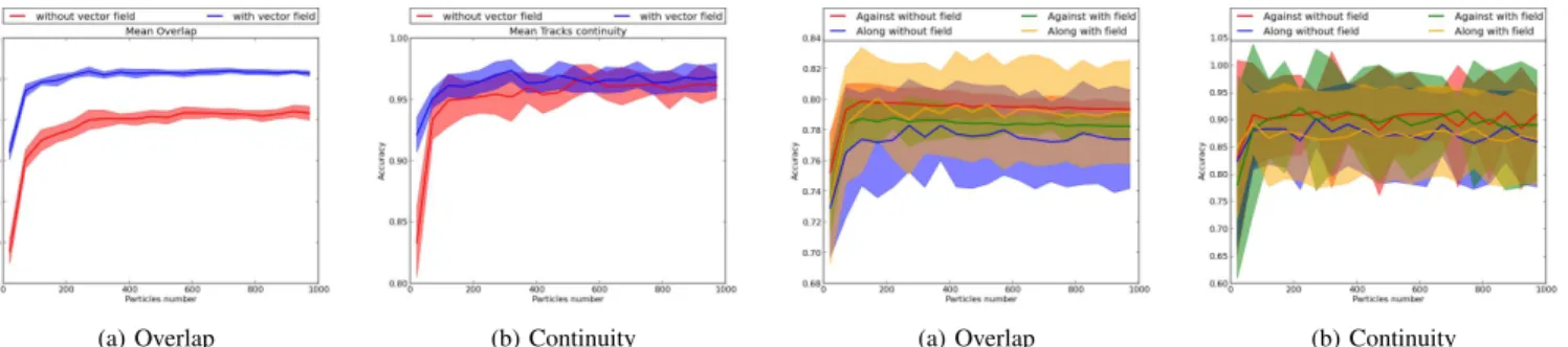
The tracking space is a 2D East-North plane limited of size 165 × 167 meters shown in Fig. 2. The duration of tracking is 12 seconds with a frequency of 8.9 f ps. A number of 19 targets takes part in this urban traffic scenario. Since objects like cars, buses, pedestrians and cyclists are present without class distinction, detections of pedestrians can be mixed with detections of cars and other objects.
(a) Overlap (b) Continuity
Figure 7: Accuracy for real data for both vector directions and norms used in dependency of used particles number
(a) Overlap (b) Continuity
Figure 8: Accuracy for real data for only vector directions used in dependency of used particles number
Noise parameters were set to:σd = 0, σc = 0.5 meters,
Pf n = 0.1, Pf p = 0. PHD imposed parameters are: Pb =
0.7, Pd= 0.1, Pf n= 0.1.
The vector field map was created manually based on OpenStreetMap and KITTI Velodyne and GPS-data and covers all tracklets’ possible occupation areas with directions collateral to expected target motions in those areas. The map of directions is displayed in Figs. 2b,2c
Estimations of overlap and continuity in cases of full information are shown at Figs. 7,8. As in case of simulated data, the overlap shows a greater performance difference as a consequence of the vector field. The variance of performance is smaller because of less noise occurring in the real scenario.
From the comparison of the two cases: direction+norm vs direction only, and from the comparison of margins between baseline and vector field-affected performance, it is possible to draw the conclusion that in real road traffic the value of speed is a helpful information, but that one can still obtain significant gains in tracking quality when using only directions.
III-C. Auto-determined model force
The second simulated scenario mentioned in Sec. III-A was created to compare the impact on tracking precision
(a) Overlap (b) Continuity
Figure 9: Comparison of accuracy for tracks moving along and against vector fields without and with them using fixed model force coefficient
(a) Overlap (b) Continuity
Figure 10: Comparison of accuracy for tracks moving along and against vector fields without and with them using a variable model force coefficient
in the case of movements along vector fields to the case of movements against it. As expected, the results obtained during this experiment show a decreased tracking perfor-mance when tracks are incompatible with the context fields. In Fig. 9, four lines are shown where blue and red are the respective baselines for compatible and incompatible tracks without the influence of vector fields. Yellow and green curves represent compatible and incompatible tracks assisted by context with a fixed model force coefficient, CM F = 0.05. As illustrated, the overlap observed for
incom-patible tracks is the almost the same as the improvement for compatible ones. Track continuity seems not be influenced in both cases.
Hereafter, we addressed the question of how to keep the advantages of contextual information while reducing the undesirable effects on incompatible tracks. To this end, a dynamic estimation of the model force coefficient, CM F,
is proposed. If the track is considered as compatible with respect to the vector field, see eqn. (26), CM F is increased
by 0.01 or decreased otherwise. For all tracks,CM F varies
from 0.01 to 0.5. The results are shown in Fig. 10
The overlap improvement for compatible tracks clearly outweighs the slight performance decrease observed for incompatible ones. However, track continuity decreases
par-ticularly for compatible tracks. This result can be explained in ambiguous tracking situations (e.g. two tracks intersect-ing) where contextual information can induce object-to-track association errors. Simulated scenarios contain objects intersecting at the same location with different speed direc-tions. This use case is however not encountered under real conditions.
IV. DISCUSSION
We presented a principled method to introduce prior knowledge into tracking, in this case information about expected object speeds obtained from scene context. We showed, both in a simulated and a real scenario from the KITTI database, that the quality of tracking (measured by standard measures) is significantly improved, leading to a more robust trajectory and motion estimation by a tracking algorithm. Although different tracking algorithms will implement this differently, the proposed vector field approach can be transferred to all particle-based tracking models and thus has a rather wide range of applicability.
Please note that, in this article, we have not addressed the subject of object detection: object information, or ground-truth, is available in both the simulated and the real scenario that we consider, and we corrupt it artificially by noise in order to show the benefits of our approach. Particularly when detections are obtained, as it is envisioned, from a real object detection system, our approach will be beneficial because the motion priors may conceivably lead to a better position estimation than it would be possible from noisy detections alone.
The Gaussian noise applied to simulate the detection jitter is not very realistic, and results may be slightly worse for a less convenient noise model. However it is simple to implement, and gives a good guess of performance under noise.
V. CONCLUSION
In this paper, we presented a proof-of-concept of a novel method for multiple target tracking for Intelligent Vehicles. This method uses road information in order to provide con-textual cues which lead to an increased precision in multi-object tracking, suing a PHD filter approach in it’s particle implementation. The public KITTI benchmark database was used to verify the impact on tracking precision, providing that such kind of a priori knowledge is considerably helpful when there is no single a priori direction but a distribution over them. The automatic detection of objects that violate the imposed priors was studied with favorable results, promising applicability in safety applications. Several points are still open, in particular how to correctly encode vector fields (with or without speed component). A subset of Gaussian-distributed particles with modified speed vectors, as used in this article, is a possibility, but other distributions, or a more complex particle state including potential high-level behaviors, are conceivable as well. Immediate future work will include a more representative testing using a marge set
of urban traffic scenarios, provide more findings regarding the robustness of the proposed methodology.
REFERENCES
[1] Habtemariam B., Tharmarasa R., Thayaparan T., and Mallick M. A multiple-detection joint probabilistic data association filter. 7:461 – 471, 2013.
[2] Roland Chapuis, Romuald Aufrere, and Fr´ed´eric Chausse. Accurate road following and reconstruction by computer vision. volume 3, pages 261 – 270. IEEE, Transactions on Intelligent Transportation Systems, 2002.
[3] Yang Cheng and Tarunraj Singh. Efficient particle filtering for road-constrained target tracking. 43, 2007.
[4] Jannik Fritsch, Tobias Kuehnl, and Andreas Geiger. A new per-formance measure and evaluation benchmark for road detection algorithms. In IEEE 16th International Conference on Intelligent
Transportation Systems (ITSC), pages 1693 – 1700, 2013. [5] Xiao Hu, Sergio A. Rodr´ıguez F., and Alexander Gepperth. A
multi-modal system for road detection and segmentation. pages 1365 – 1370. IEEE, Intelligent Vehicles Symposium Proceedings, 2014. [6] Zhentao Hu, Yong Jin, Jie Li, and Xianxing Liu. Maneuvering
target tracking algorithm based on multiple model rao-blackwellised particle filter. Journal of Information and Computational Science, 8, 2012.
[7] Lim Jaechan. The joint probabilistic data association filter (jpdaf) for multi-target tracking. Technical report, Stony Brook University, 2006.
[8] Julian F. P. Kooij, Nicolas Schneider, and Dariu M. Gavrila. Analysis of pedestrian dynamics from a vehicle perspective. pages 1445 – 1450. IEEE, Intelligent Vehicles Symposium Proceedings, 2014. [9] Emilio Maggio and Andrea Cavallaro. Learning scene context for
multiple object tracking. volume 18, pages 1873 – 1884. Transactions on Image Processing, IEEE, 2009.
[10] Emilio Maggio, Elisa Piccardo, Carlo Regazzoni, and Andrea Caval-laro. Particle phd filtering for multi-target visual tracking. volume 1, pages I–1101 – I–1104. IEEE International Conference on Acoustics, Speech and Signal Processing, 2007.
[11] Umut Orguner, Thomas Sch¨on, and Fredrik Gustafsson. Improved target tracking with road network information. pages 1 – 11, 2009. [12] Marek Schikora, Amadou Gning, and Lyudmila Mihaylova. Box-particle phd filter for multi-target tracking. pages 106 – 113. 15th International Conference on Information Fusion (FUSION), 2012. [13] Naoki Shibata, Seiji Sugiyama, and Takahiro Wada. Collision
avoidance control with steering using velocity potential field. pages 438 – 443. IEEE, Intelligent Vehicles Symposium Proceedings, 2014. [14] Blackman S.S. Multiple hypothesis tracking for muliple target
tracking. 19:5 – 18, 2004.
[15] Sarah Strygulecy, Dennis Muller, Mirko Meuter, Christian Nunn, Sharmila (Lali) Ghosh, and Christian Wohlery. Road boundary detection and tracking using monochrome camera images. pages 864 – 870. IEEE, 16th International Conference on Information Fusion (FUSION), 2013.
[16] M. Ulmke and W. Koch. Road map extraction using gmti tracking. pages 1 – 7. IEEE, 9th International Conference on Information Fusion (FUSION), 2006.
[17] Ba-Ngu Vo and Wing-Kin Ma. The gaussian mixture probability hypothesis density filter. volume 54, pages 4091 – 4104. Transactions on Signal Processing, IEEE, 2006.
[18] Ba-Ngu Vo, Sumeetpal Singh, and Arnaud Doucet. Sequential monte carlo implementation of the phd filter for multi-target tracking. 2:792 – 799, 2003.
[19] Yunmei Zheng, Zhiguo Shi, Rongxing Lu, Shaohua Hong, and Xuemin (Sherman) Shen. An efficient data-driven particle phd filter for multi-target tracking. 9:2318 – 2326, 2013.