Climate Dynamics (1999) 15 : 569}581 ( Springer-Verlag 1999
J. Guiot ' J. J. Boreux ' P. Braconnot ' F. Torre
PMIP participants
Data-model comparison using fuzzy logic in paleoclimatology
Received: 27 May 1998 / Accepted: 8 January 1999
Abstract Until now, most paleoclimate model-data
comparisons have been limited to simple statistical
evaluation and simple map comparisons. We have
ap-plied a new method, based on fuzzy logic, to the
com-parison of 17 model simulations of the mid-Holocene
(6 ka BP) climate with reconstruction of three
bio-climatic parameters (mean temperature of the coldest
month, MTCO, growing degree-days above 5 3C,
GDD5, precipitation minus evapotranspiration, P!E)
from pollen and lake-status data over Europe. With
this method, no assumption is made about the
distribu-tion of the signal and on its error, and both the error
bars related to data and to model simulations are taken
into account. Data are taken at the drilling sites (not
using a gridded interpolation of proxy data) and
a varying domain size of comparison enables us to
make the best common resolution between observed
and simulated maps. For each parameter and each
model, we compute a Hagaman distance which gives an
objective measure of the goodness of "t between model
and data. The results show that there is no systematic
order for the three climatic parameters between
mod-els. None of the models is able to satisfactorily
repro-duce the three pollen-derived data. There is larger
dispersion in the results for MTCO and P!E than
for GDD5. There is also no systematic relationship
between model resolution and the Hagaman distance,
except for P!E. The more local character of P!E
J. Guiot (|) ) F. Torre
IMEP, CNRS UPRES A6116, FaculteH de St-JeHro(me, Case 451, 13397 Marseille Cedex 20, France
E-mail: Joel.Guiot@lbhp.u-3mrs.fr J. J. Boreux
Fondation Universitaire Luxembourgeoise, Avenue de Longwy, 185, 6700 Arlon, Belgique
P. Braconnot
LSCE, CEA-DSM, Orme des merisiers, CE-Saclay, 91191 Gif sur Yvette Cedex, France
has little chance to be reproduced by a low resolution
model, which can explain the inverse relationship
be-tween model resolution and Hagaman distance. The
results also reveal that most of the models are better at
predicting 6 ka climate than the modern climate.
1 Introduction
One of the aims of the Paleoclimate Modeling
Inter-comparison Project (PMIP) (Joussaume and Taylor
1995) is to assess the ability of atmospheric general
circulation models (AGCMs) to represent a climate
di!erent from the present day. Most of the models
involved in PMIP are used in simulation of
anthropo-genic climate change (Kattenberg et al. 1995), and we
therefore need to know if those models are able to
successfully represent a climate di!erent from the
pres-ent one. This can be achieved using paleoclimate data.
The 6000 yr BP climate has been chosen as a key period
for PMIP because it is a simple experiment from a
modelling point of view, and it is data rich. Indeed, for
this period, several paleoclimatic data sets are now
available for di!erent regions of the globe (Wright et al.
1994), and considerable e!ort has been made to
syn-thesise available data and building comprehensive data
sets that can be used for model-data comparisons
(Wright et al. 1994; Prentice et al. 1996; Cheddadi et al.
1997; Harrison et al. 1996; Jolly et al. 1998).
Up to now, most model-data comparisons using
paleoclimate data (Liao et al. 1994; Prentice et al. 1998;
Dong and Valdes 1995; Texier et al. 1997; Masson et al.
1999) have been limited to simple maps or data
com-parison in a few regions, and only simple statistics have
been used. The biome model of Prentice et al. (1992)
has also proved e$cient in translating model
out-puts into biomes that can be directly compared with
pollen data reconstuctions of past vegetation (Texier
et al. 1997; Harrison et al. 1998). In these cases, kappa
statistics (Monserud and Leemans 1992) are used
to measure how di!erent the reconstructed vegetation
is from the present-day one. As long as only one model
is considered and model-data di!erences are large,
ob-vious mismatches between observations and model
output can help identify weaknesses in the model's
ability to reproduce natural events. However when
several models are considered or when model-data
di!erences are small, there arises the need for
synthesis-ing subtle di!erences at many spatial points, which
can only be achieved with an objective measure of
the goodness of "t between model and reality. The
present study extends the work of Masson et al.
(1999) in comparing PMIP model results over
Europe with bioclimatic variables (temperature of
the coldest month, growing degree days and
precipita-tion minus evaporaprecipita-tion) reconstructed from pollen
data (Cheddadi et al. 1997), by introducing a
new objective measure of the goodness of "t between
model and data and using it to classify the model
performances.
Preisendorfer and Barnett (1983), have pointed
out that a measure of the goodness of "t between
model and reality should be adjustable to allow both
a local and global intercomparison, and that it is also
needed to assign a measure of the signi"cance to that
measure of the "t. Frankignoul et al. (1989) and
Braconnot and Frankignoul (1993) demonstrated that
it was also very important to include all sources of
uncertainties arising either from measurement errors,
data sampling, small- scale variability of model forcing
in the comparison. There is indeed no need to discuss
di!erences in regions where neither data nor the model
outputs are reliable. Evaluation of model performances
are intrinsically linked to a speci"c model or problem,
which explains why there is not a universal method for
model testing. Instead, di!erent approaches using
either parametric or non parametric statistics have
been developed in atmospheric and oceanic sciences
(e.g. Mielke et al. 1981; Preisendorfer and Barnett
1983; Willmott et al. 1985; Zwiers and Storch 1989;
Frankignoul et al. 1989; Braconnot and Frankignoul
1993, 1994). These methods deal with data generated
at a large number of grid cells which are spatially
autocorrelated, and small samples. This is why prior
to model-data comparison, data compression is usually
performed using principal component analysis or its
derivatives, such as common empirical orthogonal
func-tion (EOF) analyses (Duche(ne and Frankignoul 1991;
Braconnot and Frankignoul 1993, 1994; Frankignoul
et al. 1995). In all these above mentioned applications,
model outputs and observations were interpolated
on a common grid. This procedure is not a problem
for present day climate when observations are quite
numerous, and when it is possible to have an
esti-mate of the uncertainties in poorly covered data, but it
may be one for the sparser networks of paleoclimatic
data.
For paleoclimate studies, even with the most
com-plete data set available, the data coverage is poor and
not regularly spaced, and is characterised by di!erent
spatial scales of variability from local to synoptic. The
data used for comparison in this study (Cheddadi et al.
1997) have been interpolated by the authors on a
regu-lar grid. Because this interpolation could be in#uenced
by remote points in regions of inadequate sampling,
it is di$cult to de"ne the reliability of the gridded
re-construction. We have therefore decided to de"ne a
method that can work without interpolation on a
com-mon grid. Pollen data are taken at the location of
drilling, and each model is tested against the data on its
own grid.
Ideally, we would also like the goodness-of-"t
measure to re#ect (i.e. to be larger than) those
situ-ations when a model correctly simulates a particular
structure in the data but shifted in location, as opposed
to those situations when the structure is not simulated
at all (e.g. getting an enhanced monsoon, but not
exactly the right place versus not getting an enhanced
monsoon at all). Point-by-point similarities in the
former case (structure present, but geographically
shifted) are likely to be disappointingly small. Finally,
the method must also be able to take into account
the uncertainties of both the pollen-derived variables
and model outputs. In our case, the main source of
data uncertainties comes from the possibly large
tolerance of plants to various climates. For the
atmo-spheric models, the uncertainties arise from initial
conditions, internal variability and surface boundary
conditions (which includes incomplete experimental
design that "xes SSTs and leaves 6 ka vegetation
distribution at modern levels). The errors of the initial
conditions can be neglected, since each model
simula-tion is 15 y long and the atmosphere loses the memory
of the initial conditions in one year. The surface
boundary conditions introduce systematic biases but
they cannot be considered here and will be part of the
mismatch between model and data. The only
uncer-tainty that can be explicitly considered is the internal
variability, which can be estimated from the 15-y
ex-periments.
In summary, we will develop a distance-type
good-ness-of-"t measure able to take into account the
di!er-ence of resolution between AGCM and data maps, the
possible irregularity in the network of data, and the
uncertainties in the data and AGCM simulations.
Moreover, this measure must not be limited to
point-to-point comparisons, but must also allow area-to-area
comparisons so that a slight shift in latitude or/and in
longitude will not be penalised too strongly in the
distance values.
We have adopted a method based on fuzzy logic
(Zimmermann 1985) which is well adapted to our
prob-lem. The method is described in Sect. 2 and applied to
the comparison of PMIP simulations with pollen data
over Europe in Sect. 3.
Fig. 1 Four fuzzy subsets to describe air temperature (3C). An element x in the universe X, here the real interval 5 3C to 35 3C, belongs to each fuzzy subset with a degree of membership between zero and one
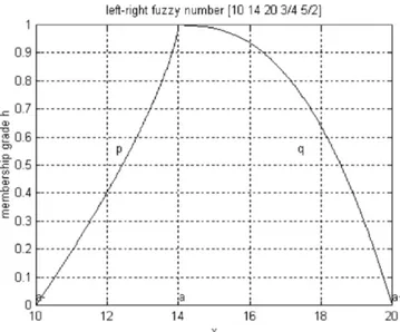
Fig. 2 An example of left-right fuzzy number where a"10, a"14,
a`"20, p"3/4 and q"5/2
2 Method based on fuzzy logic
Fuzzy logic di!ers from conventional logic in that it aims to provide techniques for approximate rather than precise reasoning. Unlike classical statistics which is based on frequency distributions of random populations, fuzzy logic deals with describing the characteristics of properties by associating intervals of continuous variables with semantic labels. The power of this approach comes from the fact that these semantic intervals can or even should overlap.
As an example, consider the parameter &&air temperature''. This parameter can be broken down into four subsets: &&cold'', &&cool'', &&warm'', &&hot''. The domain from the smallest to the largest allow-able value is called the universe of discourse and is denoted X. In Fig. 1, we assume that X is the real interval from 5 to 35 3C. Assume that the actual air temperature, say x0, is 25 3C. We can see that x0 is included in both the &&warm'' and the &&hot'' subset. The di!erence lies in the degree of membership. This particular value of air temper-ature x0 "25 3C belongs to the subset &&warm'' with a degree of membership of 0.8 while it is only 0.2 for the subset &&hot''. Moreover,
x0 does not belong either to the subset &&cold'' or to the subset &&cool''.
So, the degree of membership of x0 is equal to zero for both.Subsets like &&cold'', &&cool'', &&warm'' and &&hot'' are called fuzzy
subsets of X because each element x of X may belong to any subset with a degree of membership varying between zero and one. In others words, fuzzy logic is a graduated logic based on the idea of membership function from the universe of discourse X to the real interval [0,1]. Each element x of the universe of the discourse X is associated with a real number between zero and one giving its degree of membership ful"lment to the subset being considered.
As a contrast, in binary logic, any element x of X cannot be at the same time warm and hot and the corresponding degree of member-ship is one or zero. In fuzzy logic, an ordinary set is called a &&crisp'' set. To distinguish between fuzzy and crisp concepts, fuzzy subsets
will be always denoted with a tilde (I ).
Assume AI is a fuzzy subset of X with membership function kA(x)
(Fig. 1 illustrates particular triangular cases). It must be emphasised that the universe of discourse X is a crisp set, often the set of real numbers. The open interval that ranges from the smallest to the largest value of the universe of the discourse is called the &&support''
of AI . The closed interval consisting of all elements with a degree of
membership equal to 1 is called the &&core'' of the fuzzy subset AI .
Some fuzzy subsets have the empty set as a core. If the core contains only one element this element is called the &&pivot'' of the fuzzy
subset. Thus any fuzzy subset AI is completely de"ned by its
member-ship functionkA(x) which involves both support and core.
2.1 Fuzzy numbers
Fuzzy numbers are special fuzzy subsets. AI is a fuzzy number if and
only if: (1) the universe of discourse X is the set of real numbers; (2) at least one element x of the support has its degree of membership equal to 1 (normal assumption, i.e. the core exists); and (3) the membership function does not have local extrema (i.e. it is assumed to be convex).
Two latter properties limit the shape that a fuzzy number can take: it is always decreasing to the left of the core and non-increasing to the right of the core. So, a real number can be seen as a fuzzy number whose support comprises only one element which has a degree of membership exactly equal to 1.
2.2 The left-right fuzzy numbers or LRFN
The simplest type of fuzzy number has a triangular or trapezoidal membership function (Fig. 1). A more general class of fuzzy numbers is the left-right fuzzy numbers with curvilinear membership func-tions (Dubois and Prade 1980).
Assume a fuzzy number AI with support ]a~, a`[ (this kind of
bracket indicates an open interval), pivot MaN and membership
functionkA(x). This latter can be broken down into a left function
denoted ¸A(x) and a right function denoted RA(x) which have a simple analytic form:
kA(x)" i g j g k ¸A(x)"1!((a!x)/(a!a~))pA x3 ]a~,a]
RA(x)"1!((x!a)/(a`!a))qA x3 [a, a`[
0 otherwise
(1)
where both exponents pA and qA are positive real numbers, that determine how sharply the membership function curves are (Fig. 2). The left bracket ] indicates an interval open at left and the right bracket [ indicates an interval open at right. The subscript &&A'' in
Fig. 3 The Hagaman distance between two triangular fuzzy
num-bers Fig. 4 The minimum distance between triangular fuzzy number
(!5, 0, 3, 1, 1) and triangular fuzzy number of pivot 2 is reached for left spread "9 and right spread 0, giving the TFN equal to (!7, 2, 2, 1, 1): representation of these numbers (in fact the right spread cannot be negative)
Eq. (1) and anywhere in the current text refers to the fuzzy number AI .
Thus relationship Eq. (1) de"nes left-right fuzzy numbers (LRFN). The left-right fuzzy number concept allows us to represent not only the data but also the uncertainty in the data. A large value for both exponents gives a &&fat'' fuzzy number because each x of its support is thought highly possible (almost total uncertainty). In the opposite case, values less than one produce a &&slim'' fuzzy number because only the elements x near the pivot are thought highly possible (almost total certainty). The linear case deals with p"q"1
(triangular fuzzy number or TFN). Therefore, any LRFN AI is
completely de"ned with "ve real numbers: AI ,Ma~,a,a`,pA,qAN.
2.3 Distance between two fuzzy numbers (Hagaman's distance)
A degree of membership of a fuzzy number, AI , is denoted by h and is
de"ned, for all real x, bykA(x). Conversely, for each AI, given a level
h in [0,1], the corresponding abscissa is x"a~(h) for the left side
and x"a`(h) for the right side. So, we de"ne the squared distance between two fuzzy numbers (Fig. 3) as follows (Bardossy et al. 1990, 1993):
D2(AI, BI)"1:
0M(a~(h)!b~(h))2#(a`(h)!b`(h))2Nhdh
(2) In short, relationship (2) is a weighted average squared distance
between AI and BI. It is very easy to verify that in case of real numbers
(A and B). The distance D is just the usual Euclidean distance, DA!BD.
Using left-right fuzzy numbers, say AI ,Ma~,a,a`,pA,qAN and
BI ,Mb~,b,b`,pB,qBN, and denoting dA"a!a~ and gA"a`!a,
the corresponding abscissas follows from Eq. (1):
x"
G
a~(h)"a!dA(1!h)1@pA (left) a`(h)"a#gA(1!h)1@qA (right)(3)
and similarly for the fuzzy number BI .
From Eqs. (2) and (3), the Hagaman distance between two LRFN
AI and BI is: D(AI , BI)"J(a!b)2!2I(a!b)#J (4) with I"dA f (1p A)!gA f (1qA)!dB f (1pB)#gB f (1qB) (5) J"d2A f (2p A)!2dAdB f (1pA #1p B)#d2B f (2pB)#g2A f (2qA) !2gAgB f (1q A #1q B)#g2B f (2qB)
while the function f is de"ned for any positive real number r as:
f (r)" 1
(r#1)(r#2) (6)
If we "x the "rst fuzzy number AI , the pivot and the membership
function of BI , then the distance Eq. (4) depends only on the left (dB)
and right (gB) spreads of BI. The minimum of the distance is reached
for (d*B) and (g*B) by solving:
LD
LdB"0 andLgBLD"0 (7)
Assuming b'a, the corresponding fuzzy number BI * is then
Mb*~,b,b*`,pB,qBN with spreads (constrained to be positive or null) given as: d*B"dA f (1pA #1p B)!(a!b) f (1pA) f (2p B) (8) g*B"gA f (1qA #1q B)#(a!b) f (1qB) f (2q B)
In the triangular case (TFN) pA"qA"pB"qB"1, and we "nd
from Eqs. (4), (5) and (6) that D(AI TFN,BI*TFN)"(Da!bD)/J3. That
means that, by taking into account of the uncertainty in the
vari-ables, the minimum fuzzy distance reduces to the 1/J3 of the
classical Euclidean distance. An example is given in Fig. 4: the
Euclidian distance is 2 and the minimum Hagaman distance is 2/J3.
In brief, the Hagaman distance tells us that two numbers are closer than it appears in "rst approximation if we take into account the degree of fuzziness associated with them.
2.4 Implementation of the method
The distance between two maps with di!erent resolution, distribu-tion of grid points, and errors, is de"ned using the iterative approach described (Fig. 5).
1. For each point P of coordinates (x, y) on the "rst map (assumed to be the map to check) representing variable z, we delimit a square of dimension r; we determine the minimum and maximum of z in this domain; the support of the corresponding fuzzy number is delimited by the minimum and the maximum reached on this square domain; the pivot is de"ned as the weighted average of the variable z on this domain, the weights being the inverse Euclidian distance between the point (x, y) of the checked map and the points belonging to the domain (if this distance is zero, we arbitrary set it to 0.01).
2. We delimit in the second (reference) map the same square of dimension r around the point of the same coordinates; the pivot will be the weighted average of all the points within the square, the weights being given by the inverse Euclidian distance between the points of the domain and (x, y); the support is given by the minimum and maximum values of z over the domain.
3. The left and right spreads can be enlarged to account for the uncertainties of z on one or both maps. In this case, the support is given by the di!erence between the maximum of the higher values of the con"dence intervals and the minimum of their lower values. 4. In order to emphasise the situation where the two fuzzy numbers overlap even partly, in opposition to the situation where they are
Fig. 5 Diagram of the map comparison method
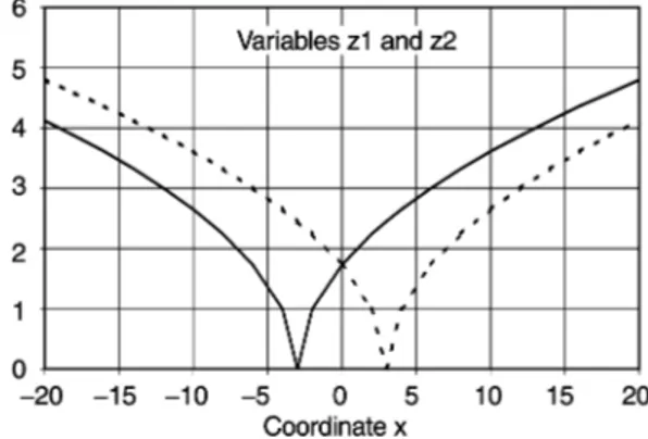
Fig. 6 Variable z1 and z2 used for the Hagaman distance not joined, we de"ne non symmetric membership functions where
the interior spreads are convex and the exterior ones are concave as indicated in Fig. 5; this is done to give more importance to the part of the spreads which are consistent. This method of selecting the membership functions is rather subjective, but the important point is to use the same procedure for all the models.
5. The distance is calculated between the two fuzzy numbers and the operation is repeated for each point of the "rst map.
The method is objective and does not require any special hypothe-ses to be implemented. In particular decisions about size r and related distance are taken on the basis of Monte-Carlo simulations (see Sect. 3.2). The only subjective point is the choice of the member-ship functions which rest on the "nal goal of the analysis (for example, the decision to emphasise matching instead of discrep-ancy), but the consequence is rather limited as long as the same procedure is applied to all the models, the main objective being here to compare these models together.
2.5 A simple application
A simple example is provided here to help to understand the behav-iour of the Hagaman's distance. Consider two variables z1 and z2, de"ned on the dimension x as follows:
z1"Dx#3D0.5
The second variable z2 is obtained by o!setting z1 by 6 units:
z21"Dx!3D0.5
These two variables are de"ned over a domain [!20, 20] and are plotted in Fig. 6. The Euclidian distance between these two curves increases from 0 (for x"0) to a maximum of 6.0 for x"$3 and decreases then towards 0 when x becomes arbitrarily large in abso-lute value. The latter situation corresponds to the case of null domain size in Fig. 7.
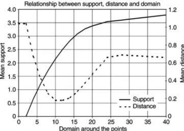
If we de"ne the fuzzy numbers as indicated in Fig. 5, with a pro-gressively larger domain, the support of the fuzzy numbers increase with the size of the domain. The support averaged over all points of the curves is shown in Fig. 7. The mean distance between the curves (calculated for all the points of the curves) has a more complex behaviour: it decreases from a maximum 1.04 to a minimum of 0.18 for domain size between 10 and 12 and increases again to stabilise at about 0.66 from size 24 (this value is linked to the maximum spread of x used here).
Figure 8 represents the dependence of these distances on x. For domain sizes lower than 6, the shape of distance pro"les are similar (roughly M-shaped like the Euclidian distance). For domain sizes between 8 and 20, the distance has a peak for x"0 and decreases towards the extremities and for domain sizes higher than 20, we have spurious secondary peaks at the extremities due to the x interval limited to [!20, 20].
Fig. 7 Evolution of the support and the mean distance in function of the domain size
Fig. 8 Distance between the two variables de"ned in Fig. 6 for several values of the domain size
These pro"les show that for small domains, Hagaman distance has a behaviour similar to the Euclidean distance, but for domains comparable to or larger than the typical scale of the phenomena to be represented, Hagaman distance smooths the e!ects of the pattern shifts smaller than this scale. Domains close to the entire range of the coordinates induce boundary perturbations, so the domain size should be limited to no larger than half the range.
3 The application to model-data comparison
3.1 Data and model simulations
The data used for the comparison are the climatic
reconstructions of Cheddadi et al. (1997) for 6000 y BP
obtained from pollen data constrained by lake-status
indices. The climatic parameters reconstructed are: the
temperature of the coldest month (MTCO), the
grow-ing-degree days above 5 3C (GDD5) and the annual
precipitation minus evapotranspiration (P!E). The
method used for these reconstructions can be
sum-marised as follows: (1) for each 6 ka site, a set of nearest
modern samples (analogues) is determined, (2) the value
of P!E anomaly (i.e. deviation from the modern value
in the 6 ka site) for each analogue is compared with the
status anomaly (i.e. deviation between 6 ka status and
modern status) of the closest lake available and the
analogues which have a P!E anomaly with an
oppo-site sign of the lake status are rejected; (3) the
recon-structed climate is the average of the climate of the
selected analogues; and (4) the error bars of the
recon-structions are given by the variability among the
cli-mate of the di!erent analogues.
Following Masson et al. (1999), we compare model
results with the reconstructed MTCO, GDD5 and
P!E. These parameters can easily be computed from
model output. As permitted by the fuzzy approach, we
do not use the gridded maps presented in Cheddadi
et al. (1997) but rather the reconstructions at the 371
sites (see e.g. in Fig. 9).
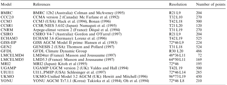
Seventeen climate models (Table 1) involved in the
Paleoclimate
Modelling
Intercomparison
Project
(PMIP) are compared to these data in the region 35 3N
to 90 3N and 10 3W to 60 3E. The models have a wide
range of resolutions and consequently the number of
gridpoints belonging to the region studied ranges
from 72 (for LMD4) to 525 (GEN2 and ECHAM3). All
the simulations of the 6000 BP climate have been
performed with exactly the same prescribed changes
in boundary conditions relative to the present ones.
Orbital parameters have been changed according to
Berger (1978), the atmospheric CO2 content has been
decreased from 345 for modern to 280 for 6000 BP
(Raynaud et al. 1993). Seasonal sea-surface temperature
and sea-ice extent were held to present-day values. Past
Fig. 9 Anomalies of the temperature of the coldest month (6 k - modern) in Europe, as reconstructed from pollen and lake-levels (Cheddadi et al. 1997)
Table 1 Characteristics of the 17 models used for the comparison, including the number of gridpoints belonging to the region studied (35 3N}90 3N, 10 3W}60 3E )
Model References Resolution Number of points
BMRC BMRC 12b2 (Australia): Colman and McAveney (1995) R21 L9 204
CCC2.0 CCMA version 2 (Canada): Mc Farlane et al. (1992) T32 L10 270
CCM3 CCM3 (USA): Hack et al. (1994), Bonan (1996) T42 L18 500
CCSR1 CCSR/NIES 5.4.02 (Japan): Numaguti et al. (1995) T21 L20 120
CNRM Arpege-climat version 2 (France): DeHqueH et al. (1994) T31 L19 270
CSIRO CSIRO V4-7 (Australia): Gordon and O'Farrel (1997) R21 L9 204
ECHAM3 ECHAM 3.6 (Germany): Lorenz et al. (1996) T42 L19 525
GISS-IIP GISS AGCM Model II prime: Hansen et al. (1983) 72*46 L9 224
GEN2 GENESIS 2 (USA): Thomson and Pollard (1997) T31 L18 524
GFDL GFDL Climate Dynamic Group R30 L20 486
LMCELMD4 LMD4ter (France): Masson and Joussaume (1997) 48*36 L11 72
LMCELMD5 LMD5.3 (France): Masson and Joussaume (1997) 64*50 L11 169
MRI2 MRI2 (Japan): Kitoh et al (1995) 72*46 195
UGAMP UGAMP UGCM version 2 (UK): Valdes and Hall (1994) T42L 19 500
UIUI11 UI11}PMIP (USA): Schlesinger et al. (1997) 72*46 L14 285
UKMO UKMO-Uni"ed Model 3.2 AGCM (UK): Hewitt and Mitchell (1996) 96*73 L19 450
YONU YONU AGCM Tr7.1.1 (Korea): Takioka et al. (1984), Oh et al. (1994) 72*46 L8 210
changes in land surface cover have also been neglected,
as requested by PMIP, which can be a major reason for
discrepancies between data and models. As shown by
Texier et al. (1997), the replacement of tundra by boreal
forest in the north of Eurasia contributes to change the
e!ect of surface conditions towards a warming.
Complete maps for all the model simulated changes
in the three bioclimatic parameters can be found in
Masson et al. (1999), as well as a discussion of the
simulated present-day patterns of these parameters.
All the models simulate qualitatively the observed
southwest/northeastern
temperature
gradient
of
modern MTCO. The largest di!erences between model
and observations are found in the northeastern part
of Europe where interannual variability is
impor-tant. They exceed 5 3C only for two simuations.
The north-south gradient of modern GDD5 is also
reproduced by all the models. Over northern Europe,
the departure between models and observations do not
exceed 300 3C days, except for three simulations with
a warm bias (more than 2 3C in average) during the
growing season. The annual water budget
(precipita-tion minus evapora(precipita-tion) is more di$cult to be
simulated because it involves sub-grid scale processes.
Most of the models overestimate the water budget, as
estimated from observation by Masson et al. (1999), up
to a factor 4 to 9 in northeastern Europe. Here, to
illustrate the model behaviour, we only present data
and simulations of MTCO as 90%-level box plots
according to the latitude (Fig. 10). The error bars
ac-count for the dispersion in longitude. This
representa-tion has been chosen because the 6000 BP climate
change reconstructed from pollen exhibits a prominent
north-south gradient (Fig. 9). All the reconstructed
temperatures are negative below 40 3N latitude and
most of them are positive above 50 3N. The models
with the most similar gradient, at least for the southern
part of the map, are ECHAM3, LMD4, YONU,
CCSR1 and GFDL. We present also models with
op-posite gradient (CCC2) or no signi"cant gradient
(BMRC, CCM3). Although there is a large diversity of
the model results, none of these models are really able
to reproduce the magnitude of the changes
reconstruc-ted from the data, especially the negative anomalies of
the south.
3.2 Results
The method developed in Sect. 2 has been applied to
compare each model with data over the whole region.
The exponents p and q are selected as illustrated in
Fig. 5, i.e. the right spread of the smallest number and
the left spread of the greatest number receive exponent
2 and the two other spreads receive exponent 0.2. From
the Hagaman distance computed for each model
grid-point, a mean Hagaman distance is obtained for the
entire map.
This procedure is repeated from various domain
sizes from 13 to 203 (note that low sizes tend toward the
classical Euclidian distance and higher sizes tend to
smooth the variations in the maps), and at each
iter-ation, a mean distance is calculated. Figure 11
illus-trates two examples of the evolution of the distance
according to the domain size for MTCO for two
mod-els: LMD4, with the lowest resolution, and UKMO,
with one of the highest resolutions. The mean distance
MD is represented with its 5%-upper limit MD`,
de-"ned by 2 standard errors around MD (the standard
error being the standard deviation divided by square
root of the number of data points, say 371). To assess
the con"dence interval of these distances, the latter is
compared to a Monte-Carlo simulation, obtained as
follows:
1. We randomly mix the coordinates of the MTCO
within both maps and we calculate the mean
dis-tance between the two maps;
2. We repeat the process 100 times;
3. Over these 100 pseudo-samples so obtained, we
cal-culate the mean distance and its standard error;
4. We consider the mean minus twice the standard
error as a lower random limit (at the 5%-level),
denoted RL!;
5. Any mean distance is signi"cant at the 95%-level
when its MD# is less than RL!.
We can see on Fig. 11 that, for LMD4 and UKMO,
the "rst distance signi"cant at the 95%-level is found
at a domain size of 83. However, the distance evolution
is chaotic for the low-resolution model whereas it is
smoother, with a smaller di!erence between the mean
and the upper-limit for the high-resolution model. For
the latter, the signal is clearer.
Finally we retain, for each model and each climatic
parameter, the lowest signi"cant domain size and the
corresponding mean distance. To facilitate the
com-parison, we standardise the distances by dividing them
by the variance of the spatial distribution of the
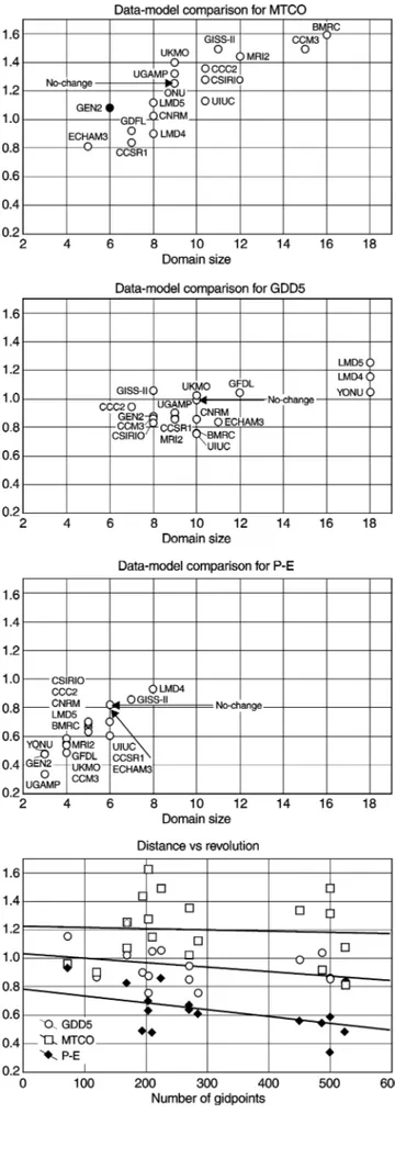
paleodata. They are represented in Fig. 12 as scatter
plots where the ordinate is the distance and the abscissa
is the domain size. This "gure provides a classi"cation
from the closest model to the most distant. All models
with distance below 1.1 produce a warming between 50
and 65 north and a gradient towards colder
temper-ature to the south. Models with the largest distance
exhibits a reverse north/south gradient. An interesting
feature is that the domain size is correlated to the
distance: a close model is already close for low domain
size, even though the resolution also gives a constraint
on this size. Therefore the domain size for the "rst
signi"cant distance comes from a combination of
model resolution (the better the resolution the smaller
the domain size) and of model data-agreement (the
better the agreement the smaller the domain size). For
the two other parameters (Fig. 12), the results are
somewhat di!erent:
A. For GDD5, the models are more consistent with
a distance ranging between 0.7 and 1.1 (three
mod-els have no signi"cant distance and are plotted at
domain size 18: LMD4, LMD5, YONU, which are
among the lowest resolution ones) and, for the
sig-ni"cant models, there is no relationship between the
distance and the domain;
B. For P!E, the distance is lower (between 0.3 and 1)
and, as for MTCO, the domain size tends to
in-crease with the distance.
Considering the relationship between distance and
spatial structure of the simulation, the conclusions are
obvious. For GDD5, data suggest a cooling south of
50 3N and a warming north of 50 3N (Fig. 10). Most of
the models produce a warming over all of Europe, with
the exception of LMD4 and LMD5, for which a
maxi-mum of warming extends towards the Mediterranean.
F ig. 10 B o x p lo ts o f th e d at a o f C he d d a d i et al . (1997) an d si m u lat io n b y ei g h t se le ct ed m o d el s o f th e M T C O p aram et ers , in fu n ct io n o f th e latitu d e. T h e ver ti ca l b a rs re pr es en t the 9 0 th p er cen ti le in te rval a n d the square rep re se n ts th e m ed ian cal cu lat ed o n al l th e g ri d p o in ts in cl u d ed in th e zo n al in terval
Fig. 11 Evolution of the distance between data (Cheddadi et al. 1997) and two simulations of two models (with very di!erent resolu-tions) for the mean temperature of the coldest month (MTCO); the
lines with squares represent the mean distance and mean #2*
standard error calculated on all the gridpoints of the maps between north of 35 3N and 10 3W 603E . The dashed line is calculated by Monte-Carlo simulation and represent the 95% signi"cance level
&&&&&&&&&&&&&&&&&&&&&&&&&&&&&"
Fig. 12 Distance between model simulations and reconstructed data of Cheddadi et al. (1997); three variables are considered: MTCO (the mean temperature of the coldest month), GDD5 (growing-degree days above 5 3C) and P!E (precipitation minus evapotranspira-tion); The "rst three graphs represent "rst signi"cant distance ac-cording to domain size and the last one shows the relationship between distance and the resolution of the models (number of gridpoints in the region considered); the distances are standardized by division by the reconstructed data variance
Thus, they have similar Hagaman distances. For
P!E, the data show more humid conditions over
Europe except in the northwest where dryer conditions
prevail. Several models, like UGAMP, GEN2 and
MRI2, show a similar pattern: their distance is lower
than 0.5 in Fig. 12. Three models (ECHAM3, GISS-II,
LMD4) simulate the opposite pattern. These models
are located above distance 0.8 in Fig. 12.
If we plot the distance versus the resolution of the
model for P!E (Fig. 12d), it appears, that there is
a signi"cant relationship between distance and model
resolution (r
2"0.24): the highest resolution models
all have a distance lower than 0.6. For GDD5, the
relationship is not signi"cant (r
2"0.13) and for
MTCO, the relationship is null (r
2"0.01).
Considering model scores for the three di!erent
cli-matic parameters, we cannot conclude that if a model
&&good'' for one parameter it is necessarily also &&good''
for another one. As an example, ECHAM3 is close for
MTCO, intermediate for GDD5 and distant for P!E.
It is di$cult to understand from these distances
whether a model is really demonstrating something
about the 6 kyr BP climate, or whether in fact any of
these models are better than no model at all. In other
words, is it better to use a climate model to simulate the
6 ka climate than the present-day climatology? To test
this hypothesis, we calculate the distance between the
data and a map of null anomalies, called &&0-change'' in
Fig. 12. It appears that the &&0-change'' is in the middle
of all the models for MTCO and, if we exclude the three
non-signi"cant models for GDD5, there are only two
models poorer than the &&0-change'' for the two other
climatic parameters. Therefore, we conclude that
majority of the models analysed are able to simulate
the 6 ka climate better than they do for the present
climatology.
4 Conclusions
We have applied a new method based on fuzzy logic to
the comparison of PMIP model simulations of the
mid-Holocene with a climatic reconstruction from pollen
and lake-status data over Europe (Cheddadi et al.
1997). This work extends the comparison of Masson
et al. (1999). With the fuzzy logic approach, no
assump-tion is made regarding the distribuassump-tion of the signal and
its error. Also a novelty is that data were taken at the
drilling sites and a varying domain size of comparison
allows us to work at the best common resolution
between observed and simulated maps. In practice, the
larger domain sizes for a given parameter are found
when the model-data agreement is poor. Three
para-meters have been tested: MTCO, GDD5 and P!E.
For each parameter and each model, we compute
a Hagaman distance which gives an objective measure
of the goodness of "t between model and data. The
mean distance for a map is the global score for the
model. On this basis, the di!erent models can be
classi-"ed. It is however possible to have access to a regional
view of the model-data agreement by a map providing
the Hagaman distance at each grid point of the model
grid for the "rst signi"cant domain size at global scale.
The fuzzy logic implies the use of a membership
function of which the shape can be modulated to take
into account some a priori information. Here, this
shape has been chosen to weigh more heavily the part
of the intervals of data and model which overlap, but it
is easily possible to emphasise, for example, where the
part discrepancy is maximum. It is an important
prop-erty of the fuzzy logic to be able to include some a priori
knowledge in the analysis.
Our results show that there is no systematic order for
the three climatic parameters between models. None of
the models satisfactorily reproduce the three
pollen-derived parameters. To evaluate the quality of these
simulations compared to the use of a modern
climatol-ogy in the model-data comparisons, we have also
cal-culated the distance between the data and a map of null
anomalies for the three parameters. Most of the models
are better than this climatology for GDD5 and P!E
and half of them also for MTCO data. There is larger
dispersion in the results for MTCO and P!E than for
GDD5. GDD5 is a integral of temperature and has less
variability than P!E which is generally noisy in
model simulations or than MTCO, which is a winter
time temperature highly variable in middle latitudes.
For the temperature parameters, there is also no
relationship between model resolution and the
Haga-man distance. For instance, results of ECHAM3,
UGAMP and CCM3, the three T42 resolution model
involved in PMIP, cover the whole range of values for
MTCO. But they are rather closer to data for GDD5
than the other models. On the other hand, there is an
inverse relationship between distance and resolution
for P!E (except ECHAM3 which is the only T42
model which poorly simulates that parameter). That
can, perhaps, be explained by the more local character
of P!E which has little chance to be reproduced by
a low-resolution model. Integrated parameters such as
GDD5 have a smoother spatial distribution and show
better consistency between the models. More local
parameters such as P!E need high-resolution models
to be simulated adequately.
As far as data-model comparison is concerned, the
method described here has the advantage when
work-ing on data which have di!erent resolutions and which
are not even gridded. It can help to avoid all form of
bias induced by spatial interpolation. Another
interest-ing point is the fact that the error bars associated with
such maps can be considered. In the absence of
prob-abilistic distributions associated with the Hagaman
distance, a Monte-Carlo method has been used to
assess the signi"cance of this distance.
As this method is based on the distance between
intervals, many other applications involving proximity
analyses can be envisaged. In particular all the methods
based on the research of analogues in the present to
explain past assemblages (or in the recent past to
fore-cast the future) can be improved by such Hagaman
distances. In problems of classi"cation (or cluster
anal-ysis) the errors in the data can be taken into account by
the replacement of the classical Euclidian distance by
the Hagaman distance.
When enough data are available for a larger part of
the globe, it will be possible to provide an overall
evaluation of the models, by averaging the standardised
distances. At this stage, the region is too limited and
does not re#ect the world situation (some regions have
a stronger and more interesting signal, like the East
African monsoon). It is too early for that evaluation
and we want to avoid the impression of a de"nitive
scoring.
Acknowledgements Financial support for this work was provided by the European Union through a grant under the Environment and Climate programme for the project &&Evaluating climate models with proxy-data within the Paleoclimate Modelling Intercomparison Project'' (ENV4-CT95-0075), by the cooperation program between the Commissariat GeHneHral aux Relations Internationales (CGRI) de la CommunauteH franiaise de Belgique, le Fond National de la Recherche Scienti"que (FNRS) and the French Centre National de la Recherche Scienti"que (CNRS). It is a contribution to the Paleo-climate Modelling Intercomparison Project (PMIP).
References
Bardossy A, Bogardi I, Duckstein L (1990) Fuzzy regression in hydrology. Water Resource Res 26 : 1497}1508
Bardossy A, Duckstein, L, Bogardi I (1993) Fuzzy non-linear regres-sion analysis of dose response relationship. Eur J Oper Res 66 : 36}51
Berger A (1978) Long-term variation of caloric solar radiation resulting from the Earth's elements. Quat Res 9 : 139}167 Bonan GB (1996) A land surface model (LSM version 1.0) for
ecological, hydrological, and atmospheric studies, technical de-scription and user's guide. Technical Rep, NCAR Tech Note NCAR/TN-417#STR, Boulder, CO
Braconnot P, Frankignoul C (1993) Testing model simulations of the thermocline depth variability in the tropical Atlantic from 1982 through 1984. J Phys Oceanogr 23 : 626}647
Braconnot P, Frankignoul C (1994) On the ability of the LODYC GCM at simulating the thermocline depth variability in the equatorial Atlantic. Clim Dyn 9 : 221}234
Cheddadi R, Yu G, Guiot J, Harrison SP, Prentice IC (1997) The climate 6000 years ago in Europe. Clim Dyn 13 : 1}9
Colman RA, McAvaney (1995) Sensitivity of the climate response of an atmospheric general circulation model to changes in convec-tive parameterization and horizontal resolution. J Geophys Res 100 (D2) : 3155}3172
DeHqueH M, Dreveton C, Braun A, Cariolle D (1994) The AR-PEGE/IFS atmosphere model: a contribution to the French community climate modelling. Clim Dyn 10 : 249}266
Dong B, Valdes PJ (1995) Sensitivity studies of northern hemisphere glaciation using an atmospheric general circulation model. J Clim 8 : 2471}2496
Dubois D, Prade H (1979) Fuzzy real algebra: some results. Fuzzy Set Syst 2 : 327}348
Duche(ne C, Frankignoul C (1991) Seasonal variations of surface dynamic topography in the tropical Atlantic: observational un-certainties and model testing. J Mar Res 49 : 223}247
Frankignoul C, Duche(ne C, Cane MA (1989) A statistical approach to testing equatorial ocean models with observed data. J Phys Oceanogr 19 : 1191}1207
Frankignoul C, Fevrier S, Sennechael N, Verbeek J, Braconnot P (1995) An intercomparison between four tropical ocean mod-els, thermocline variability. Tellus 47 A : 351}364
Gordon HB, O'Farrell SP (1997) Transient climate change in the CSIRO coupled model with dynamic sea-ice. Mon Weather Rev 125 : 875}907
Hack JJ, Boville BA, Kiehl JT, Rasch PJ, Williamson DL (1994) Climate statistics from the National Center for Atmospheric Research community climate model CCM2. J Geophys Res 99 : 20 785}20 813
Hansen J, Russell G, Rind D, Stone P, Lacis A, Lebede! S, Reudy R, Travis L (1983) E$cient three-dimensional global models for climate studies: models I and II. Mon Weather Rev 111 : 609}662
Harrison SP, Yu G, Tarasov PE (1996) Late Quaternary lake-level record from northern Eurasia. Quat Res 45 : 138}159
Harrison SP, Jolly D, Laarif F, Abe-Ouchi A, Herterich K, Hewitt C, Joussaume S, Kutzbach JE, Mitchell J, De Noblet N, Valdes P (1998) Intercomparison of simulated global vegetation distri-butions in response to 6 kyr BP orbital forcing. J Clim 11 : 2721}2742
Hewitt CD, Mitchell JFB (1996) GCM simulations of the climate of 6 kyr BP: Mean change and interdecadal variability. J Clim 9 : 3515}3529
Jolly D, Prentice IC, Bonne"lle R, Ballouche A, Bengo M, Brenac P, Buchet G, Burney D, Cazet JP, Cheddadi R, Edorh T, Elenga H, Elmoutaki S, Guiot J, Laarif F, Lamb H, Lezine A-M, Maley J, Mbenza M, Peyron O, Reille M, Reynaud-Farrera I, Riollet G, Ritchie J-C, Roche E, Scott L, Semmanda I, Straka H, Umer M, Van Campo E, Vilimumbalo S, Vincens A, Waller M (1998) Biome reconstruction from pollen and plant macrofossil data for Africa and the Arabian peninsula at 0 and 6 ka. J Biogeogr 25 : 1007}1028
Joussaume S, Taylor K (1995) Status of the Paleoclimate Modeling Intercomparison Project (PMIP). In: Gates, WL. (ed), Proc 1st Int AMIP Sci Conf, Monterey, CA, WCRP : 425}430
Kattenberg A, Giorgi F, Grassl H, Meehl GA, Mitchell JFB, Stouf-fer RJ, Tokioka T, Weaver AJ, Wigley TML (1996) Climate models } projections of future climate. Climate change, Houghton et al. (eds), 285}357
Kitoh A, Noda A, Nikaidou Y, Ose T, Takioka T (1995) AMIP simulations of the MRI GCM. Pap Meteorol Geophys 45 : 121}148
Liao X, Street-Perrot A, Mitchell JFB (1994) GCM experiments with di!erent cloud parametrizations: comparisons with paleo-climate reconstructions for 6000 years BP. Paleopaleo-climates 1 : 99}123
Lorenz S, Grieger B, Helbigand P, Herterich K (1996) Investigating the sensitivity of the atmospheric general circulation model ECHAM 3 to paleoclimatic boundary conditions. Geol Rundsch 85 : 513}524
Masson V, Joussaume S (1997) Energetic of 6000 BP atmospheric cirulation in boreal summer, from large-scale to monsoon areas. J Clim 10 : 2888}2903
Masson V, Cheddadi R, Braconnot P, Texier D (1999) Mid-Holo-cene climate in Europe: what can we infer from model-data comparisons? Clim Dyn 15 : 163}182
Mc Farlane NA, Boer GJ, Blanchet J-P, Lazare M (1992) The Canadian Climate Center second-generation general circulation model and its equilibrium climate. J Clim 5 : 1013}1044 Mielke PW, Berry KJ, Brier GW (1981) Application of
multi-re-sponse permutation procedures for examining seasonal changes in monthly mean sea-level pressure patterns. Mon Weather Rev 109 : 120}126
Monserud RA, Leemans R (1992) Comparing global vegetation maps with the Kappa-statistic. Ecol Model 62 : 275}293 Numaguti A, Takahashi M, Nakajima T, Sumi A (1995) Description
of CCSR/NIES AGCM. J Meteor Soc Japan (submitted) Oh J-H, Jung J-H, Kim J-W (1994) Radiative transfer model for
climate studies: 1. Solar radiation parameterizations and valida-tion. J Korea Meteorol Soc 30 : 315}333
Preisendorfer RW, Barnett TP (1983) Numerical model-reality inter-comparison tests using small-sample statistics. J Atmos Sci 40 : 1884}1896
Prentice IC, Guiot J, Huntley B, Jolly D, Cheddadi R (1996) Recon-structing biomes from palaeoecological data: A general method and its application to European pollen data at 0 and 6 ka. Clim Dyn 12 : 185}194
Prentice IC, Cramer W, Harrison SP, Leemans R, Monserud RA, Solomon AM (1992) A global biome model based on plant physiology and dominance, soil properties and climate. J Biogeogr 19 : 117}134
Prentice IC, Harrison SP, Jolly D, Guiot J (1998) The climate and biomes of Europe at 6000 y BP: comparison of model
simula-tions and pollen-based reconstructions. Quat Sci Rev
17 : 659}668
Schlesinger MEN, Andronova G, Entwistle B, Ghanem A, Raman-kutty N, Wang W, Yang F (1997) Modeling and simulation of climate and climate change. In: past and present variability of the solar-terrestrial system: measurements, data analysis and theor-etical models, Proc International School of Physics &&Enrico Fermi'', July 1996, Varena, Italy
Raynaud D, Jouzel J, Barmola JM, Chappelez J, Delmes RJ, Losius C (1993) The ice record of greenhouse gases. Science 259 : 926}934
Texier D, de Noblet N, Harrison SP, Haxeltine A, Jolly D, Jous-saume S, Laarif F, Prentice IC, Tarasov P (1997) Quantifying the role of biosphere-atmosphere feedbacks in climate change: coupled model simulations for 6000 years BP and comparison with palaeodata for northern Eurasia and northern Africa. Clim Dyn 13 : 865}882
Thompson SL, Pollard D (1997) Greenland and Antarctic mass balances for present and doubled CO2 from the GENESIS version-2 global climate model. J Clim 10 : 871}900
Tokioka T, Yamagati K, Yagai I, Kitoh A (1984) A description of the Meteorological Research Institute atmospheric general circula-tion model (MRI-GCM-I). MRI Tech Rep 13, Meteorological Research Institute, Ibaraki-ken, Japan, 249 pp
Valdes PJ, Hall NJ (1994) Mid latitude depressions during the ice age. NATO ASI Volume in long term climatic variations } data and modelling, Duglessy JC (ed), 511}531
Willmott CJ, Ackelson SG, Davis RE, Feddema JJ, Klink KM, Legates DR, O'Donnell J, Rowe CM (1985) J Geophys Res 90 (C5), 8995}9005
Wright HE Jr, Kutzbach JE, Webb III T, Ruddiman WF, Street-Perrott FA, Bartlein PJ (1994) Global climates since the Last Glacial Maximum. University of Minnesota Press, Mineapolis
Zimmermann HJ (1985) Fuzzy set theory and its applications, Mar-tinus Nijho!, Boston
Zwiers F, von Storch H (1989) Multivariate recurrence analysis. J Clim 2 : 1538}1553