Study and design of a small kerosene burner

(1)

© Mathieu Béland, 2019

Study and Design of a Small Kerosene Burner

Mémoire

Mathieu Béland

Maîtrise en génie mécanique - avec mémoire

Maître ès sciences (M. Sc.)

(2)

(3)

iii

Résumé

L’objectif principal de ce travail est de concevoir un petit brûleur au kérosène pour étudier la propriété ignifuge de matériaux composites sous attaque de flamme. Les normes AC20-135 et ISO 2685 décrivent de quelle manière les tests pour démontrer la capacité ignifuge d’un matériau doivent se dérouler. Ces normes sont utilisées pour dresser les requis pour la conception de ce petit brûleur au kérosène. Des gouttelettes liquides de jet-A sont pulvérisées pour alimenter la flamme en carburant tandis que l’air est amené via une conduite annulaire autour de l’injecteur. La combustion génère une flamme non-confinée. L’injecteur sélectionné est un atomiseur à pression avec ligne de retour de la compagnie Delavan. Un swirler en impression 3D de plastique est placé dans le brûleur près de la sortie d’air pour augmenter le mélange entre les gouttelettes de jet-A et l’air. Une analyse de mécanique des fluides numériques (MFN ou CFD en anglais) est présentée pour mieux comprendre l’aérodynamique dans un brûleur et pour concevoir le swirler. Le brûleur est conçu pour permettre de facilement changer le swirler pour tester différents angles d’aubes. Un banc d’essai a été mis en place pour tester l’effet de ces swirlers sur le flux thermique de la flamme. Les effets de la puissance du brûleur, du rapport d’équivalence et de la distance entre le brûleur et la position de la mesure ont été investigués avec des essais expérimentaux. Un swirler de 15 aubes avec un angle d’aube de 25° a été choisi. Parmi toutes les distances axiales testées expérimentalement avec le swriler choisi, il est possible d’atteindre le flux thermique requis de 116 kW/m2_{avec le plus de configurations de flamme} possible lorsque cette distance est de 7.6 cm (3 po.) du brûleur. Il est possible de générer une flamme avec un diamètre inférieur à 6.4 cm (2.5 po.) tout en atteignant le flux thermique requis de 116 kW/m2_. Ceci permet d’effectuer des tests sur des petits échantillons et de réduire les coûts des tests de pré-certification. Pour atteindre cette configuration de flamme, il faut ajuster la puissance du brûleur entre 10 kW et 20 kW avec un rapport d’équivalence entre 0.7 et 0.9.

(4)

iv

Abstract

The main objective of this work is to design a small kerosene burner to study the fireproofing capacity of composite material under flame attack. The standards AC20-135 and ISO-2685 described how the fireproofing tests have to be performed and are used to set the requirements for the design of the small kerosene burner. The burner sprays liquid jet-A droplets and air is flowing around the injector in an annular chamber. The combustion generates an unconfined flame. The fuel injector selected is a Delavan spill-return pressure atomizer. There is a custom 3D printed plastic swirler at the air exit near the combustion area to increase the mixing between air and jet-A droplets. A computational fluid dynamic analysis (CFD) is presented to better understand the aerodynamic of the burner and to design the swirler. The design of the burner allows to easily change the swirler to test different vane angles. An experimental test bench is designed to test the effect of these swirlers on the heat flux under multiple combinations of burner power and equivalence ratio at four axial measurement locations. The experimental investigation allows selecting the final configuration and parameters for the burner. The chosen swirler has 15 vanes that are oriented 25° to the burner axis. The best axial location for the measurements is at 7.6 cm (3 in.). It is possible to generate a flame with a diameter smaller than 6.4 cm (2.5 in.) while reaching the required heat flux of 116 kW/m2_{. This accommodates smaller} coupon sizes and reduces cost for pre-certification testing. To achieve this flame configuration, the burner power should be set between 10 kW to 20 kW with an equivalence ratio between 0.7 and 0.9.

(5)

v

List of Tables

Table 1.1 : Requirements of the kerosene burner to design. ... 5

Table 2.1 : Estimation of the burner power. ... 13

Table 2.2 : Estimation of the burner air mass flow rate. ... 17

Table 2.3 : Range of estimated operating conditions. ... 18

Table 4.1: Reference operating conditions for the Imperial College burner. ... 33

Table 4.2: Injection point properties for the Imperial College Burner. ... 35

Table 4.3: Under-relaxation factor for the Imperial College Burner. ... 37

Table 5.1: Physical characteristics of the main swirlers tested. ... 52

Table 5.2 : Reynolds number associated to the variation of vane angle. ... 53

Table 5.3 : Air velocity angle leaving the swirler calculated with cold flow CFD simulations. ... 55

Table 5.4 : validation of the relation between SMD and FN. ... 59

Table 5.5 : SMD of the selected fuel injector at minimum and maximum fuel pressure. ... 60

Table 5.6 : Summary of the fuel spray parameters. ... 62

Table 7.1 : Surface temperature as function of swirler vane angle. ... 70

Table 7.2 : Tests data of the swirler mapping. ... 72

(8)

viii

List of Figures

Figure 1.1 : Diagram of the heat transfer device presented in Power Pan Engineering Report No. 3A (U.S.

Department of transportation, 1978). ... 2

Figure 1.2 : FAA NexGen Burner (Ochs, 2013). ... 6

Figure 1.3 : Parts of the FAA NexGen burner (Ochs, 2010). ... 6

Figure 1.4 : Stator a) and turbulator b) of the NexGen burner (Federal Aviation Administration, 2016). ... 7

Figure 1.5 : Energy balance of thermocouple (Ochs, Kao, 2013). ... 8

Figure 2.1 : Modified Monarch F-124 turbulator with 4 tabs (Kao, 2012). ... 10

Figure 2.2 : Successful conditions with the NextGen burner. ... 11

Figure 2.3 : Adiabatic temperature rise for jet-A (ΔT) for given Φ for a given air inlet temperature and pressure. ... 14

Figure 2.4 : Iterative process to estimate the error for a measured temperature with a thermocouple. ... 15

Figure 3.1 : Axial swirler. ... 19

Figure 3.2 : Vanes angle of an axial swirler. ... 19

Figure 3.3: Flow recirculation induced by strong swirl. (From Gupta, A.K., Lilley, D.G., and Syred, N., Swirl (Lefebvre, 2010). ... 20

Figure 3.4: Influence of SN on maximum reverse mass flow (Lefebvre, 2010). ... 21

Figure 3.5 : Numerical simulation of airflow around swirler vanes ... 22

Figure 3.6: Variation of the air outlet angle for flat vanes swirler (Kilik, 1976). ... 23

Figure 3.7: Imperial College reference burner (Fossi, 2017). ... 25

Figure 3.8 : Secondary recirculation zone. ... 25

Figure 3.9: 2D Axisymmetric CFD showing the 2 secondary recirculation zones. ... 26

Figure 3.10 : Swirling pipe flow showing the rotation of vorticity (Dennis, 2014). ... 27

Figure 3.11 : Initial conditions of the swirling pipe flow. ... 27

Figure 3.12 : Induce reverse flow by the torus of vorticity. ... 28

Figure 3.13 : Non-viscous rotational vorticity component. ... 29

Figure 4.1: Dimensions of the Imperial College burner (Fossi, 2017). ... 32

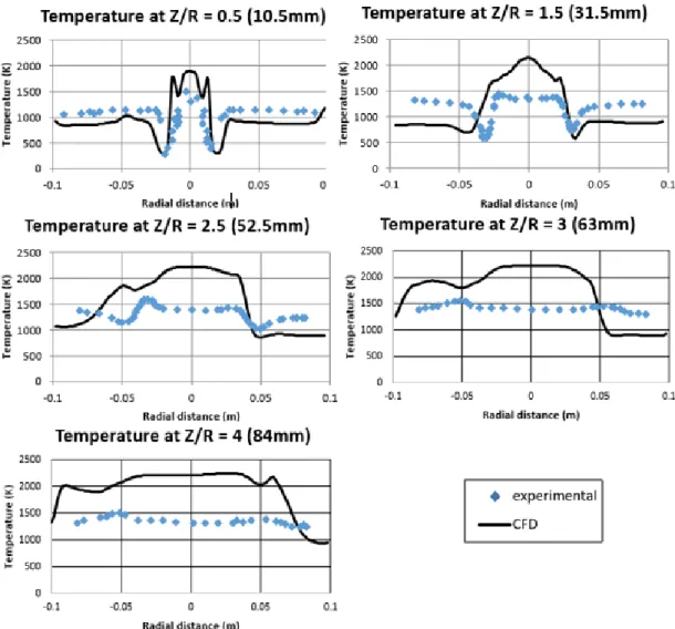
Figure 4.2 : Comparison of the axial velocity predicted with CFD to the experimental data. ... 38

Figure 4.3 : Comparison of the tangential velocity predicted with CFD to the experimental data. ... 39

Figure 4.4 : Comparison of the temperature predicted with CFD to the experimental data. ... 40

Figure 5.1 : Installation schematic of a spill-return fuel injector (Delevan, 2016). ... 42

Figure 5.2 : Drawing of the spill-return injector selected (Delavan, 2016)... 44

Figure 5.3 : Spill-return line in the radial direction. ... 44

Figure 5.4 : Flame with the spill-return line in the radial direction. ... 45

Figure 5.5 : Spill-return fuel injector assembly. ... 45

Figure 5.6: Sectional view of the burner. ... 46

Figure 5.7: Retaining rings. ... 47

Figure 5.8: Outer and inner nozzle. ... 47

Figure 5.9: Fuel adaptor. ... 48

Figure 5.10 : Heat transfer towards the swirler. ... 49

Figure 5.11 : Section view of the swirler. ... 50

Figure 5.12 : Mesh for the swirler with 30° vane angle. ... 54

Figure 5.13 : Vectors colored by velocity magnitude with the swirler with 20° vane angle. ... 55

(9)

ix

Figure 5.18 : SMD as a function of fuel pressure for the three FN (Rizk, 1985). ... 59

Figure 5.19 : Cumulative drop-size distribution (Rizk, 1985). ... 60

Figure 5.20 : Comparison of the Rosin-Rammler to the experimental cumulative drop-size distribution. ... 62

Figure 6.1: Schematic view of the burner and its instruments. ... 64

Figure 6.2: Picture of the burner in operation. ... 64

Figure 6.3: a) Support with the rake of thermocouples. b) Support with the calorimeter in place. ... 65

Figure 6.4 : a) Thermocouple rake during flame temperature measurement, b) position and dimension of the thermocouples. ... 66

Figure 6.5 : a) Custom calorimeter in the flame and b) aligned with the axis of the injector. ... 67

Figure 6.6 : Location of the thermocouple measuring the burner surface temperature. ... 69

Figure 7.1 : Surface temperature with swirler of 38° vane angle. ... 70

Figure 7.2 : Surface temperature with swirler of 30° vane angle. ... 71

Figure 7.3 : Influence of the swirler on the flame shape for a swirler with vane angle of a) 40°, b) 30°, c) 25° and d) 20°. ... 73

Figure 7.4 : Ring of fire produced by a swirler with a 60° vane angle. ... 74

Figure 7.5 : Effect of inlet fuel pressure on the heat flux as a function of axial distance for a power of 14 kW and an Φ of 0.75. ... 76

Figure 7.6 : Effect of swirler vane angle at 15 kW and Φ =0.75. ... 76

Figure 7.7 : Effect of swirler vane angle at 15 kW and Φ =0.8. ... 77

Figure 7.8 : Effect of swirler vane angle at 15 kW and Φ =1. ... 77

Figure 7.9 : Flame diameter as function of Φ at different burner powers. ... 79

Figure 7.10 : Flame shape at a burner power of 22 kW with an Φ of a) 0.9 and b) 1.3. ... 79

Figure 7.11 : Flame length as function of Φ at different burner powers. ... 80

Figure 7.12 : Velocity magnitude inside the swirler as a function of Φ at different burner powers. ... 80

Figure 7.13 : Heat flux as function of burner power at four axial locations with an Φ of 0.75. ... 81

Figure 7.14 : Heat flux as a function of burner power at four axial locations with an Φ of 0.85. ... 82

Figure 7.15 : Calorimeter heat flux as function of burner power at four axial locations with an Φ of 1. ... 83

Figure 7.16 : Heat flux as a function of Φ at four axial locations with a burner power of a) 8.7 kW, b) 12.3 kW, c) 15 kW, d) 18 kW, e) 22 kW, f) 30 kW. ... 84

Figure 7.17 : Heat flux as a function of axial distance at an Φ of a) 0.65, b) 0.75 and c) 0.85... 85

Figure 7.18 : Functional conditions at a) 5.1 cm (2in.), b) 7.6 cm (3in.) and c) 10.2 cm (4in.). ... 86

Figure 7.19 : Functional conditions at 7.6 cm (3 in.) with a flame diameter smaller than 6.4 cm (2.5 in.). ... 87

Figure 7.20 : Axial velocity predicted by CFD as function of the radial position at a measurement locations of 5.1 cm (2in). ... 89

(10)

x

Figure 10.2: Drawing of the fuel adaptor. ... 97

Figure 10.3: Drawing of the fuel connector. ... 98

Figure 10.4: Drawing of the inner nozzle. ... 99

Figure 10.5: Drawing of the inner nozzle. ... 100

Figure 10.6: Drawing of the inner tube. ... 101

Figure 10.7: Drawing of the outer tube. ... 102

Figure 10.8: Drawing of the plenum part. ... 103

Figure 10.9: Accuracy of the Coriolis CMF200 used to measure air mass flow rate. ... 104

(11)

xi

Nomenclature

εTC: Thermocouple emissivity ν: Kinematic viscosity ω: Vorticity

θSW: Swirler blade angle. The smaller angle between the axial direction and the blade direction σ: Stefan-Boltzmann constant

C: Swirler vanes chord

CFD: Computing fluid dynamic Cp: Water thermal capacity DC: Calorimeter diameter DF: Flame diameter

DTC: Diameter of the thermocouple bead FN: Flow number

h: Convection coefficient

kair : Conductivity coefficient of the air

LC: Calorimeter reference length to calculate the reference area for the measurement of heat flux 𝑚̇𝐴: Air mass flow rate

𝑚̇𝑓: Fuel mass flow rate

𝑚̇𝑤: Water mass flow rate

n: Spread parameter for the Rosin-Rammler drop-size distribution Nb: Number of blades

Nu: Nusselt number Pr: Prandtl number

q: Spread parameter calculated by Rizk QBurner: Burner power

Rede: Reynolds number based on the hydraulic diameter ReCI: Reynolds number based on the chord length Rhub: Swirler external hub radius

Rsw: External radius of the annular section of the swirler Tb: Blade thickness

Tg: Gas temperature

Tin: Water temperature at the calorimeter inlet Tout: Water temperature at the calorimeter outlet TSW: Swirler thickness

TTC: Thermocouple temperature S: Space between the swirler vanes SMD: Sauter mean diameter SN: Swirler number

Uθ: Rotational velocity

UR: Radial component of velocity UZ: Axial component of velocity

Vgas: Velocity of the air/gas inside the flame W: Tangential component of velocity

(12)

1

1 Introduction

The research presented in this document is part of a multidisciplinary project where the global goal is to study the mechanical, acoustic and thermal properties of fireproof composite material under flame attack. This composite material is used in the by-pass duct of an aircraft powerplant. The project considers the case where a fire comes from outside the engine nacelle. This means that one side of the fireproof material is exposed to an airstream of different velocities and the other side is exposed to a flame of jet-A while the material needs to withstand mechanical loads for which it was designed. Very few experimental data are available in the literature that cover all those aspects. For this reason, the team decided to design a whole rig that will represent as close as possible this reality. One of the major aspects of this test rig is the burner that is used to generate a jet-A flame to attack the sample. This dissertation will present the design and study of this kerosene (jet-A) burner. Firstly, a literature review is presented in order to better understand the complexity of the problematic and to set the requirements for the kerosene burner to design. Two similar burners are presented as reference for the design of the new small burner. This will allow setting the methodological approach to design and test the small burner.

1.1 Requirements from the regulations

It is desired that the tests performed in this project will be similar to the one specified in the standards that regulate the fireproof materials for aircraft powerplant. The parts of an aircraft powerplant that needed to be fireproof must use materials that are certified as fireproof by a competent authority. The Federal Aviation Administration (FAA) and the International Organization of Standardization (ISO) wrote guidelines to regulate and to define what can be considered as a fireproof material in the specific case of an aircraft powerplant. These standards are the AC20-135 (U.S. Department of transportation, 1990), AC33-17A (U.S. Department of transportation, 2009), Power Plant Engineering Report No. 3A (U.S. Department of transportation, 1978) and the ISO-2685 (International Standard, 1998). Some of the requirements written in these standards need to be considered in the design of the kerosene burner and will be discuss in the following lines. The American standards define fireproof as the capability of a part or component to withstand, as well as or better than steel, a flame with an average temperature of 1093°C (± 66°C) and a heat flux of 117 kW/m2_{± 6 kW/m}2_{for a minimum of 15} minutes, while still achieving its functions intended to be performed when exposed to a fire. The ISO-2685 defines fireproof the same way except that the flame temperature needs to be of 1100 °C ± 80°C and the heat flux of 116 kW/m2_{± 10 kW/m}2_{. Seven thermocouples shall measure the required} temperature within the specified margin. According to the AC20-135, the thermocouples to be used

(13)

2

to measure the flame temperature should be with a bare junction of 1.6 mm (l/16 in.) to 3.2 mm (l/8-in.) metal sheathed, ceramic packed, chromel-alumel (type K), thermocouples with nominal 0.3 mm to 0.6 mm (22 to 30 AWG) size conductors or equivalent. An air aspirated, shielded, thermocouple should not be used. The ISO-2685 specify the same type of thermocouples, but with wire size between 0.6 mm to 1 mm. All the standards suggest to use for the heat transfer device the calorimeter presented in the Power Plant Engineering Report No. 3A (U.S. Department of transportation, 1978) and shown on Figure 1.1.

Figure 1.1 : Diagram of the heat transfer device presented in Power Pan Engineering Report No. 3A (U.S. Department of transportation, 1978).

The calorimeter is a copper tube of 381 mm (15 in.) long with an external diameter of 13 mm (0.5 in.) with water flowing inside. The water is coming from a tank at a constant height of 1.5 m (5 ft.) and a metering valve allow the user to adjust the water flow rate. The water temperature is measured at the inlet and outlet of the test section. This way it is possible to calculate the heat transfer from the flame to the water. To get the heat flux, the heat shall be divided by the reference surface. According to AC20-135, the reference surface is the complete external surface of the copper tube. According to ISO-2685, the length used to compute the heat flux is the length of the copper tube exposed to the flame. The standards also regulate the size of the specimen to test and the size of the flame. According to ISO-2685, the area of the specimen cannot be more than twice the area of the flame at the burner nozzle. According to AC20-135, the size of the panel shall be approximately 254 mm (10 in.) by 254 mm (10 in.) and the required heat flux and temperature shall be maintained on an area of approximately 127 mm ( 5 in.) by 127 mm ( 5 in.). The specimen size should be large enough to prevent flame wraparound of the specimen edge to provide a more accurate simulation of the actual installation. For the ISO-2685, the opposite situation can happen, because the user can use a very

(14)

3

small specimen in comparison with the size of the flame. The two standards used the same procedure to calibrate the burner as describe below.

1. Clean the external surface of the copper tube.

2. Set the water supply temperature between 10°C (50 °F) and 21 °C (70 °F). 3. Set water flow rate to 62.5 g/s (500 lb/hr).

4. Light the burner and allow a 3 minutes warm-up.

5. Adjust the parameters of the burner to get the proper flame temperature measured with the thermocouples.

6. Move the burner in front of the calorimeter by keeping the same axial distance between the burner and the calorimeter as the distance between the burner and thermocouples.

7. Measure the heat flux during 3 minutes.

8. Move the burner in front of the material specimen by keeping again the same axial distance. 9. Expose the front of the specimen to the flame and the back face to air flow corresponding to

normal engine operation and vibrations of 0.4 mm of amplitude for 5 minutes.

10. Expose the front of the specimen to the flame and the back face to air flow corresponding to wind milling conditions and no vibrations for 10 more minutes.

According to U.S. standards, the axial distance between the burner and the specimen (and also between the burner and thermocouple or calorimeter) shall be 101.6 mm (4 in.). For the ISO-2685, this distance is not specified to the user, but needs to be the same in the three conditions. Once the test is completed, the standards also regulate the acceptance criteria. For the ISO-2685, the item shall be capable of withstanding the fire test corresponding to the appropriate requirements and/or to its detailed specification. The AC20-135 and AC33-17A add more criteria as describe below.

1. No flame penetration shall be observed.

2. No exhibition of backside ignition for the required test time.

3. No residual fire. For example, a rapid self-extinguishing flame and no re-ignition after test flame removal is generally acceptable.

The test described in the standards only provides a pass or fail result. The requirements are not exactly the same depending on which standard is considered. The goal of the project is to understand the behavior of the specimen under flame attack. For this reason, other requirements directly related with

(15)

4

the project needed to be added. It will then be possible to set the final requirements for the kerosene burner to design.

1.2 Requirements from the project

The objective is to perform as many fireproof tests as possible with a limited quantity of material to test different sample configurations. For this reason, the size of the sample needs to be minimize. It is planned to use samples of 25 mm (1 in.) or 51 mm (2 in.) wide by approximately 254 mm (10 in.) high. The effective area would be 25 mm or 51 mm wide by 51 mm high in the center of the sample. A flame diameter smaller than 51 mm (2 in.) is targeted. This way, the flame will not attack the sample from its edge which would quickly deteriorate the sample and would not be a realistic representation. This respects the two definitions presented in the standards. To prevent the flame wraparound, extension walls are added on each side of the sample. This allows accepting larger flame diameter. The limit on the maximum flame diameter is set at 76 mm (3 in.). One aspect of the project is to create a numerical tool to predict the behavior of the sample under flame attack. This tool will be compared with experimental data provided by the designed kerosene burner. To facilitate the comparison, it is required to generate a steady flame with as much as possible an uniform heat flux and temperature. The flame shape will need to be a solid cone to reach better uniformity. The inlet parameters of the burner which are mainly the fuel flow rate and the air flow rate need to be adjustable. This will allow testing the behavior of the sample under different flame configurations and to respect the margin for heat flux and flame temperature as specified in the standards. The quantity of unburned jet-A droplets is to be minimized to improve combustion efficiency and to avoid producing excessive soot. In the case of a real fire engulfing an aircraft powerplant, this quantity is unknown and uncontrolled. To study the behavior of the sample under a flame attack and to compare it to numerical predictions, it will be easier with a minimum quantity of unburned droplets. The laboratory where the final tests will be performed has a limited capacity to evacuate the combustion products which limit the nominal power of the burner to around 30 kW. This power QBurner is based on the lower heating value (LHV) and the mass flow rate of jet-A as shown in the equation below. The average jet-A LHV is 43.23 kJ/g (Odgers, 1986).

(16)

5

1.3 Final requirements

By considering the requirements of the standards and the requirements of the project, the requirements of the burner can now be written as shown in Table 1.1. The length of the flame is not critical, but the same axial distance from the burner exit to the specimen under fireproof testing needs to be use for the temperature and heat flux measurements. The axial distance of 101 mm (4 in.) specified in the Power Plant Engineering Report No. 3A (U.S. Department of transportation, 1978) is to fit with a specific burner. Here a new burner is to be designed, so the axial distance of 101 mm may not be suitable. It is desired to perform similar tests to what is already done in the standards. The effect of the axial distance will be investigated from 51 mm (2 in.) to 127 mm (5 in.).

Table 1.1 : Requirements of the kerosene burner to design.

Characteristic target Minimum Maximum

Dimension

Flame shape Rectangular or

circular Flame diameter [mm] 38 76 Flame length [mm] 101 51 127 Performance Temperature [°C] 1 100 1 020 1 180 Heat flux [kW/m2_] ₁₁₆ ₁₀₆ ₁₂₆ Power [kW] 30 Flame uniformity On the effective area of the specimen Unburned jet-A droplets To be minimised

1.4 NextGen Burner investigation

The standards suggest a specific burner to perform the tests, but this oil burner has become commercially unavailable. For this reason, the FAA has developed a Next Generation burner (NexGen burner) based on the original oil burner. The aim of the FAA with this replacement burner is to produce a flame similar to the original Park oil burner with a better repeatability, easier to set up and operate. All the drawings and characteristics of the burner are available to the public (Federal Aviation Administration, 2016). The NexGen Burner is shown on Figure 1.2. The diameter of the draft tube is 101.4 mm (4 in.) and the cone exit has an elliptical shape of approximately 279 mm (11 in.) by 152 mm (6 in.). The parts of this burner are shown on Figure 1.3. A Delavan, 80° solid spray pattern, fuel injector calibrated to provide flow rate of 0.126 L/min (2 GPH) is used. This burner has a nominal

(17)

6

power of 85 kW which is much higher than the limit of 30 kW fixed for the design of the new small kerosene burner. Also, the area of the exit cone leads to a flame too large for the size of the specimen that will be tested. For those two reasons, the NexGen burner cannot be used in the present project. An excellent investigation (Ochs, 2013) of this burner provided helpful information for the design of the small kerosene burner. Ochs took many measurements with a particle image velocimetry (PIV) instrument to better understand the airflow inside and outside the burner.

Figure 1.2 : FAA NexGen Burner (Ochs, 2013).

Figure 1.3 : Parts of the FAA NexGen burner (Ochs, 2010).

Each component was tested independently to understand their effects on the airflow pattern. The fuel pipe shown on the left side of Figure 1.3 alone cause a great asymmetry of the airflow pattern leaving the burner. The stator shown on Figure 1.4 a) generates a hollow flow pattern and a strong recirculation

(18)

7

zone near the burner axis. The swirl number (SN) of the stator is 1.15. The turbulator shown on Figure 1.4 (b) generates a more uniform airflow leaving the burner to balance for the non-uniformities created by the upstream elements. The turbulator also increases the velocity of the airflow, prevent the formation of the recirculation zone downstream the stator and breaks the hollow flow pattern.

Figure 1.4 : Stator a) and turbulator b) of the NexGen burner (Federal Aviation Administration, 2016).

Ochs (Ochs, 2013) also performed tests with a modified stator which is more symmetrical and has a higher diameter to fit the diameter of the tube. The results showed a more uniform velocity and temperature fields and a more repeatable flame. The average measured flame temperature was higher. The newly small kerosene burner should be as symmetrical as possible to generate uniform airflow patterns and temperature. Despite those advantages, the symmetrical stator increased the time that the specimen can withstand the flame. This proves that the measured flame temperature alone is not a sufficient criteria to perform standardized fireproof tests. The symmetric stator provided a lower leaving airflow velocity. This means that the air flow velocity could have a high impact on the fireproof capacity of the material as explained in the following paragraph with the error of thermocouple temperature measurement.

1.5 Error in flame temperature measurement with thermocouple

Y. Kao (Kao, 2012) performed many tests similar to those specified in the standards with the FAA NexGen burner. The results of those tests will be helpful to establish a starting point for the required fuel flow rate and airflow rate for the small kerosene burner to design. For all the tests performed, the error in flame temperature measurement was calculated using the energy balance on the thermocouple as shown on Figure 1.5 and equation (1.2). For a fuel flow rate of 0.142 L/min (2.25 GPH), air flow rate of 31.9 L/s (67.6 SCFM), a type K thermocouple with an exposed bead of 3.2 mm (0.125 in.) measuring a temperature of 1322 K, the difference between the flame temperature and the measured

(19)

8

temperature could be higher than 400 K (Ochs, Kao, 2013). This means that the size of the thermocouple and the velocity of the air surrounding the thermocouple have a huge impact on the measured flame temperature that is subsequently used to evaluate the capacity of the specimen to sustain the flame attack. When the burner is set to the same measured temperature, a decrease in air velocity results in an increase in the estimated flame temperature. For the same measured flame temperature, an increase in thermocouple size results in an increase in the estimated flame temperature. The capacity of a specimen to sustain a flame is driven by the estimated flame temperature rather than by the measured flame temperature.

Figure 1.5 : Energy balance of thermocouple (Ochs, Kao, 2013).

∆𝑇 = 𝑇𝑔− 𝑇𝑇𝐶= 𝜎𝜀𝑇𝐶𝑇𝑇𝐶4 ℎ (1.2) where: 𝑇𝑔 = 𝐺𝑎𝑠 𝑡𝑒𝑚𝑝𝑒𝑟𝑎𝑡𝑢𝑟𝑒 = 𝐸𝑠𝑡𝑖𝑚𝑎𝑡𝑒𝑑 𝑓𝑙𝑎𝑚𝑒 𝑡𝑒𝑚𝑝𝑒𝑟𝑎𝑡𝑢𝑟𝑒 𝑇𝑇𝐶 = 𝑇ℎ𝑒𝑟𝑚𝑜𝑐𝑜𝑢𝑝𝑙𝑒 𝑡𝑒𝑚𝑝𝑒𝑟𝑎𝑡𝑢𝑟𝑒 𝜎 = 𝑆𝑡𝑒𝑓𝑎𝑛 − 𝐵𝑜𝑙𝑡𝑧𝑚𝑎𝑛𝑛 𝑐𝑜𝑛𝑠𝑡𝑎𝑛𝑡 𝜀𝑇𝐶 = 𝐸𝑚𝑖𝑠𝑠𝑖𝑣𝑖𝑡𝑦 𝑜𝑓 𝑡ℎ𝑒 𝑡ℎ𝑒𝑟𝑚𝑜𝑐𝑜𝑢𝑝𝑙𝑒 (0.8) ℎ = 𝐶𝑜𝑛𝑣𝑒𝑐𝑡𝑖𝑜𝑛 𝑐𝑜𝑒𝑓𝑓𝑖𝑐𝑖𝑒𝑛𝑡 =𝑁𝑢 ∗ 𝐾𝑔𝑎𝑠 𝐷𝑇𝐶 𝑁𝑢 = 𝑁𝑢𝑠𝑠𝑒𝑙𝑡 𝑛𝑢𝑚𝑏𝑒𝑟 = 0.42𝑃𝑟0.2+ 0.57𝑅𝑒0.5𝑃𝑟0.33 (𝐵𝑟𝑎𝑑𝑙𝑒𝑦, 1998) 𝐾𝑔𝑎𝑠 = 𝐺𝑎𝑠 𝑐𝑜𝑛𝑑𝑢𝑐𝑡𝑖𝑣𝑖𝑡𝑦 𝐷𝑇𝐶= 𝑇ℎ𝑒𝑟𝑚𝑜𝑐𝑜𝑢𝑝𝑙𝑒 𝑏𝑒𝑎𝑑 𝑑𝑖𝑎𝑚𝑒𝑡𝑒𝑟

(20)

9

1.6 Reference burner for CFD

A similar kerosene burner from Imperial College (Sheen, 1993) is also used to design this small kerosene burner. A cross-section of the burner is shown on Figure 3.7. The diameter of the exit cone is 20 cm and the mass flow rate of jet-A is 0.95 g/s which lead to a power of 41 kW. This burner has been studied by Fossi (Fossi, 2017) to create a computational fluid dynamic (CFD) model. Even if the burner power is slightly over the maximum acceptable power, it is useful to use the Imperial College burner to predict the performance or to better understand the behavior of a kerosene burner by using the CFD work.

1.7 Methodological approach

The plan is to scale the geometry of the Imperial College burner and to use the flame-calorimeter interaction of the NexGen burner to design the new small kerosene burner. In chapter 2, the work done by Kao (Kao, 2012) is used to estimate the required jet-A mass flow rate and the air mass flow rate to reach the required heat flux and flame temperature with the new small kerosene burner. The chapter 3 presents an aerodynamic analysis of the Imperial College burner. A good understanding of the aerodynamic of this burner is required to build the appropriate CFD model presented in chapter 4. This CFD model is based on the work done by Fossi (Fossi, 2017) with the Imperial College burner. Once the CFD model is in place and the air and jet-A mass flow rate are estimated, it is possible to select the fuel injector, to design the burner and the swirler as explained in chapter 5. In order to test this new small kerosene burner, an experimental test bench is designed in chapter 6. It is then possible to measure the performances and to compare them with the initial requirements. The chapter 7 presents the main experimental tests. The burner power, the equivalence ratio, the axial distance between the burner exit and the measurement location and different swirler configurations are investigated. All the experimental tests combine with the CFD simulations will allow to select a swirler that generated a flame which the dimensions reach the requirements set previously. The experimental tests will also allow to select the axial distance between the burner and measurement location that allows to reach the required heat flux with the more flame configurations (equivalence ratio and power) as possible.

(21)

10

2 Estimation of the burner operating conditions

The first step of the design process is to estimate the required mass flow rates of jet-A and air to reach the proper heat flux and flame temperature. This estimation is useful to select the appropriate fuel injector and to size the inlet duct where the air is flowing. As a first approximation, it can be considered that the heat flux is mostly driven by the mass flow rate of kerosene and the flame temperature by the equivalence ratio Φ. The equivalence ratio is defined by the equation below which is a measure of the fuel-air mixture.

𝛷 = 𝑚̇𝑓⁄𝑚̇𝑎

(𝑚̇𝑓⁄𝑚̇𝑎)_{𝑠𝑡𝑜𝑖𝑐ℎ𝑖𝑜𝑚𝑒𝑡𝑟𝑖𝑐}

(2.1)

2.1 Estimation of the mass flow rate of jet-A

The goal of this sub-section is to scale the power of the NextGen burner to the new small burner by keeping the same ratio of power that is transferred to the calorimeter as shown in equation (2.5). To estimate the required mass flow rate of jet-A for the small kerosene burner, the data from the NextGen burner (Kao, 2012) are used. The reference data come from a modified version of the NextGen burner. The modification is that four tabs are added to the turbulator as shown on Figure 2.1. This leads to a more homogeneous mixing of the liquid fuel droplets with the gaseous air which increases flame temperature uniformity.

Figure 2.1 : Modified Monarch F-124 turbulator with 4 tabs (Kao, 2012).

From all the conditions presented in Kao’s thesis (Kao, 2012) the ones who reach the measured flame temperature of 1100°C ± 80°C and the heat flux of 116 kW/m2_{± 10 kW/m}2_{are shown on Figure 2.2.}

(22)

11

An average burner power of 83 kW which represents a mass flow rate of jet-A of 1.92 g/s is considered as a reference value to size the new small kerosene burner. The burner power is calculated with equation (1.1).

Figure 2.2 : Successful conditions with the NextGen burner.

The heat that is transferred to the calorimeter QC is calculated with equation (2.2) by knowing the calorimeter inlet water temperature Tin, calorimeter outlet water temperature Tout, the mass flow rate of water 𝑚̇𝑤 and the water thermal capacity Cp.

𝑄𝑐 = 𝑚̇𝑤𝐶𝑝(𝑇𝑜𝑢𝑡− 𝑇𝑖𝑛) (2.2)

In order to get the heat flux q”, the heat that is transferred to the calorimeter needs to be divided by a reference area as shown in the equation below.

𝑞" = 𝑄𝑐

𝑅𝑒𝑓𝑒𝑟𝑒𝑛𝑐𝑒 𝑎𝑟𝑒𝑎=

𝑄𝑐

𝜋𝐷𝑐𝐿𝑐,𝑒𝑥𝑝𝑜𝑠𝑒𝑑 𝑡𝑜 𝑓𝑙𝑎𝑚𝑒

(2.3)

The heat flux measured with the NextGen burner considers the surface of the calorimeter that is exposed to the flame as a reference area as shown in the equation above. The length of the calorimeter used to calculate the exposed area is the width of the burner cone which is 279 mm (11 in.). With the small kerosene burner, the size of the flame will be much smaller. This mean that the required heat

0.6 0.65 0.7 0.75 0.8 0.85 0.9 0.95 1 70 75 80 85 90 95 100 Φ Burner power (kW)

(23)

12

transfer to the calorimeter should be smaller also. By knowing the diameter of the flame DF, the exposed area of the calorimeter can be calculated. Then, the required heat transfer to the calorimeter to reach the heat flux of 116 kW/m2_{is calculated with the equation below.}

𝑄𝑐,𝑛𝑒𝑤 𝑏𝑢𝑟𝑛𝑒𝑟 = 𝑞"𝜋𝐷𝑐𝐷𝐹= 116 [

𝑘𝑊

𝑚2] 𝜋𝐷𝑐𝐷𝐹

(2.4)

At this stage of the project, the combustion efficiency of the new burner is unknown, because the fuel injector, the mass flow rate of jet-A and the fuel-air mixing are unknown. An assumption can be made that the small kerosene burner will have the same combustion efficiency as the NextGen burner. That way, another assumption is made that the ratio of mass flow rate of jet-A on the heat transfer to the calorimeter is proportional for the two burners as shown with the following equation.

𝑚̇𝑗𝑒𝑡−𝐴,𝑁𝑒𝑥𝑡𝐺𝑒𝑛

𝑄𝑐,𝑁𝑒𝑥𝑡𝐺𝑒𝑛

= 𝑚̇𝑗𝑒𝑡−𝐴,𝑛𝑒𝑤 𝑏𝑢𝑟𝑛𝑒𝑟 𝑄𝑐,𝑛𝑒𝑤 𝑏𝑢𝑟𝑛𝑒𝑟

(2.5)

From equation (2.3), the heat transfer to the calorimeter for the NextGen burner is calculated with the equation below.

𝑄𝑐,𝑁𝑒𝑥𝑡𝐺𝑒𝑛= 𝑞"𝜋𝐷𝑐𝐿𝑐,𝑒𝑥𝑝𝑜𝑠𝑒𝑑 𝑡𝑜 𝑓𝑙𝑎𝑚𝑒= 116 [ 𝑘𝑊

𝑚2] ∗ 𝜋 ∗ 0.0127[𝑚] ∗ 0.279[𝑚] = 1.29 𝑘𝑊

(2.6)

By knowing the reference jet-A mass flow rate of 1.92 g/s of the NextGen burner as explained above, the only remaining unknown in equation (2.5) is the jet-A mass flow rate of the new small kerosene burner. The required mass flow rate of jet-A for the new small burner is computed for flame diameters ranging from 25.4 mm (1 in.) to 76.2 mm (3 in.) which match with the burner requirements presented in Table 1.1. These estimates are shown in Table 2.1.

Considering that the diameter of the new burner flame is really smaller than the NextGen burner and the burner specified in the standards, it is planned to use a calorimeter with a smaller diameter. The calorimeter diameter should follow one of the objectives of the project that is to perform equivalent fireproof tests as the tests specified in the standards. At this stage of the project, the air velocity surrounding the calorimeter of the new small kerosene burner is unknown. Anyways, the standards do not specify air velocity surrounding the calorimeter. So, it is not easy to be in similitude. The

(24)

13

strategy used is to keep the same ratio of flame transverse cross-section area to the frontal surface of the calorimeter exposed to the flame. This ratio is of 10.6 for the NextGen burner and the burner specified in the standards. For a flame diameter of 76 mm (3 in.), the calorimeter diameter of the new small burner should be of 5.6 mm (0.22 in.). Due to supply capabilities, a calorimeter diameter of 6.35 mm (0.25 in.) is selected. This calorimeter diameter may be slightly too large for some flame diameters, but higher deviation from the standards may change too much the Reynolds number around the tube and the convection coefficient also. The required mass flow rate of jet-A for the new small burner is computed for a calorimeter diameter DC of 6.35 mm and also 12.7 mm just for information, even if at this higher diameter the similitude is not respected. These estimates are shown in Table 2.1.

Table 2.1 : Estimation of the burner power.

Characteristic unit Calorimeter diameter mm 6.35 6.35 6.35 6.35 12.7 12.7 12.7 12.7 Heat flux kW/m2 ₁₁₆ ₁₁₆ ₁₁₆ ₁₁₆ ₁₁₆ ₁₁₆ ₁₁₆ ₁₁₆ Flame diameter in 1 2 2.5 3 1 2 2.5 3 Flame diameter mm 25.4 50.8 63.5 76.2 25.4 50.8 63.5 76.2 Exposed area m2 _{0.0005 0.0010 0.0013 0.0015 0.0010 0.0020 0.0025 0.0030} Heat transfer kW 0.06 0.12 0.15 0.18 0.12 0.24 0.29 0.35 Jet-A flow rate g/s 0.09 0.17 0.22 0.26 0.17 0.35 0.44 0.52 Burner power kW 3.8 7.5 9.4 11.3 7.5 15.1 18.8 22.6

2.2 Estimation of the mass flow rate of air

Now that the mass flow rate of jet-A is estimated, it is possible to estimate the required Φ and by the same time the mass flow rate of air for each of the cases of Table 2.1. A relation already exists to link the adiabatic flame temperature with the equivalence ratio Φ as shown on Figure 2.3 for jet-A. This relation assumes complete chemical equilibrium. As explained in chapter one, the measured flame temperature does not really represent the real flame temperature. Depending of the air velocity surrounding the thermocouple bead and its size, the error can be as high as 400°C. The burner needs to be operate at a higher Φ (for lean mixture) that the one found with Figure 2.3 to account for this error, the combustion efficiency and the heat loss to the surrounding air. Once that the proper Φ is found, the air mass flow rate is calculated based on the jet-A mass flow rate. Then, the air velocity

(25)

14

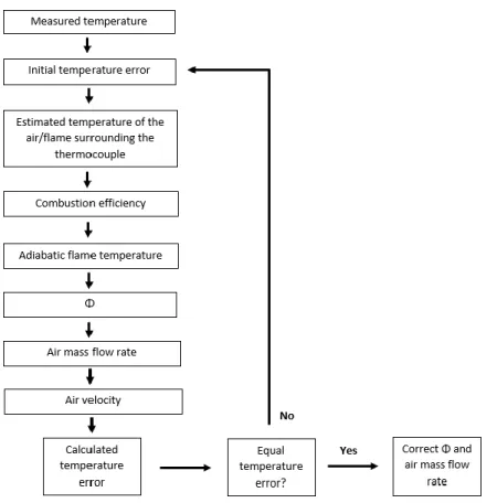
can be estimated to calculate the temperature error. Therefore, an iterative process is taking place as shown on Figure 2.4.

(26)

15

Figure 2.4 : Iterative process to estimate the error for a measured temperature with a thermocouple.

The iterative process starts by setting an initial temperature error that is added to the measured temperature of 1 100 °C which leads to an estimated temperature of the air and/or flame surrounding the thermocouple. To be able to estimate the required Φ by using Figure 2.3, the adiabatic flame temperature ΔTideal of this new burner is missing. By knowing the combustion efficiency, the adiabatic flame temperature is calculated with equation (2.7).

𝜂𝐶𝑜𝑚𝑏𝑢𝑠𝑡𝑖𝑜𝑛=

∆𝑇𝑅𝑒𝑎𝑙

∆𝑇𝐼𝑑𝑒𝑎𝑙

(2.7)

By using equation (2.7), the data of the NextGen burner (Kao, 2012) and the calculated flame temperature surrounding the thermocouple as the real flame temperature, the average combustion efficiency of the NextGen burner is 80%. The same combustion efficiency is used for the design of the new small kerosene burner. The ideal adiabatic temperature is then calculated with equation (2.7). This temperature is used to calculate the required Φ by using Figure 2.3. With equation (2.1), Φ, the mass flow rate of jet-A and by knowing the stoichiometric fuel/air ratio of 0.0668, the mass flow rate

(27)

16

of air is calculated. To estimate the gas velocity Vgas, the density of the combustion products ρgas is used and the area of the flame diameter DF as shown in the equation below.

𝑉𝑔𝑎𝑠 =

𝑚̇𝑔𝑎𝑠

0.25𝜌𝑔𝑎𝑠𝜋𝐷𝐹2

(2.8)

The Reynolds number (Re) is based on the thermocouple bead diameter and the properties of the air at the estimated flame temperature surrounding the thermocouple. The smallest thermocouple allowed by the standards is considered, otherwise the estimated temperature error is too high. The bead diameter is 1.6 mm (0.0625 in.). The Nusselt number (Nu) is then calculated with the equation below.

𝑁𝑢 = 0.42𝑃𝑟0.2+ 0.57𝑅𝑒0.5𝑃𝑟0.33 (𝑏𝑟𝑎𝑑𝑙𝑒𝑦, 1998) (2.9)

The Prandtl number (Pr) is selected at the estimated temperature surrounding the thermocouple. The convection coefficient (h) is calculated with the equation below.

ℎ = 𝑁𝑢 ∗ 𝑘𝑎𝑖𝑟 𝐷𝑇𝐶

(2.10)

The temperature error ΔT is calculated with equation (1.2). The value of the emissivity of the thermocouple bead εTC used here is the same as in chapter one, which is 0.8.

∆𝑇 = 𝑇𝑔− 𝑇𝑇𝐶=

𝜎𝜀𝑇𝐶𝑇𝑇𝐶4

ℎ

(2.11)

This temperature error is compared to the initial temperature error. The initial temperature error is iterated until it is matched with the calculated temperature error. This process is repeated with all the conditions of Table 2.1 and the results are shown in Table 2.2. In some cases, the maximum value of Φ of one is assigned to reach the highest flame temperature, because it is not possible to make the initial temperature error matches with the calculated temperature error. There are some uncertainties related with this procedure to estimate the flame/air temperature surrounding the thermocouple such as the gas velocity, the emissivity of the bead diameter, the correlation for the Nu, etc. To be able to

(28)

17

cover a wider range of air mass flow rate in case that the method related with the temperature error to estimate Φ is not perfectly good, a line in Table 2.2 is added for the calculation of the air mass flow rate without temperature error. In that case, a value of Φ of 0.58 is obtained directly with Figure 2.3 for an adiabatic flame temperature of 1100°C.

Table 2.2 : Estimation of the burner air mass flow rate.

Characteristic unit

Calorimeter

diameter mm 6.35 6.35 6.35 6.35 12.7 12.7 12.7 12.7

Flame diameter mm 25.4 50.8 63.5 76.2 25.4 50.8 63.5 76.2

Jet-A flow rate g/s 0.09 0.17 0.22 0.26 0.17 0.35 0.44 0.52

Burner power kW 3.77 7.54 9.42 11.31 7.54 15.08 18.85 22.62 Initial temperature error K 450 500 500 500 300 450 500 500 Estimated air/gas temperature surrounding the thermocouple K 1823 1873 1873 1873 1673 1823 1873 1873 Adiabatic flame temperature K 2204 2266 2266 2266 2016 2204 2266 2266 Φ 0.91 1.00 1.00 1.00 0.78 0.91 1.00 1.00

Air flow rate with

temperature error g/s 1.43 2.61 3.26 3.92 3.37 5.74 6.53 7.83

Air flow rate without temperature error g/s 2.27 4.54 5.68 6.81 4.54 9.08 11.35 13.62 Gas velocity m/s 15.6 7.3 5.9 4.9 33.4 15.6 11.8 9.8 Re 76 32 26 22 179 76 52 43 Pr 0.683 0.677 0.677 0.677 0.685 0.683 0.677 0.677 Nu 4.77 3.24 2.94 2.72 7.13 4.77 4.00 3.69 h W/(m2_K) ₃₅₈ ₂₆₀ ₂₃₅ ₂₁₈ ₅₀₃ ₃₅₈ ₃₂₀ ₂₉₅ Calculated temperature error K 451 621 685 741 320 451 504 547

(29)

18

2.3 Conclusion of the estimation of the burner operating conditions

The minimum and maximum values of the main parameters in Table 2.2 are put together in Table 2.3 to show the range of operating conditions that are expected for the small kerosene burner. One interesting thing is that the maximum estimated burner power is under the limit of 30 kW imposed by the limitations of the test enclosure. The burner power estimations present some uncertainties, but it will be validated experimentally. On the other hand, it will be more difficult to evaluate properly the flame temperature, due to the difficulty to measure the air velocity surrounding the thermocouple during combustion. The air velocity shown in Table 2.3 is mostly based on the area of the flame diameter and the mass flow rate of air. It does not consider the entrained air from the surrounding air and the axial distance between the burner exit and the location of the temperature measurement. For those reasons, an aerodynamic analysis and a Computational Fluid Dynamic (CFD) approach are presented in the following chapters to better estimate the velocity at the location of the thermocouples.

Table 2.3 : Range of estimated operating conditions. Characteristic unit minimum maximum

Flame diameter mm 25.4 76.2 Jet-A flow rate g/s 0.09 0.52 Burner power kW 3.7 22.6 Φ 0.58 1

Air flow rate g/s 1.4 13.6

(30)

19

3 Aerodynamic analysis

In order to achieve good combustion efficiency, the kerosene droplets and the air need to be well mixed. For this reason, the airflow pattern is of great interest. It also controls the shape, the length and the position of the flame. Different means can be used to reach the desire airflow pattern. Here a swirling flow generated by a swirler will be considered to provide the appropriate air fuel mixing. It is chosen because it can generate predictable airflow pattern. Also, the Imperial College burner studied in Fossi’s thesis (Fossi, 2017) is configured with a swirler. In the perspective to scale the Imperial College burner for the design of the new small kerosene burner, it is easier to have a similar configuration.

3.1 Swirler

An axial swirler is like a turbine stator where air passes through an annular section as shown on Figure 3.1 and Figure 3.2. They are extensively used in gas turbine combustors. They are located at the inlet of the combustion section and concentric to the fuel injector.

Figure 3.1 : Axial swirler.

(31)

20

The blades give a tangential component to the airflow which generates a solid body rotation and induces a recirculation zone that keep the flame close to the injector. This contributes to increase the combustion efficiency, because the vortices in the recirculation zone capture the droplets and return them in the middle of the combustion area to complete their evaporation and combustion. Also, the products of combustion at high temperature are moving upstream which allows the fresh mixture of air-fuel to be ignited and help flame stability. The rotating and recirculating flows are both illustrated in the figure below.

Figure 3.3: Flow recirculation induced by strong swirl. (From Gupta, A.K., Lilley, D.G., and Syred, N., Swirl (Lefebvre, 2010).

To compare the effect of swirler size, blade number, vane chord and angle, the Swirl Number (SN) terminology for constant vane angle is used as defined below by Beer and Chigier (Beer, 1972):

𝑆𝑁 = ∫ 𝑟 2_{𝑊𝑈 𝑑𝑟} 𝑅_𝑠𝑤 0 𝑅𝑠𝑤∫ 𝑟𝑈2𝑑𝑟 𝑅𝑠𝑤 0 (3.1)

(32)

21 𝑆𝑁 = 2 3∗ 1 𝑅𝑠𝑤 ∗ 𝑊 𝑈 ∗ 𝑅𝑠𝑤3− 𝑅ℎ𝑢𝑏3 𝑅𝑠𝑤2− 𝑅ℎ𝑢𝑏2 = 2 3∗ 1 − (𝑅ℎ𝑢𝑏3 𝑅𝑠𝑤3 ) 1 − (𝑅ℎ𝑢𝑏 2 𝑅𝑠𝑤2 ) ∗𝑊 𝑈𝑍 (3.2) where: 𝑅𝑠𝑤= 𝑆𝑤𝑖𝑟𝑙𝑒𝑟 𝑒𝑥𝑡𝑒𝑟𝑛𝑎𝑙 𝑟𝑎𝑑𝑖𝑢𝑠 𝑅ℎ𝑢𝑏= 𝑆𝑤𝑖𝑟𝑙𝑒𝑟 ℎ𝑢𝑏 𝑟𝑎𝑑𝑖𝑢𝑠 𝑊 = 𝑎𝑖𝑟 𝑡𝑎𝑛𝑔𝑒𝑛𝑡𝑖𝑎𝑙 𝑐𝑜𝑚𝑝𝑜𝑛𝑒𝑛𝑡 𝑜𝑓 𝑣𝑒𝑙𝑜𝑐𝑖𝑡𝑦 𝑈𝑍 = 𝑎𝑖𝑟 𝑎𝑥𝑖𝑎𝑙 𝑐𝑜𝑚𝑝𝑜𝑛𝑒𝑛𝑡 𝑜𝑓 𝑣𝑒𝑙𝑜𝑐𝑖𝑡𝑦

According to the work performed by Kilik (Kilik, 1976), when the SN becomes high enough and reaches a critical values of at least 0.4, a recirculation area is formed. The effect of SN on the strength of the recirculation zone is shown on Figure 3.4 by measuring the reverse air mass flow rate. From the literature, a strong swirl is obtained when the SN is of 0.6 or more. From the figure below, a SN of 0.6 is the minimum value to induce reverse flow using flat vanes.

Figure 3.4: Influence of SN on maximum reverse mass flow (Lefebvre, 2010).

The parameter of interest is the angle between the axial and tangential velocity components of the airflow at the exit of the swirler. This angle is shown in equation (3.2 as the velocity ratio W/U and therefore the equation can be re-written below.

(33)

22 𝑆𝑁 = 2 3∗ 1 − (𝑅ℎ𝑢𝑏3 𝑅𝑠𝑤3 ) 1 − (𝑅ℎ𝑢𝑏 2 𝑅𝑠𝑤2 ) ∗ tan 𝜃𝑎𝑖𝑟 (3.3)

In some cases, this angle is the same as the swirler blade angle. From a design point of view, it becomes easier to control the swirl number by varying the blade angle than acting on the hub and swirler diameters who are mainly constrained by the injector geometry. The goal will be to select the appropriate number of blades and blade chord to make sure that the air will follow the blade and leave with the same angle. Achieving this will make the estimation of the swirl number much easier and allow a better prediction of the flow pattern in the combustion chamber.

3.1.1 Swirler blade

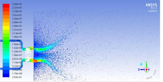
To better understand why the exit air angle could be different from the geometrical blade angle, CFD simulations were performed with ANSYSTM_{Fluent. Flat vanes in an annular section were considered.} Figure 3.5 shows the vector colored by velocity magnitude (m/s) for an airflow coming from the right to the left.

Figure 3.5 : Numerical simulation of airflow around swirler vanes

For a high vane angle, the air near arrow A is not able to follow the vane and the boundary layer separates from the vane. This forms a large separation zone and increases the size of the effective body. The air at the neighbouring vanes (arrow B) is then unable to follow the blade shape due to the separation zone and the surrounding air near arrow A whom has a greater axial component. The

(34)

23

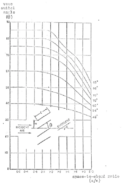
resulting airflow at arrow C has a much smaller angle compared to the geometrical vane angle. This can be solved by reducing the distance between the two blades. So, the air at arrow B will blow on the blade A to force the boundary layer to remain attached.

The experimental studies performed by Kilik (Kilik, 1976) on multiple swirler geometries is of great assistance to predict the air exit velocity angle based on the space-to-chord ratio (S/C) as defined on Figure 3.6. The empirical relation between the geometric and flow angle for different space-to-chord ratios is also illustrated. According to this graph, a maximum space-to-chord ratio of 0.5 is suitable to make sure that the air leaving the vanes will follow it for angles of 40° or more.

(35)

24

Those results were completed at Reynolds number (Rede) of 3x104 to 4x104 based on the hydraulic diameter of the annular section of the swirler. This condition corresponds to a turbulent flow since the Reynolds number is over 4x103_{, which is the typical criteria for internal flow. The Reynolds} number based on the chord (Reci) was around 2x104 to 3.8x104, which is a laminar flow on the blade, because it is below the typical criteria of 5x105_{for flat plate flow. These two Reynolds numbers are} defined as shown below.

𝑅𝑒𝑑𝑒= 2𝑈𝑍(𝑅𝑠𝑤− 𝑅ℎ𝑢𝑏) 𝜈 (3.4) 𝑅𝑒𝑐𝑖 = 𝑈𝑍 𝐶 𝜈 (3.5)

3.2 Mathematical analysis of the recirculating flow

Literatures related to gas turbine combustion and swirler clearly show that an increase in SN increase the size of the recirculation zone. Further analysis of the flow are needed to better select the appropriate SN for a specific situation. For this reason, a mathematical analysis of the flow was performed to understand how the recirculation zone is formed from a rotating flow in an annular section.

3.2.1 Reference burner

The burner used at Imperial College London (Sheen, 1993) and studied with improved interaction between turbulence combustion models in Fossi’s thesis (Fossi, 2017) is used here as an example to illustrate the flow pattern. The geometry of the burner is shown on Figure 3.7. The Reynolds number in the annular section upstream the combustion chamber is 2 x 104_{and the swirl number is 0.9.} /

(36)

25

Figure 3.7: Imperial College reference burner (Fossi, 2017).

3.2.2 Basic recirculation

By considering only the axial velocity component of the air leaving the annular section, the axial velocity distribution shown on Figure 3.8 can be expected. The change in axial velocity induce the two secondary recirculation zones (SRZ) that are also shown on Figure 3.7.

Figure 3.8 : Secondary recirculation zone.

Based on the CFD studies performed by A. Fossi, a 2D axisymmetric simulation of the flow was performed. The velocity vectors colored by the axial component are shown on Figure 3.9. As expected above, the two secondary recirculation zones appear at the same place and are marked by red stars.

(37)

26

Figure 3.9: 2D Axisymmetric CFD showing the 2 secondary recirculation zones.

The third recirculation zone, marked by a green star is the one of interest and briefly described in section 3.1. It is of main importance to control the flame and it will be further explained in the next sub-section.

3.2.3 Primary recirculation zone

The primary recirculation zone is a rotation of the vorticity upstream the section change. A video1_of an experiment (Dennis, 2014) produced by theFluids Engineering Research Group at the University of Liverpool (FERGUL) clearly shows the formation of this type of recirculation zone. Two tubes are connected together where the fluid flows from left to right and a blue marker is added. The left tube is put in rotation and the right one is kept fixed. The rotational speed of the left tube increases with time. After some time, the blue marker starts to accumulate just at the beginning of the second tube which means that a reverse flow start to appear. While the rotational speed continues to increase, a torus of vorticity starts to take place. Just before the end, the reverse velocity is so fast that the blue marker flows upstream of the rotating tube. A picture of the experiment is shown on Figure 3.10.

1_{FERGUL (2014). Vortex Breakdown. [Online video]. Spotted at :}

(38)

27

Figure 3.10 : Swirling pipe flow showing the rotation of vorticity (Dennis, 2014).

The inlet boundary conditions are known as follows: positive axial velocity (UZ>0), positive rotating velocity (Uθ>0) and no radial velocity (UR>0) as shown on Figure 3.11.

Figure 3.11 : Initial conditions of the swirling pipe flow.

From the equation of vorticity below, only the axial component exist at the inlet boundary condition.

With Uθ > 0, a positive axial vorticity is obtained (ωZ > 0).

The decrease of rotational velocity in the second pipe above is represented by the section change from the annular section at the exit of the swirler to the much larger combustion chamber of the burner. In the burner, the air in the annular section downstream the swirler is turning fast at a small diameter. When it comes into the larger section of the combustion chamber, the diameter of rotation of the air

𝜔 = ∇ 𝑥 𝒖 (3.6) 𝜔𝑍 = 1 𝑟 𝑑 𝑑𝑟(𝑟𝑈𝜃) − 1 𝑟 𝑑𝑈𝑟 𝑑𝜃 (3.7)

(39)

28

is greater as it is forced to expand in the larger volume. By conservation of angular momentum, the rotational velocity decreases for a larger diameter. Mathematically this implies that the rotational velocity will be forced to decrease as it progresses in the axial direction:

Now, to explain the formation of the torus of vorticity coming from rotation of vorticity shown in the video, the non-viscous equation of vorticity must be non-zero for the rotational component as expended from equation (3.9) to (3.10).

With a positive axial vorticity and negative variation of the rotational velocity according to the axial displacement as shown in equations (3.7) and (3.8) the overall equation (3.10) is negative. By keeping the same plane of representation as shown in Figure 3.11, the torus of vorticity can be visualized with a cut along the central plane as two vortices inducing reverse flow in the middle of the pipe as represented in Figure 3.12.

Figure 3.12 : Induce reverse flow by the torus of vorticity.

To validate that the airflow behaviour of the two pipes experiment can be compared to the airflow pattern of the Imperial College burner, which implies that the recirculation shown by a green star on Figure 3.9 is rotational vorticity, a CFD simulation was performed. On Figure 3.13, the same

𝑑𝑈𝜃 𝑑𝑧 < 0 (3.8) 𝑑𝜔 𝑑𝑡 = 𝝎 ∙ ∇𝒖 (3.9) 𝑑𝜔𝜃 𝑑𝑡 = 𝜔𝑟 𝑑𝑈𝜃 𝑑𝑟 + 𝜔𝜃 𝑟 𝑑𝑈𝜃 𝑑𝜃 + 𝜔𝑧 𝑑𝑈𝜃 𝑑𝑧 + 𝑈𝑟𝜔𝜃 𝑟 ≠ 0 (3.10)

(40)

29

simulation as the one shown in Figure 3.9 is used. The rotational vorticity (ωθ) is shown and at the position of the green star there is a negative vorticity. So, the mathematical approach matches with the CFD result and allows to better understand this behaviour of the airflow in the combustion chamber.

Figure 3.13 : Non-viscous rotational vorticity component.

3.3 Aerodynamic conclusion

This shows that it is not only the swirl number that affects the size of the recirculation, but also the magnitude of the section change. This leads to a trade-off for the section change. For the same swirl number, a fast variation of the flow area as shown in the previous page conducts to a strong recirculation zone, but at the same time creates two secondary recirculation zones. These zones can be unfavorable, because they can capture the droplets and prevent them to participate in the combustion. This situation reduces the efficiency of the burner. Also, these non-participating droplets will generate soot on the burner walls with a local too rich fuel to air mixture. It is also possible to select a fuel injector with a narrow spray angle and this way the droplets will not go in the secondary recirculation zones. On the other hand, a slow variation of the flow area will generate smaller secondary recirculation, but also a weaker primary recirculation zone and decrease the level of mixing between air and droplets which will reduce combustion efficiency. Depending of the requirement of

(41)

30

the burner, the geometry of the section change and the swirler must be both taken into consideration in the design of the burner.

In this project, there is a requirement to minimize the diameter of the flame. A high primary recirculation zone will force the air to flow around the center and then increase the diameter of the flame. On the other hand, a small recirculation zone will probably make a smaller flame diameter, but will reduce the efficiency. This way, the power of the burner and likely the equivalence ratio will need to be increased to reach the require flame temperature and power. There is also a requirement to reach the flame temperature and power with the smallest burner power. During the design and testing processes, it will be important to try to optimize the size of the recirculation zone by keeping those aspects in mind.

(42)

31

4 CFD model

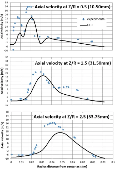
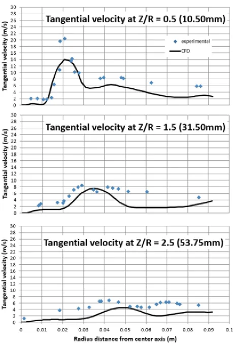
Knowing the behavior of the airflow in the burner as explained in the previous chapter, a proper CFD model can now be chosen to simulate the burner in operation. A CFD model will be useful to design the shape of the burner and to estimate the burner operating conditions (air mass flow rate, kerosene mass flow rate). The goal of this section is to establish all the required parameters in ANSYS FluentTM to reach a realistic simulation. The result will be validated with the experimental data provided in Fossi’s thesis (Fossi, 2017) for the Imperial College burner. Once this will be achieved, it is reasonable to think that by slightly changing the geometry and operating conditions to the requirements of the small kerosene burner, the performances predictions should be fairly realistic also.

The parameters are chosen according to Fossi’s thesis (Fossi, 2017) and ANSYS FluentTM_{user guide} (Ansys, 2013). One major difference is to perform steady state simulations rather than unsteady simulations. The longer calculating time for the unsteady simulation is the reason why it is desire to reach acceptable results with steady simulation from a design point of view. It will be necessary to perform many simulations with different geometries and operating conditions in order to reach the final design. The goal will be to observe the effects of those changes rather that the absolute result. At the end, it will be possible to tune the real burner during operation to reach the desire result.

4.1 Geometry and meshing

The dimensions of the CFD model for the Imperial College burner are shown on Figure 4.1. The swirler vanes are not taken into consideration for the simulation. Axial and tangential velocity components will be use instead to represent the air leaving the swirler.

(43)

32

Figure 4.1: Dimensions of the Imperial College burner (Fossi, 2017).

A hexahedral 3D mesh of 1.2 million nodes is used. The elements are spread similarly as the mesh shown in Fossi’s thesis, with a higher density near the central axis.

4.2 Cold flow simulation

To facilitate convergence and to reduce the calculation time for a steady combustion simulation, it is suggested to start by simulating only the cold flow until convergence is obtained. These simulations are done without droplets injections and without combustion. The pressure based solver is used.

4.2.1 Turbulence model

For flow with high recirculation and SN higher than 0.5, it is strongly recommended to use a more sophisticated turbulence model such as the Reynolds Stress Model (RSM). There are four sub-models within the RSM options offered to take into consideration the pressure-strain term as explained in the ANSYS FluentTM_{theory guide section 4.9.4 (Ansys, 2013). The Stress-Omega model is selected as} the better option. This model is ideal for modeling flow over curved surfaces and swirling flow at low Reynolds. No wall treatment needs to be selected with this pressure-strain model. The option for low-Re correction is selected because the low-Re of the air in the annular section is around 2.4x104_{. The shear} flow correction is kept active.

4.2.2 Boundary conditions

The operating conditions are shown in Table 4.1. A velocity inlet is chosen for the inlet boundary condition. An absolute reference frame is used with an initial gauge pressure of zero Pa. For the turbulence, an intensity of 10 % is selected, because of the presence of the swirler upstream (Fluent